Abstract
Nonlinear distortion has always been a challenge for optical communication due to the nonlinear transfer characteristics of the fiber itself. The next frontier for optical communication is a second type of nonlinearities, which results from optical and electrical components. They become the dominant nonlinearity for shorter reaches. The highest data rates cannot be achieved without effective compensation. A classical countermeasure is receiver-side equalization of nonlinear impairments and memory effects using Volterra series. However, such Volterra equalizers are architecturally complex and their parametrization can be numerical unstable. This contribution proposes an alternative nonlinear equalizer architecture based on machine learning. Its performance is evaluated experimentally on coherent 88 Gbaud dual polarization 16QAM 600 Gb/s back-to-back measurements. The proposed equalizers outperform Volterra and memory polynomial Volterra equalizers up to 6th orders at a target bit-error rate (BER) of by 0.5 dB and 0.8 dB in optical signal-to-noise ratio (OSNR), respectively.
1. Introduction
Modern communication networks build upon a backbone of optical systems, which have fiber as the transmission medium. Due to its physical properties, including the Kerr effect, fiber communication is always affected by nonlinearities. This is the obvious, but not the only major source of nonlinear distortion in optical communication systems. Regardless of the individual technology choices for the optical transceiver architecture, it will always comprise a large number of optical/electrical (O/E) components with nonlinear transfer characteristics, often with memory effects. Their limitations on the achievable capacity are aggravated by measures towards higher data rates, such as symbol rate increase or the shift to higher order pulse amplitude modulations (PAM) and quadrature amplitude modulations (QAM). Nonlinear compensation for O/E components is not yet a standard feature in today’s optical transceivers, but will inevitably become a key element of digital signal processing (DSP) to keep up with ever increasing data rates. Especially when high-bandwidth (BW) communication meets short reach, reduced fiber lengths turn components into the dominant source of nonlinearities. Typical use cases include data center interconnect (DCI) with a range of 80–120 km [1]. Volterra nonlinear equalizers (VNLE) have proven very effective against both, fiber nonlinearities [2] and component nonlinearities [3,4]. They approximate with analytical models based on Volterra series, which can be tailored to match any nonlinear system by choosing a high enough polynomial order P and memory depth M [5] and a set of coefficients (kernels), one for each order/memory tap combination. Excessive scalability, however, can become a crucial downside, as the architectural complexity of VNLEs increases exponentially with P and M. A popular reduced-size alternative are memory polynomial (MP) VNLEs, which operate only on a subset of kernels [6]. However, this reduction costs effectiveness.
Another critical disadvantage of both VNLEs and MP-VNLEs is numerical instability when identifying and extracting the VNLE kernels with the preferred approach, a least squares (LS) solver. This limits in practice the maximum polynomial order P and memory depth M. These shortcomings make general VNLEs and MP-VNLEs far from ideal, which motivate to assess an alternative equalizer structure based on deep neural networks (DNN) in this article. The performance of VNLEs and MP-VNLEs is benchmarked against DNN nonlinear equalizers (NLE) on basis of coherent dual polarization (DP) 16QAM back-to-back (BtB) offline captures, which are reprocessed for all options. For the measurements, a DCI compatible net bit rate of 600 Gb/s with 15% FEC overhead has been chosen. We like to highlight that the universal and flexible nature of both Volterra-based equalizers and DNN equalizers is not limited to this exemplary configuration. One can expect benefits for different reaches, data rates or even detection technologies, such as IM-DD with PAM modulation. We focus on coherent systems here, since we target a single lambda system for our 600 Gb/s data rate. This is out of scope for IM-DD, due to its limited spectral efficiency.
2. Principles of Nonlinear Equalizer
The presented BtB setup focuses on component nonlinearities, while the compensation of fiber nonlinearities has been shown before [7]. For this paper, DNN structures have been implemented from scratch with Matlab, not using any machine learning (ML) toolbox. Being trained on the same data as (MP-)VNLEs, DNNs learn to capture nonlinear effects of O/E components and fiber, as well as their memory characteristics.
2.1. General Volterra Equalizer
With and representing system input and output, respectively, the Pth-order discrete time Volterra series with memory taps for order p is given as [8]
It is the most complete model for nonlinearities with memory, as the pth-order Volterra kernel includes all possible combinations of a product of p time shifts of the input signal up to memory depth .
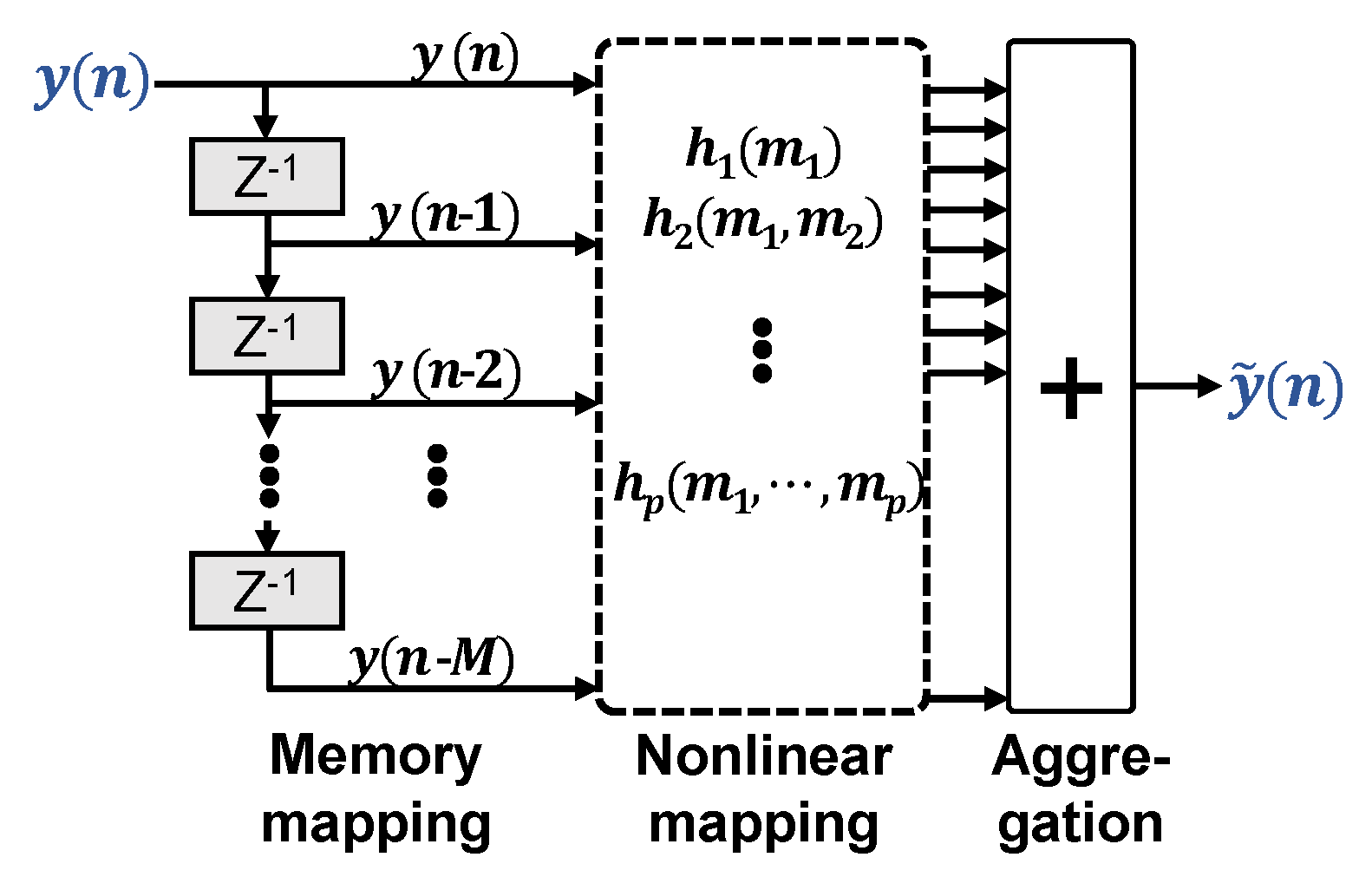
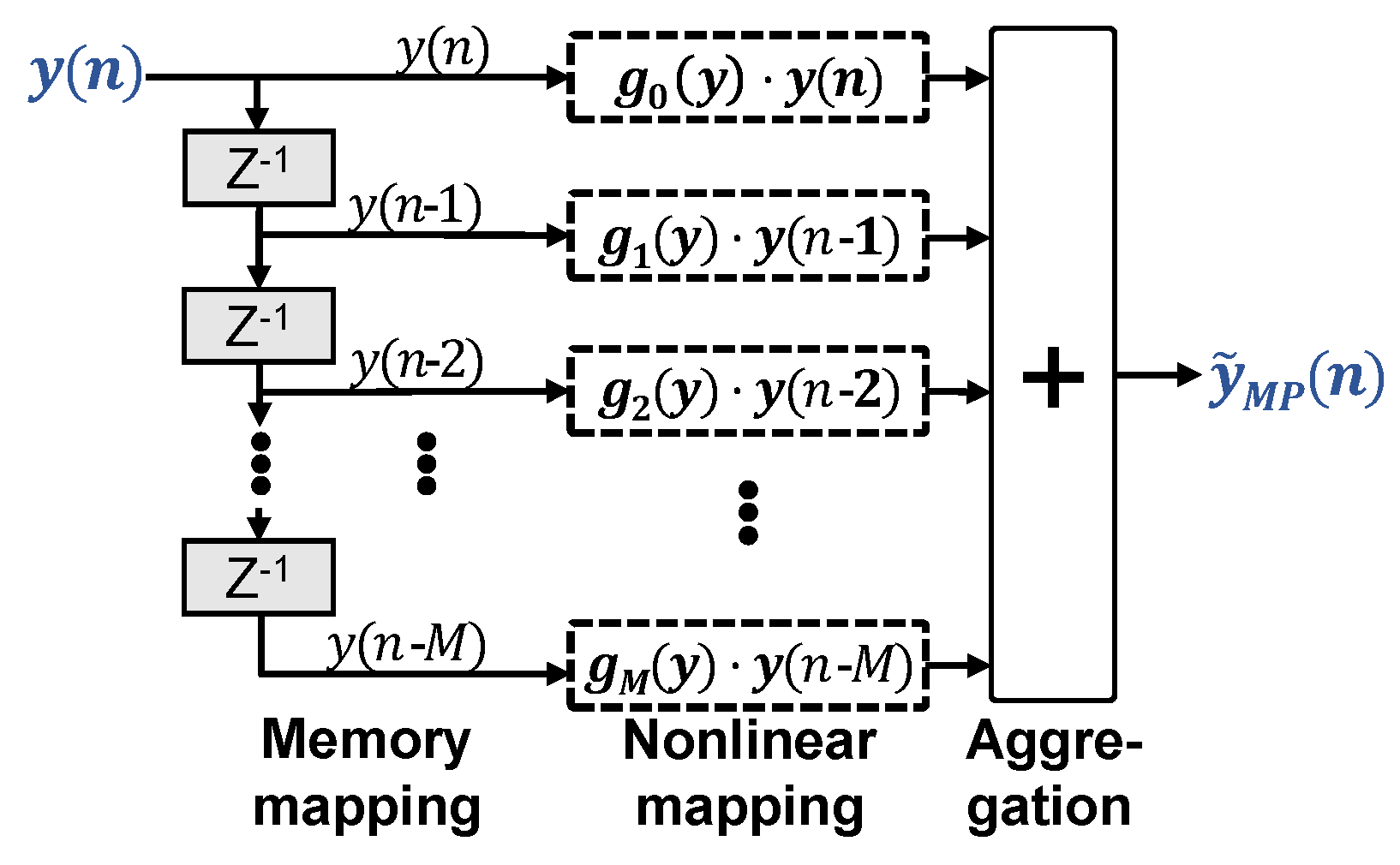
Figure 1 illustrates this mapping of memory and nonlinearity in respect to the input signal , which can be either real- or complex-valued. A VNLE architecture with given memory size and order is fully described by its so-called kernels . Before operation, they have to be identified, i.e., configured upon training data, in order to match the nonlinearities of interest. To this means, iterative approaches exist, such as least mean squares (LMS) or recursive least squares (RLS) kernel extraction. They are good solutions if little training data is available at a time or if channel dynamics call for frequent kernel reconfiguration. Typical O/E channels, however, are static enough to allow for a one shot configuration on a sufficiently large data set. The optimal solution in terms of the least squares (LS) error criterion to match the equalizer output to the desired signal (training signal) is achieved with a single operation LS solver. It involves inverting matrices, built from transmitted and received training data [9]. It has been shown [10] that these matrices can be ill-conditioned, resulting in a huge ratio between the highest and lowest eigenvalues. As a result, this matrix becomes nearly singular. With growing matrix complexity, i.e., increasing P or M, the inverse of the matrix is computed with less and less accuracy. This calls for a trade off between matrix conditioning and the number of kernels for maximum performance.

Figure 1.
General nonlinear volterra equalizer.
2.2. Memory Polynomial Volterra Equalizer
Shrinking the architectural complexity of VNLEs makes sense for two reasons. Less digital signal processing (DSP) resources are needed for deployment in actual transceivers and the LS matrices become less ill-conditioned. Figure 2 illustrates the MP-VNLE structure. MP-VNLEs prune general VNLEs simply by removing all cross terms generated by and its delayed versions :
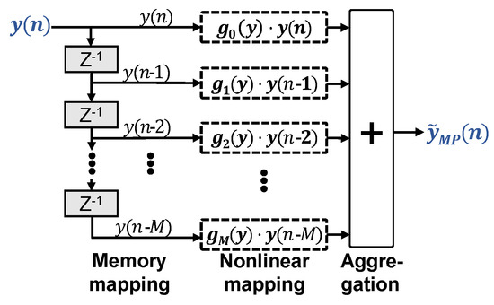
Figure 2.
Memory polynomial nonlinear equalizer.
One may rewrite this as
Given a memory tap m, becomes a constant gain to the memory term . , in turn, depends only on the polynomial power terms of . Again, can be real- or complex-valued.
2.3. Deep Neural Network Equalizer
Along with other science and engineering disciplines, the optical communication community is adopting ML for a broad range of problems [11,12,13]. Neural network (NN) is a subcategory of ML, which automatically learns systematic features within an arbitrary data set. It then can extract and extrapolate these features to new data.
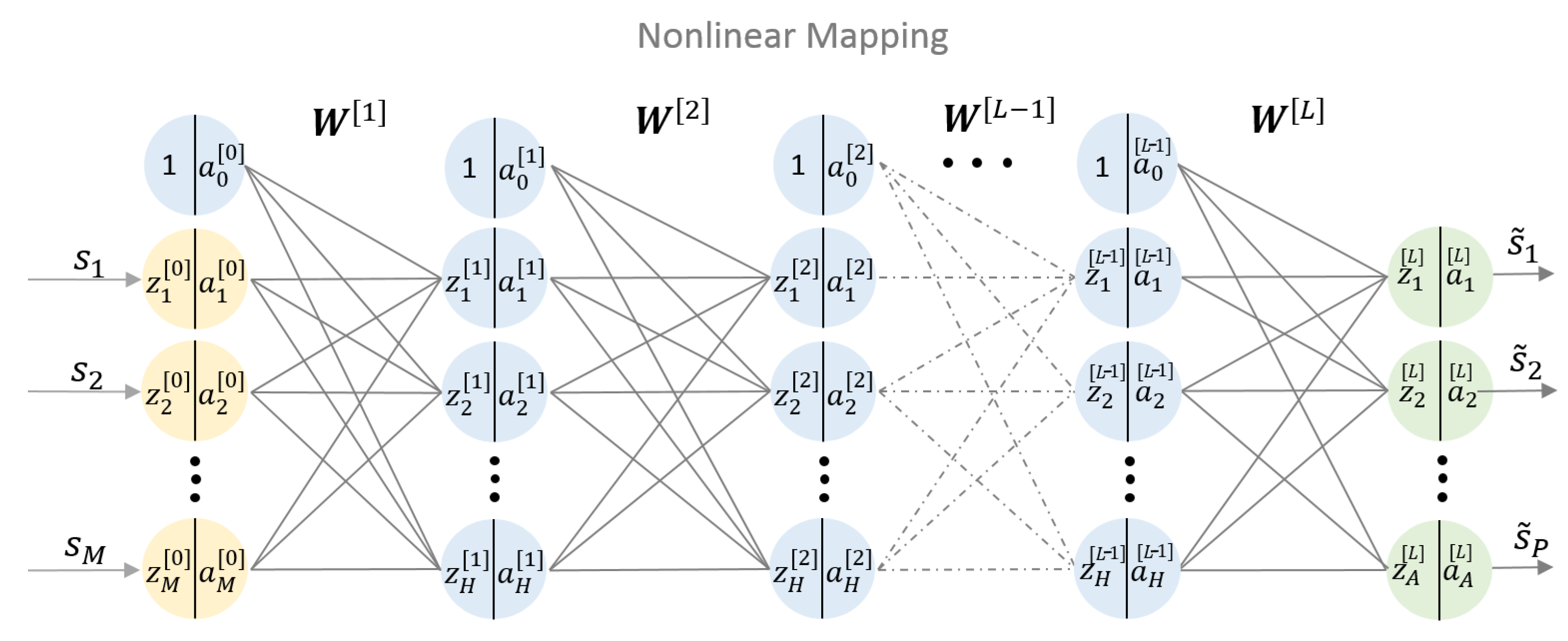
NNs computing structures are built from several layers of artificial neurons. A single artificial neuron is a processing unit with a number of inputs and one output. Each input is associated with a weight. The neuron firstly computes an activation by summing up the particular weighted inputs and a bias term. Secondly, an activation function is applied to obtain the neurons’s output . The neurons’s behaviour is defined by the weights, bias and the activation function [14]. Interconnecting multiple neurons builds a NN. If more than one hidden layer is used, the NN is called a deep NN, referred to as DNN. DNNs are convenient to model unknown highly complex relations. As such, they are capable of learning nonlinear equalization. In machine learning terms, nonlinear equalization can be treated as a problem of supervised nonlinear regression. A regression DNN learns a function by training on a dataset, where M is the input dimension and A is the output dimension. Figure 3 shows a basic architecture of a regressive neural network with multiple hidden layers. The bias term is included by an additional branch to each neuron. The notation is as follows [14]:
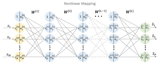
Figure 3.
L-layers feed-forward deep neural networks (DNN) with M nodes in the input layer, H nodes in the hidden layers and A nodes in the output layer.
- denotes the input signal,
- denotes the equalized signal,
- denotes a weight matrix (including the bias) between the -th layer to the l-th layer,
- denotes the output of the i-th neuron in the l-th layer,
- denotes the summed up input to the i-th neuron in the l-th layer,
- The activation function is the relation between and of the i-th neuron in the l-th layer,
where l denotes the current layer and H the number of nodes in the hidden layers. Using these notations the output can be expressed as follows [14],
where the first line, Equation (4), denotes the input layer and the second as well as the third lines, Equations (5) and (6), are executed iteratively for subsequent layers to obtain the output . For regression problems, the activation function in the last layer may differ from the activation functions used in the hidden layers. The hidden layers usually use nonlinear functions, while the type of activation function at the last layer should be matched to the application. This output activation function has to represent the overall dynamic range of the target signal. A common choice is therefore the identity activation function for a regression problem. The identity activation function is applied to each neuron at the output layer. The DNN models the relation of and as being an output of a DNN with respect to the input and the nonlinear functions. The equalized signal is obtained at the output of the DNN and can be expressed as follows,
In order to find the weights such that the outputs are close to the target outputs and to assess performance of the DNN, a cost function has to be introduced. The cost function is derived using the Maximum Likelihood principle. Considering the regression problem with the training data set of N inputs , along with the corresponding target output values ,
where each has M entries and each has A entries for all . The error between the DNN output and the target values is defined as
Using Equation (9) and assuming a Gaussian distribution of the error with zero mean and variance , as well as statistically independent symbols, the joint conditional probability density function can be derived,
According to the ML principle, our target is to find the Maximum Likelihood estimates of for the DNN which gives the highest probability of our training data. This can be done by maximizing the joint conditional probability density function Equation (10).
By applying the logarithm on Equation (11), we obtain the quadratic cost function. Thus, minimizing the quadratic cost function corresponds to finding the ML estimate of weights for the DNN. Equation (14) defines the final overall cost of all samples in the dataset. In order to find the weights, which minimize the quadratic cost function, the gradient descent algorithm [15] is used. Here, the gradients of the cost function have to be computed with respect to the DNN parameters. An efficient method is the common backpropagation algorithm [16]. The backpropagation algorithm approaches the derivatives of the cost function from the training set with respect to the network parameters. It applies the chain rule for derivatives very efficiently. The derivation of the cost function with respect to the weights in the Lth-layer down to the first layer by applying the chain rule, can be expressed as follows
The computation of the gradients in the previous layer build on the particular gradients in the post layer. Thus, some particular gradients of the expended chain rule expression have to be evaluated only once. Specifying Equations (15) and (16), by considering the quadratic cost function, the single gradients can be solved and simplified as [14]
where denotes the derivation of the activation function in the current layer. Equation (18) is executed iteratively for subsequent layers. The final gradients are used to update the weights by shifting the old weight values towards negative direction of the gradient, given by the Equation (19). The parameter denotes the learning rate and is adaptively adjusted by the adaptive moment estimation (ADAM) [15] in order to enable the gradient algorithm to move gently towards the global minimum.
3. Experimental Verification and Discussion
This section outlines the measurement setup, as used to evaluate the nonlinear compensation performance of the following four NLE architectures on basis of identical offline data: VNLE, MP-VNLE and two types of DNN-NLEs.
3.1. Measurement Setup
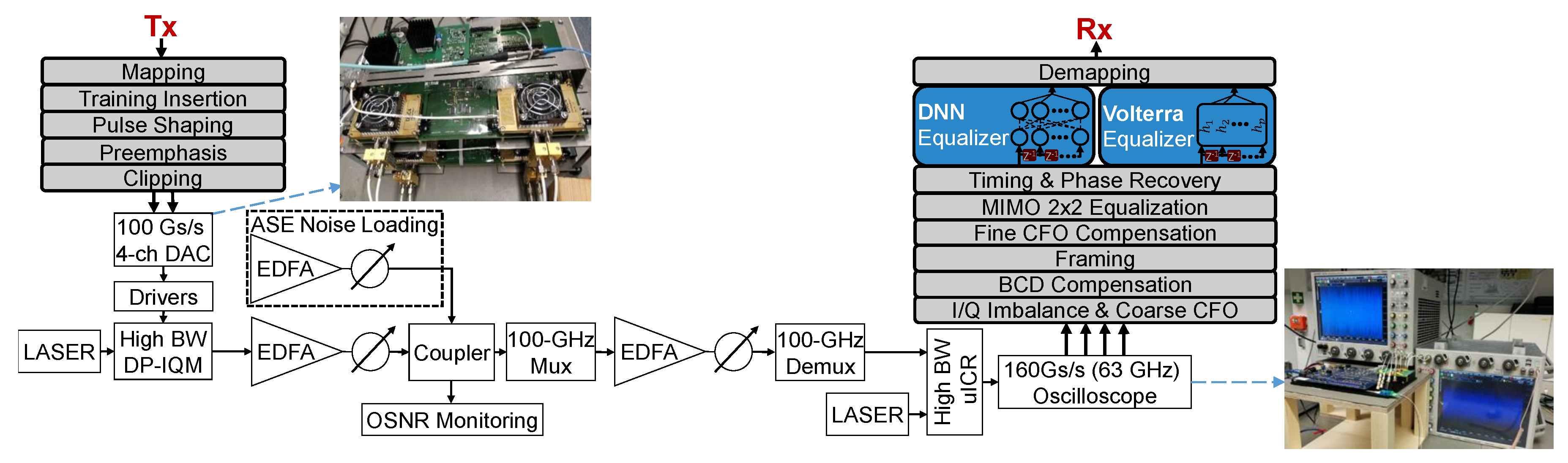
A coherent single carrier transmission system over a single mode fiber (SSMF) is employed to experimentally evaluate the performance of the proposed schemes. The dual polarization 600 Gb/s experimental setup including the offline DSP stack is shown in Figure 4. The measurements were performed BtB at 1550 nm with amplified spontaneous emission (ASE) noise loading, in order to compare bit error rates before applying any forward error correction (pre-FEC BER) at varying optical signal to noise ratios (OSNR). For a net bitrate of 600 Gb/s, 704 Gb/s of pseudo random data including overheads of FEC and training have been transmitted at 88 GBd for 16QAM, at 70 GBd for 32QAM and at 68 GBd for 64QAM.
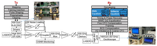
Figure 4.
Back-to-back offline measurement setup including Tx and Rx digital signal processing (DSP) with different methods to compute the L-values.
The photos show a VEGA 100 GSa/s 4-channel DAC by Micram with 40 GHz bandwidth and 4.5 ENOB and two 2-channel 160 GSa/s Keysight Infiniium oscilloscopes with 63 GHz bandwidth. Their nonlinear effects are mixed with nonlinear distortions from SHF 804 A drivers, a Fujitsu 64 GBd DP-IQM and a NeoPhotonics 64 GBd class-40 HB-ICR (40 GHz). Unlike in this BtB setup, longer fiber spans as well as a WDM-setup would introduce further nonlinearities, such as single, cross and multichannel nonlinear interferences.
The transmitter DSP inserts a CAZAC (constant amplitude zero autocorrelation) based training sequence. These training symbols are used for framing, carrier frequency offset estimation, 2 × 2 MIMO equalization and residual chromatic dispersion compensation. These sequences of 4096 training symbols are sent prior to more than payload data symbols repetitively. This makes it a minimal frame structure, of which the oscilloscope’s memory stores up to four per capture. The DSP uses a linear preemphasis filter on the TX side against linear O/E component distortions.
The receiver DSP stack includes classical signal recovery blocks [17,18]. The different NLEs are added after the timing and phase recovery and run at one sample per symbol. For fair performance comparisons, the different NLE types operate on identical power normalized data. Regardless of the type of NLE in use, training on the particular nonlinearities is essential before deployment. CAZAC sequences do not capture nonlinearities very well. Hence, NLE training is done instead upon the payload of the first captured frame for one of the OSNR captures. Once trained, the NLE can equalize all other captures without further training.
3.2. Measurement Results over an Optical Channel with 600 Gb/s/
For the ultimate goal of reaching 600 Gb/s net data rate with the lowest possible BER over a wide range of OSNR levels, an optimal combination of modulation scheme and baud rate needs to be chosen in a first step, before improving its performance further with nonlinear equalization. Figure 5 shows the hard-decision preFEC BER for different modulation schemes with varying noise loading without applying NLE compensation.
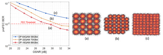
Figure 5.
Back to back 600 Gb/s (+15% FEC) measurements of different modulations without nonlinear equalizers (NLE).
The horizontal red dashed line indicates a typical FEC limit of . It can be observed that for the given setup, smaller constellation sizes improve performance much more than symbol rate reductions. DP-64QAM/58 GBd does not even reach the FEC threshold within the observed OSNR range without NLE. DP-16QAM/88 GBd proves to be the most performant scheme and thus, it is chosen for NLE architecture comparisons upon its offline data.
For fair comparisons, all options apply 4 memory taps. Per option, calibration is done exactly once on the first of four frames of the capture taken at 29.7 dB OSNR (calibration point). This ensures strict separation of calibration and measurement data, respectively training and testing data.
Figure 6 depicts the training and evaluation process. Each capture from the oscilloscope includes up to four frames, represented by the squares. For each capture the DAC is reloaded with pseudo random data. The blue square indicates the training data, while the green squares indicate the testing data. The gray colored frames are not used. For each OSNR value the overall BER is evaluated over four frames.
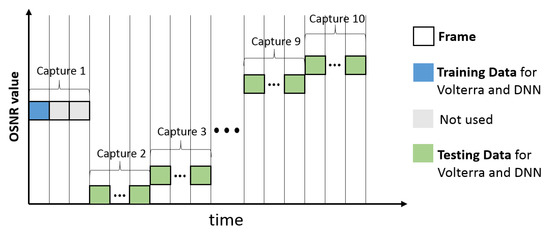
Figure 6.
Overview training and evaluation process.
3.2.1. General and Memory Polynomial (MP-) Volterra nonlinear Equalizer (VNLE)
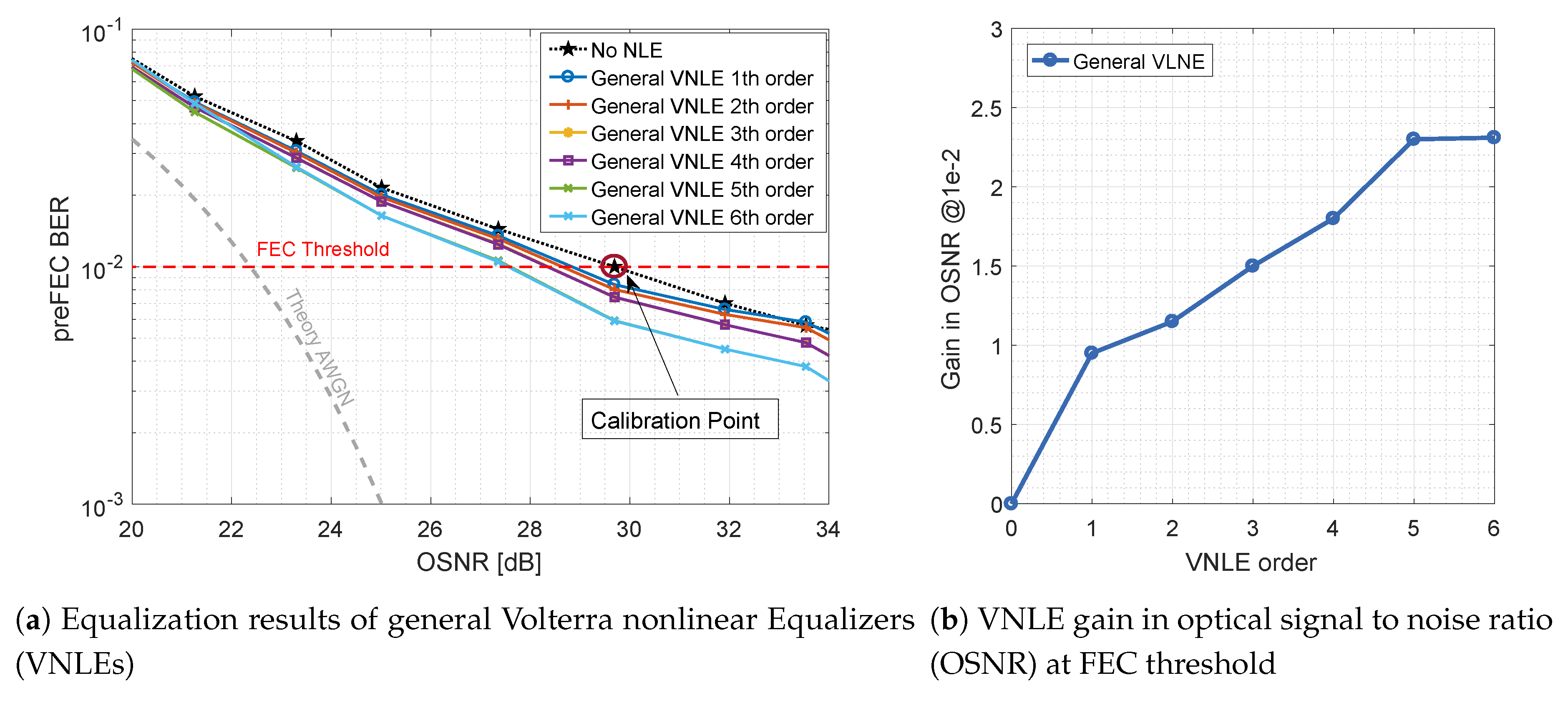
Figure 7 shows the performance improvement by applying general VNLE full kernel architectures of different orders. The gray dashed line depicts the theoretical upper limit for DP-16QAM at 88 Gbaud over an additive white Gaussian noise (AWGN) channel. The computational effort of a full kernel architecture gets extremely high with rising orders. Thus, only up to 6th order kernels are considered and evaluated. On the left hand side, Figure 7a plots the preFEC BER related to the OSNR. On the right hand side, Figure 7b shows the improvements of these base-line curves. The gains in OSNR at their crossing with the FEC threshold are plotted against the order. The general VNLE of 5th order improves the non-equalized baseline curve by 2.3 dB at a target FEC BER of . Increasing the VNLE order further to 6th order does not yield significant additional gain.
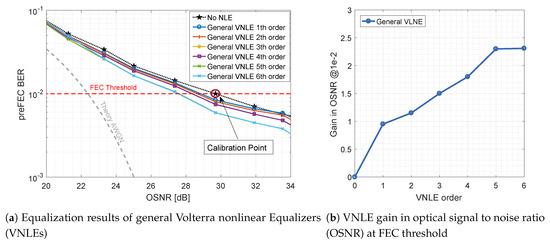
Figure 7.
Optical back-to-back 600 Gb/s/λ general VNLE preFEC measurement results.
Figure 8a shows the performance of the reduced size alternative, the MP-VNLE, which operates only on subset of kernels. As before, the performance was evaluated for different maximum polynomial orders. In comparison to the general VNLE, the architecture of the MP-VNLE is less complex and hence the computational effort to evaluate the kernels is lower. Therefore, higher orders are applicable for real systems. The MP-VNLE of 5th order improves the baseline curve by 2.0 dB at the FEC threshold of shown in Figure 8b. It can be observed, that the reduction costs performance of 0.3 dB and that higher orders do not improve the performance. On the contrary, the performance is rather inferior. This indicates that the higher order computations lead to numerical instability when identifying and extracting the VNLE kernels with the least squares (LS) solver approach. However, besides the numerical instability such high orders are out of scope due too high implementation complexity.
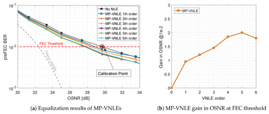
Figure 8.
Optical back-to-back 600 Gb/s/λ MP-VNLE preFEC measurement results.
3.2.2. Deep Neural Network Equalizer
While the LS-solver calibrates (MP-)VNLE kernels in a single shot, the weights and biases for DNN-NLE are trained in numerous iterations (epochs). The weights and biases of the DNN-NLE are updated by shifting the previous values towards the negative direction of the gradient. Therefore, the mini-batch backpropagation algorithm, which computes the gradients of the cost function in respect to the network parameters, and the stochastic gradient descent optimizer ADAM are applied. The hyper parameters are constant for all structures. The mini-batch size is set to of the numbers of symbols of the training frame, respectively to symbols. The learning rate of the ADAM optimizer is set to , which is a common value. In order to prevent overfitting, the performance of the DNN is repetitively validated on testing data during the training phase.
The design options for DNN-NLEs are numerous and interrelated. There are no rules for the number of layers or neurons per layer to model a given problem. The more neurons the network interconnects, the finer the modeling capabilities become. More complexity, however, makes DNNs prone to overfitting [19]. Figure 9 shows two DNN equalizer architectures with multiple hidden layers and extra input nodes in order to consider the channel memory effects. On the left hand side, four separate DNNs are depicted with one output node for handling the inphase and quadrature components and polarization independently. On the right hand side, a DNN structure is shown that handles the inphase and quadrature for each polarization jointly. In principle, the joint option could learn as well nonlinear phase impairments in addition to nonlinearities. In both cases, the input nodes feed and as well as and . Memory effects of channel and components are considered by adding time delayed versions of the input signal. The memory depth is defined by the parameter M and is set to 4, equal to the previous setting of the Volterra equalizers. The number of hidden layers layers and the corresponding number of neurons per layer of the particular networks were varied during the examination. In order to compare learning speed and performance. Table 1 list the different structures, where the last column represents the total number of independent hardware multpliers to process the data stream of two polarizations. Regardless of the structure, for the hidden neurons as well as for the output neurons a tanh has been chosen as activation functions. The design e.g., stands for 5 input neurons (input signal + 4 memory taps) followed by three hidden layers with 20, 30 and 40 neurons, feeding into 1 output node. The higher the number of layers and neurons, the higher the computational effort and hence the complexity.
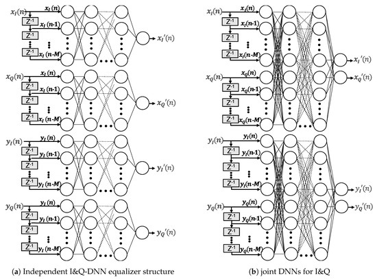
Figure 9.
Deep Neural Network Equalizer Architectures.

Table 1.
DNN structures.
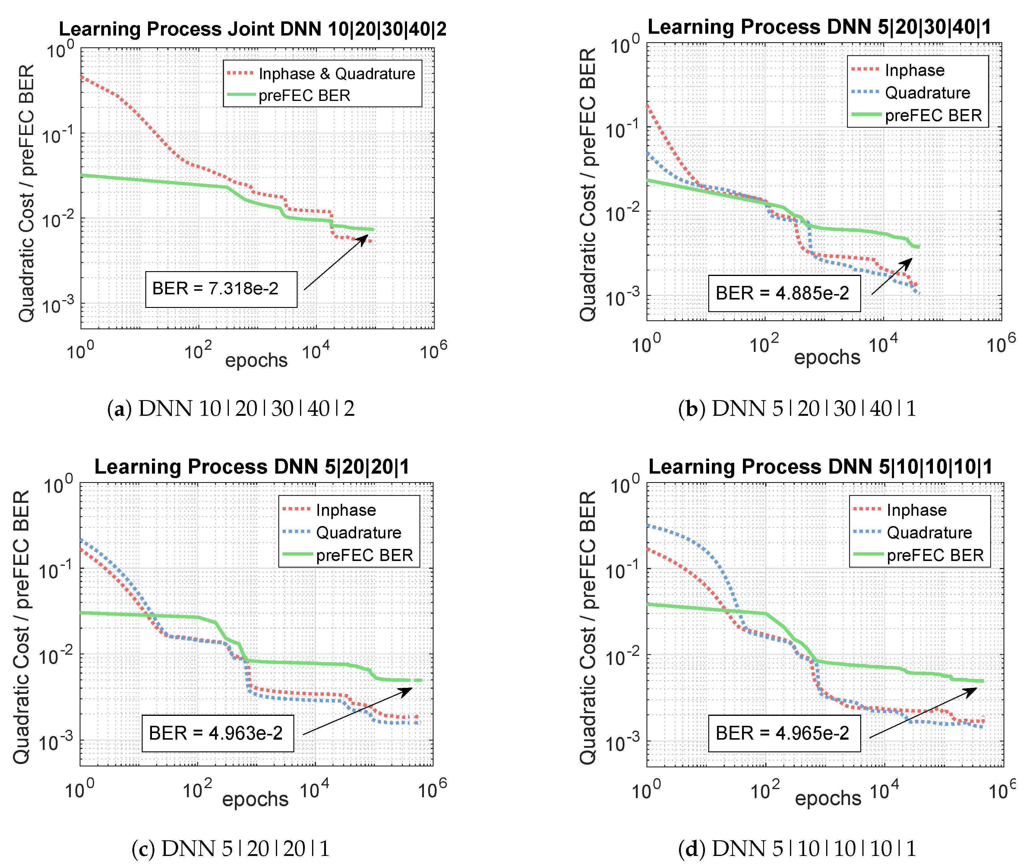
Figure 10 shows the learning process of the four different independent I&Q-DNN equalizer structures for the optical BtB 600 Gb/s measurements. The blue and the red dashed curves indicate the cost functions, given by Equation (14), of the inphase and quadrature components for one polarization, while the green curves represent the preFEC BERs related to numbers of epochs. It can be observed, that the most complex design, shown in Figure 10b converges the fastest. The learning speed of the structures depicted in Figure 10a,c,d is slightly slower, especially at the beginning. However, all options need at least around epochs for learning the component nonlinearities. The long training process is one disadvantage of the neural network equalizer and calls for further improvement and research.
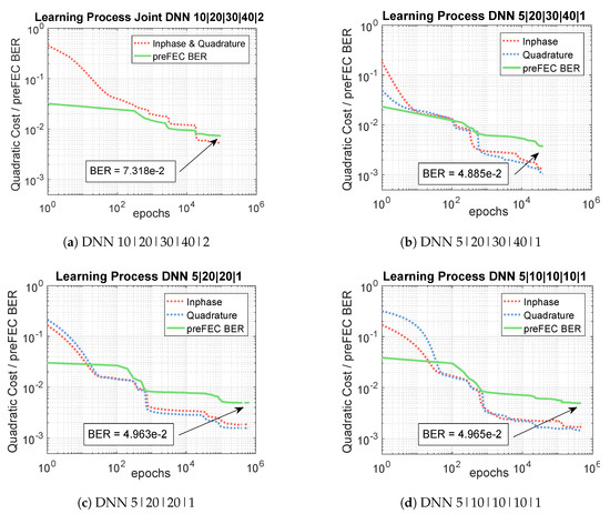
Figure 10.
Learning Process of three different DNN structures.
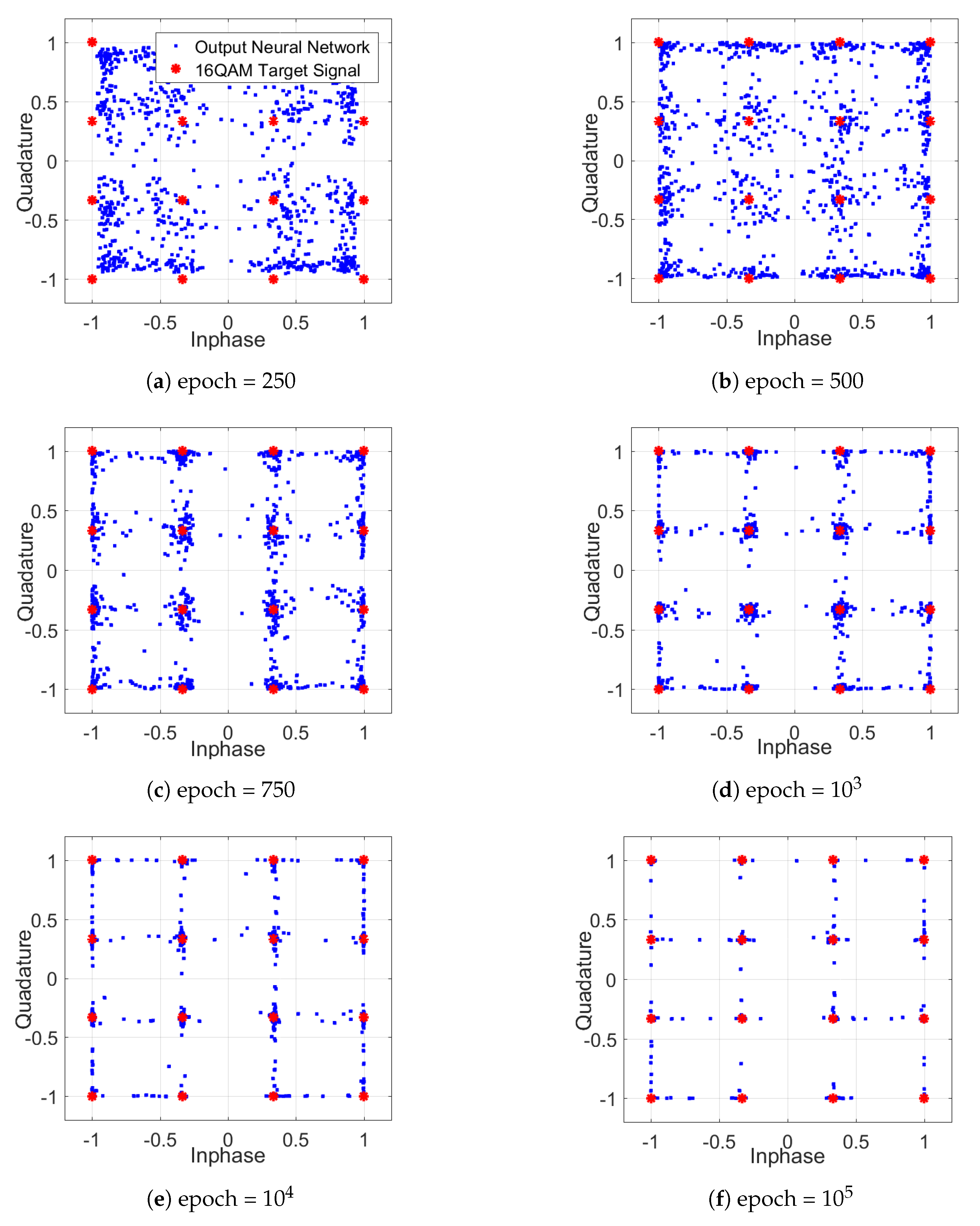
In addition to the learning behavior, Figure 11 shows the altered constellation diagrams of the equalized signal for one polarization during the training of the DNN NLE. The resulting constellations, such as the one in Figure 11f, differ fundamentally from a classical constellation. The DNN-NLE has the ability of concentrating the constellation points and to reduce the possible outputs (dimensional space) to the target 16QAM points, in order to reach a low value of the cost function. In combination with the tanh activation function, a square grid constellation occurs, which exhibits non-Gaussian distributed noise.
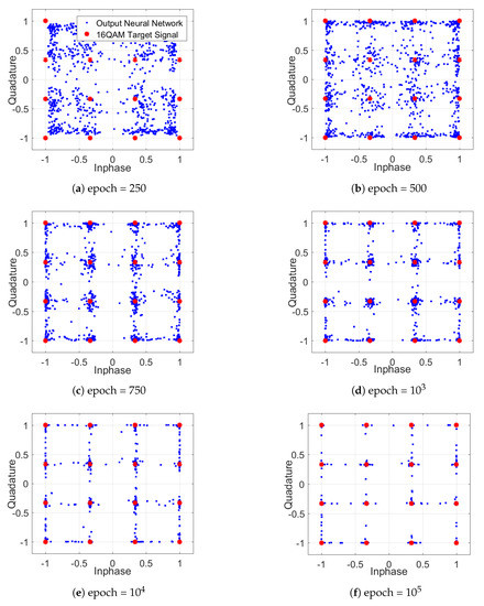
Figure 11.
Constellation diagrams during the learning process.
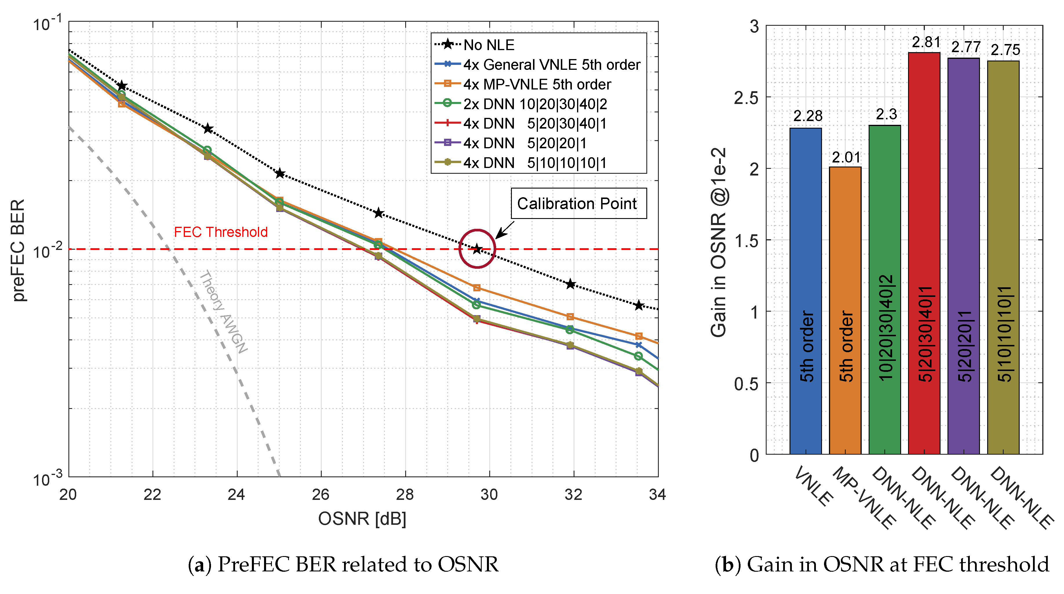
The overall performance of the DNN-Equalizer is shown in Figure 12. On the left hand side, Figure 12a plots the preFEC BER as a function of the OSNR, comparing the best performing general VNLE of 5th order, the best performing reduced size alternative MP-VNLE of 5th order and the proposed DNN-NLE structures. On the right hand side, Figure 12b shows the improvements of the base-line curve. The gains in OSNR at the FEC threshold are plotted. The most complex DNN design, which processes I and Q separately, performs best. This architecture improves the base line curve by 2.81 dB and outperforms the 5th order VNLE and MP-VNLE by 0.53 dB and 0.80 dB, respectively. The performance losses of the lower complex and designs are very low. The performance is almost identical to the much larger design. The design with joint processing, performs worst among all DNN structures. The higher number of input nodes together with the equal number of neurons in the hidden layers as the independent I and Q equalizer structure leads to suboptimal projection of the input signal.
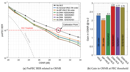
Figure 12.
Optical Back-to-Back 660 Gb/s/λ postFEC BER measurements results applying different Volterra and deep neural network architectures.
Fair complexity comparisons are not trivial. Given 4 memory taps, a 5th order MP-VNLE requires 25 kernels, a general VNLE 3905 kernels [8]. However, most of these VNLE kernels can be safely pruned without severe performance reduction [20]. The DNN-NLE requires 291 trainable parameters (weights, biases), respectively 1040 independent hardware multipliers, which can be pruned considerably, too [21]. Besides the sheer number of trainable parameters, the way of using them for polynomials or activation functions is of course decisive, too.
4. Conclusions
The algorithmic deficits in kernel identification for Volterra nonlinear equalizers and their general large architectural complexity have motivated investigations in deep neural network nonlinear equalizer alternatives. In coherent 88 Gbaud DP-16QAM 600 Gb/s measurements, deep neural network nonlinear equalizers proved to reflect systematic nonlinearities more accurately than 5th order memory polynomial and full kernel Volterra nonlinear equalizers. They outperform by 0.5 dB and 0.8 dB, respectively. Based on back-to-back measurements, where optical and electrical components nonlinearities predominate. The disadvantages of deep neural network nonlinear equalizers include their vast parameter space, which is hard to manage and their long training process. While this article highlights performance gains of DNN NLEs over classical Volterra schemes, their implementation complexity has yet to be compared in greater detail in future work, in order to demonstrate its overall superiority.
Author Contributions
Conceptualization, M.S., C.B., M.K. and S.C.; Data curation, C.B. and F.P.; Formal analysis, M.S.; Methodology, M.S.; Resources, F.P.; Software, M.S.; Supervision, M.K.; Visualization, M.S. and C.B.; Writing—original draft, M.S. and C.B.; Writing—review & editing, M.K., C.B., M.K., S.C. and S.P.
Funding
This research received no external funding.
Conflicts of Interest
The authors declare no conflict of interest.
References
- Bluemm, C.; Schaedler, M.; Kuschnerov, M.; Pittala, F.; Xie, C. Single Carrier vs. OFDM for Coherent 600Gb/s Data Centre Interconnects with Nonlinear Equalization. In Proceedings of the 2019 Optical Fiber Communications Conference and Exhibition (OFC), San Diego, CA, USA, 3–7 March 2019. [Google Scholar]
- Amari, A.; Dobre, O.A.; Venkatesan, R.; Kumar, O.S.; Ciblat, P.; Jaouen, Y. A survey on fiber nonlinearity compensation for 400 Gb/s and beyond optical communication systems. IEEE Commun. Surv. Tutor. 2017, 19, 3097–3113. [Google Scholar] [CrossRef]
- Rezania, A.; Cartledge, J.C.; Bakhshali, A.; Chan, W.Y. Compensation schemes for transmitter-and receiver-based pattern-dependent distortion. IEEE Photonics Technol. Lett. 2016, 28, 2641–2644. [Google Scholar] [CrossRef]
- Cartledge, J.C. Volterra Equalization for Nonlinearities in Optical Fiber Communications. In Signal Processing in Photonic Communications; Optical Society of America: Washington, DC, USA, 2017. [Google Scholar]
- Schetzen, M. Theory of pth-order inverses of nonlinear systems. IEEE Trans. Circuits Syst. 1976, 23, 285–291. [Google Scholar] [CrossRef]
- Kim, J.; Konstantinou, K. Digital predistortion of wideband signals based on power amplifier model with memory. Electron. Lett. 2001, 37, 1417–1418. [Google Scholar] [CrossRef]
- Kamalov, V.; Jovanovski, L.; Vusirikala, V.; Zhang, S.; Yaman, F.; Nakamura, K.; Inoue, T.; Mateo, E.; Inada, Y. Evolution from 8QAM live traffic to PS 64-QAM with neural-network based nonlinearity compensation on 11000 km open subsea cable. In Proceedings of the Optical Fiber Communication Conference, San Diego, CA, USA, 11–15 March 2018. [Google Scholar]
- Guan, L. FPGA-based Digital Convolution for Wireless Applications; Springer International Publishing: New York, NY, USA, 2017. [Google Scholar]
- Ghannouchi, F.M.; Hammi, O.; Helaoui, M. Behavioral Modeling and Predistortion of Wideband Wireless Transmitters; John Wiley and Sons: Hoboken, NJ, USA, 2015. [Google Scholar]
- Raich, R.; Zhou, G.T. Orthogonal polynomials for complex Gaussian processes. IEEE Trans. Signal Process. 2004, 52, 2788–2797. [Google Scholar] [CrossRef]
- Musumeci, F.; Rottondi, C.; Nag, A.; Macaluso, I.; Zibar, D.; Ruffini, M.; Tornatore, M. An overview on application of machine learning techniques in optical networks. IEEE Commun. Surv. Tutor. 2018, 21, 1383–1408. [Google Scholar] [CrossRef]
- Khan, F.N.; Fan, Q.; Lu, C.; Lau, A.P.T. An Optical Communication’s Perspective on Machine Learning and Its Applications. J. Light. Technol. 2019, 37, 493–516. [Google Scholar] [CrossRef]
- Schaedler, M.; Kuschnerov, M.; Pachnicke, S.; Bluemm, C.; Pittala, F.; Changsong, X. Subcarrier Power Loading for Coherent Optical OFDM optimized by Machine Learning. In Proceedings of the Optical Fiber Communication Conference, San Diego, CA, USA, 3–7 March 2019. [Google Scholar]
- Bishop, C.M. Pattern Recognition and Machine Learning; Springer: New York, NY, USA, 2006. [Google Scholar]
- Kingma, D.P.; Ba, J. Adam: A method for stochastic optimization. arXiv 2014, arXiv:1412.6980. [Google Scholar]
- Hecht-Nielsen, R. Theory of the backpropagation neural network. In Neural Networks for Perception; Academic Press: Cambridge, MA, USA, 1992; pp. 65–93. [Google Scholar]
- Pittalà, F.; Cano, I.N.; Bluemm, C.; Schaedler, M.; Calabrò, S.; Goeger, G.; Brenot, R.; Xie, C.; Shi, C.; Liu, G.N.; et al. 400Gbit/s DP-16QAM Transmission over 40km Unamplified SSMF with Low-Cost PON Lasers. IEEE Photonics Technol. Lett. 2019, 1, 1229–1232. [Google Scholar] [CrossRef]
- Gao, Y.; Lau, A.P.T.; Lu, C.; Wu, J.; Li, Y.; Xu, K.; Li, W.; Lin, J. Low-complexity two-stage carrier phase estimation for 16-QAM systems using QPSK partitioning and maximum likelihood detection. In Proceedings of the 2011 Optical Fiber Communication Conference and Exposition and the National Fiber Optic Engineers Conference, Los Angeles, CA, USA, 6–10 March 2011. [Google Scholar]
- Goodfellow, I.; Bengio, Y.; Courville, A. Deep Learning; MIT Press: Cambridge, MA, USA, 2016. [Google Scholar]
- Huang, W.J.; Chang, W.F.; Wei, C.C.; Liu, J.J.; Chen, Y.C.; Chi, K.L.; Wang, C.L.; Shi, J.W.; Chen, J. 93% complexity reduction of Volterra nonlinear equalizer by L 1-regularization for 112-Gbps PAM-4 850-nm VCSEL optical interconnect. In Proceedings of the 2018 Optical Fiber Communications Conference and Exposition (OFC), San Diego, CA, USA, 11–15 March 2018. [Google Scholar]
- Han, S.; Mao, H.; Dally, W.J. Deep compression: Compressing deep neural networks with pruning, trained quantization and huffman coding. arXiv 2015, arXiv:1510.00149. [Google Scholar]


© 2019 by the authors. Licensee MDPI, Basel, Switzerland. This article is an open access article distributed under the terms and conditions of the Creative Commons Attribution (CC BY) license (http://creativecommons.org/licenses/by/4.0/).