Featured Application
In this paper, the innovative use of a multiscale flow-focused geographically weighted regression (MFGWR) approach to model the spatial interaction of expressway transport flow is critically evaluated. The study demonstrates varied scale effects between push and pull forces and provides datadriven evidence to inform transport planning, infrastructure construction and economic development at a regional level.
Abstract
Scale is a fundamental geographical concept and its role in different geographical contexts has been widely documented. The increasing availability of transport mobility data, in the form of big datasets, enables further incorporation of spatial dependencies and non-stationarity into spatial interaction modeling of transport flows. In this paper a newly developed multiscale flow-focused geographically weighted regression (MFGWR) approach has been applied, in addition to global and local Moran I indices of flow data, to model multiscale socio-economic determinants of regional transport flows between counties across the Jiangsu Province in China. The results have confirmed the power of local Moran I of flow data for identifying urban agglomerations and the effectiveness of MFGWR in exploring multiscale processes of spatial interactions. A comparison between MFGWR and flow-focused geographically weighted regression (FGWR) showed that the MFGWR approach can better interpret the heterogeneous processes of spatial interaction.
1. Introduction
Since the end of the 20th century, with the increasing development of globalisation and informatisation, the flow of various elements (people, goods, knowledge and information) has become more frequent across various scales, and accordingly, regions have become the space of flows [1]. In this context, the concept of space of flows is gradually replacing the space of place [2]. Mobilities have become a hallmark of modern times [3]. The emergence of flow space has had a disruptive impact on space-distance-based and cored geography [4]. Regional spatial morphology is also being redefined and modified as researchers from multiple disciplines have begun to recognize and analyse spatial structure using the flow rather than central place perspective [5]. As the most important form of spatial interaction to connect and increase communication between different geographical spaces, transport flow undoubtedly has remarkable impacts on economic activity space and is a key factor in the shaping of socio-economic spatial structure [6]. Understanding these impacts has wider significance for interpreting the spatial distribution law of various economic phenomena [7].
With the increasing demand for fast inter-city transport, the infrastructure including expressways, airlines, high-speed railways and ETC (Electronic Toll Collection) systems have become the most important parts of the modern transport system [8]. As such, the transport flows over the network of these infrastructure systems have been widely studied. The regional transport flow on well-networked expressways has contributed remarkably to the socio-economic links between large and medium cities [9], particularly in view of the spatial interactions [10]. Compared with the air and railway networks, the expressway network has its own unique characteristics. Firstly, the flow pattern is much more complex due to high frequency and dynamics, which results in spatial heterogeneity [8]. Secondly, the transport flow on such network is more fragile and vulnerable to many physical and human factors (e.g., weather, accidents and regulations), it can be envisioned that its spatial interaction patterns have strong economic and demographic effects and implications for policy-making [11]. Thirdly, such a pattern with the mixture of long- and short-distance flows across the region indicates varied levels of urban agglomeration [12].
In the field of geographical mobility, there is a long history of deploying a gravity model to analyse the spatial economic interactions between cities and regions by considering a variety of physical, social, economic and even environmental dimensions [13,14]. The traditional methods of calibrating the spatial interaction models are dominated by global regression models (e.g., Ordinary Least Square (OLS), Poisson Regression and negative binomial regression) based on the assumption that the mobility pattern is spatially stationary. However, the socio-economic systems driving the transport flows at a regional scale demonstrate heterogeneous density, intensity and diversity. This has resulted in the development of flow models by considering spatial heterogeneity, which will be calibrated by local regression methods. There is a recent development of such local regression methods in geography in considering spatial non-stationarity, among which geographically weighted regression (GWR) has become one of most popular approaches [15]. The extension of GWR into flow modelling was initiated by the seminal paper of spatially weighted interaction models (SWIM) [16]. This modelling method was upgraded to geographically weighted negative binomial regression (GWNBR) [17]. In parallel, the flowAMOEBA method, based on a multidirectional optimum ecotope-based algorithm, is able to analyse flow patterns through defining a spatial flow neighborhood [18]. However, the classic GWRs, using multiple explanatory variables, assume that all the explanatory variables have a spatially homogeneous process of determining the pattern of a dependent variable, or simply speaking, operate on a single spatial scale. Scale is a fundamental geographic concept, and the role it plays in different geographical contexts and processes has been documented extensively [19,20]. Therefore, a new multiscale geographically weighted regression (MGWR) was proposed and developed in the innovative work [21]. The MGWR method allows for the conditional relationship between response (dependent) variable and the variation of explanatory variables at different spatial scales. That is to say, each variable changes on the surface of the parameter to allow different bandwidths to be represented. Technically, MGWR minimizes overfitting by eliminating the limitations of all relationships varying on the same spatial scale, reducing bias and collinearity in parameter estimation [21,22,23,24]. Therefore, when using flow focused GWR (FGWR) to explore multi-scale spatial heterogeneity in flow patterns, MGWR has become the most ideal local model specification [25]. Compared with the classic GWRs, the MGWR parameter estimates are more accurate and more intuitive [21]. Since the MGWR method currently only supports point/polygon data-based modeling, the aim of this paper is to extend MGWR and apply it to the modeling of spatial interaction data.
Methodologically, the specific spatial relationship between flows is measured by flow-oriented spatial weight based on the Euclidean distance between flows as directed lines. The multiscale flow-focused geographically weighted regression model (MFGWR) is an extension of spatial interaction modelling and multi-scale geographically weighted regression (by considering multi-scale effects in the spatial non-stationarity of flows). This paper reports the first empirical study of multi-scale flow modelling applied for regional transport flows across the Jiangsu province in China. The contribution of this innovative method will be critically evaluated as well. This paper is organized as follows. Section 2 describes the study area, data collection and potential determinants of flow variations. Section 3 explains the modelling methods of MFGWR. Section 4 presents the modelling results and interpret the empirical study. The final section draws general conclusions, discusses limitations and makes recommendations for future work.
2. Study Area and Data Sources
2.1. Study Area
Jiangsu Province is located in the Yangtze River Delta and covers an area of 102,600 square kilometres (Figure 1). By the end of 2014, the population was over 76 million. This province is located in the most economically developed region of the country and is the fastest-growing province. Around the Yangtze River, Jiangsu is divided into three major regions, namely the Southern, the Central and the Northern, and the economic development between the north and the south is uncoordinated. Particularly, the Southern part, popularly called SuNan, has become a model of economic growth in China. The density of the expressway network across Jiangsu ranked the first in China in 2015 [26].
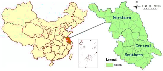
Figure 1.
Study area (Jiangsu province) and spatial units of county.
2.2. Data
2.2.1. Data Collection
The data sets for this case study include: OD transport flows between tollgates on the expressway network, toll gate locations and county-level socioeconomic data. There were 334 expressway tollgates throughout the Jiangsu Province. The OD transport flows between all 334 tollgates were processed from the transaction records of each tollgate. Each transaction record contains the vehicle ID and the time the vehicle entered or exited the tollgate. There were only two records per car—one for each entry to the tollgate and one for the exit tollgate. These two records define the individual OD travel of the vehicle. There were 235 million individual OD trips between these tollgates in 2014.
Administrative units in China were mainly composed of provinces, prefectures and counties. The county-level unit was the smallest spatial unit in the national socio-economic census surveys. In order to model the interdependence between transport and economy on a regional scale, it was necessary to summarize the transport flow at the county level. There were 63 counties in the Jiangsu Province, but this study only included 59 counties. This is because there were no transactions in four counties (Rudong, Funing, Jinhu and Gaochun) in 2014. The total transport volume at the county level during the year was processed into a 59 × 59 flow matrix. Relevant socioeconomic statistics were from Jiangsu Statistical Yearbook 2015 [27].
2.2.2. Flow Patterns
There were 3481 routes (= 59 × 59) between 59 counties (Figure 2). Statistically, the average transport flow between counties was 67,256.29 and the standard deviation was 424,074.9. A small number of transport flows (less than 100,000) were mainly located in northern Jiangsu, while a large number of transport flows were mainly concentrated in southern Jiangsu, which are mainly from Nanjing, Wuxi and Suzhou to the surrounding areas. Part of the transport connecting Xuzhou, Huai’an and Yancheng regional central cities contains more than 100,000 transport flow data. Among all transport flows, there were 10 traffic routes with more than 3 million flows, accounting for 24.43% of the total transport flows, dominating the expressway network. There were 32 traffic routes between 1 and 3 million, accounting for 21.47%. There are 2214 smaller routes (less than 10,000), accounting for only 2.71% of the total transport flows. The county-level network in southern Jiangsu was mainly composed of a small amount of high-volume, and the distribution of transport flow in the entire study area was obviously unbalanced.
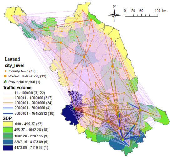
Figure 2.
Volume of transport flows on the expressway network at county level.
2.2.3. Explanatory Variables
Economy, population and distance have been proven to be the most important factors in driving geographical mobility (such as migration [28], tourism [29] and commuting [30]). In this study of regional mobility, the total population in the origin county was treated as a pushing force. Also, the GDP was selected as a pulling force in the destination county as a higher GDP generates more economic activity. Distance, in this case, the road network distance, is a spatial barrier for movement. The spatial distributions of GDP at the county level are displayed in Figure 3. The distance between counties was measured using Baidu maps, and its histogram displayed in Figure 3c. Traffic volume data between counties is shown in Table 1.
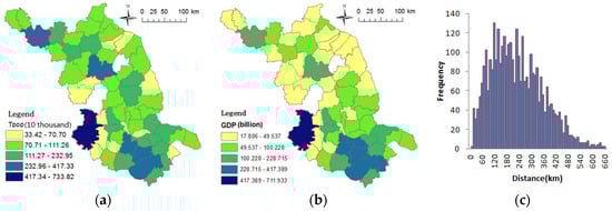
Figure 3.
Spatial distributions of pushing (Tpop) (a) and pulling force (GDP) (b) and the histogram of distance (c).

Table 1.
Explanatory variables of spatial interaction modelling.
3. Methodology
3.1. Flow Distance
Due to the complexity of flow data involving both origin and destination sites, flow modelling is needed to accurately measure the distance between OD flows. In contrast to the distance between points or polygons, the Euclidean distance between two flows ij and i′j′ (Figure 4) is measured as d(ij)(i′j′) (Equation (1)), in which the direction of flow is considered:
where and are the flow lengths. Using only the location information of the endpoint may sometimes be insufficient because the flow not only represents the interaction or movement between the two locations, but also the distance and direction in which the interaction or movement occurs [31]. Ref. [31] proposed an adjusted OD distance algorithm called Flow Dissimilarity (FDS) as follows (Equation (2)).
where is the Flow Dissimilarity between the two flows; and are the flow lengths. FDS is a scalar distance. The coefficients α and β are used to control the relative importance of the end points of the two OD flows (α + β = 2, α > 0, β > 0, default α = β = 1). In the case of transport flows, set α = β = 1. Besides the endpoint position and flow length, another spatial element of the flow is its directionality. However, in the case of transport flows, the influence of the direction on the weight is not taken into consideration.
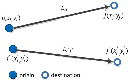
Figure 4.
The Euclidean distance between flow(ij) and flow().
3.2. Flow-Focused Global and Local Moran Indice
Global and local Moran Indices have become popular methods for measuring spatial autocorrelation, which is a form of spatial dependence. In this case study, both indices were employed for two purposes: detecting clustering patterns and defining clusters of flow, and examining the reduction of spatial auto-correlation in the residuals of global and local models of transport flows. The calculation of spatial autocorrelation depends on spatial weights. The distance threshold method is commonly used in the calculation of spatial weights.
Considering the unique spatial dependence of flows, spatial weight is defined by the spatial distance between OD flows [31]. Equation (3) is used to calculate the spatial distance between flows. Adjacent OD flows within a specified critical distance will be given a weight and have a significant impact on the calculation of the target OD flow. Adjacent OD flows that exceed a specified critical distance will be assigned a weight of zero and will not have any effect on the calculation of the target OD flow. The calculation method of the space weight is called the fixed distance band, and its equation is as follows:
where b is the fixed distance band, which should satisfy the requirement of ensuring at least one adjacent flow for each flow, and is the spatial distance between flow i and flow j. The Global Moran Indice is used to detect the pattern of transport flows: random, dispersed or clustered. The Local Moran Indice enables flows to be classified into four categories: HH (high-high), LL (low-low) and LH (low-high) and HL (high-low). HH means high volumes of flows are surrounded by a high volume of flows, and are therefore recognized as a hot cluster. Conversely, LL defines a cold cluster. LH and HL are defined as spatial outliers.
3.3. Multiscale Flow-Focused Geographically Weighted Regression
Spatial interaction modelling has been widely deployed to analyze various geographic mobilities (e.g., commuting, travel and migration). Currently, geographically weighted regression (GWR) [15,32] is the most commonly used model for geographical-weighted regression analysis. In this paper, the MGWR model was applied to the modelling of transport flow for the first time.
A simplified form of spatial interaction model is represented as follows (Equation (4)).
where is the interaction intensity between i and j, and represent the push and pull forces at the origin place i and destination place j respectively, denotes the distance between places i and j, and is a distance decay function of . In practice, and are often replaced by the scale of two places, e.g., population of origin and GDP of destination. Many studies argue that the distance decay function varies with spatial scales [26]. The non-linear functions of quantifying the distance decay effect are dominated by an inverse power function and a negative exponential function. The former is more suitable for analyzing short distance interactions on the urban scale and the latter more suitable for analysing longer distance interactions (such as migration flow) on regional or national scales [33]. For example, at urban scales, this distance decay function is often expressed as an inverse power function, which is evidentially confirmed by ref. [26]. At the regional scale (e.g., province in this study) the function is better expressed as negative exponential function (e.g., ), where β is the distance friction coefficient. The higher the value of β is, the more sensitive to distance the flow is.
In the case of transport flows at county level across a province, the pushing force at the county of origin is represented by its total population, , and the pulling force at the destination county by its total GDP, . A negative exponential function is suitable for the distance decay at the regional scale. The expressway network distance used for this case study was calculated using ArcGIS 10.5 Network Analyst.
The global model based on transport flow space interaction data is as follows (Equation (5)).
where k is the estimated intercept, α, β and γ are the parameters to be calibrated, is the random error term, Tpop and GDP are explanatory variables where Tpop is the population of the county of origin and GDP is the GDP of the destination county. Other parameters are as described above.
The global models mentioned above take no account of spatial heterogeneity in the spatial interaction modelling. The spatial non-stationarity, a form of heterogeneity, which refers to the varying relationships between dependent and independent variables across the study area, can be explored by the innovative method of geographically weighted regression [15,32]. FGWR allows for spatial changes in parameters, and parameter calibration of the data in the vicinity of the data by “borrowing” nearby data. The FGWR model of spatial interaction data is defined as follows (Equation (6)).
where , , , are local parameters to be calibrated by GWR using flow-based distance and spatial weight described in Section 3.1 and Section 3.2.
Since there is only one bandwidth in FGWR, FGWR limits the local relationships in each model to the same spatial scale and does not take into account the conditional relationships between each independent variable nor does it account for the variation of across different spatial scales. The MGWR method allows conditional relationships between response variables and for predictors to vary across different spatial scales. Contrasting with the global spatial interaction models in Equations (4)–(6), a local model specification of the flow data using MFGWR, which is the application of MGWR into flow data, is defined in Equation (7).
where indicates the bandwidth for calibration of the lth conditional relationship for and ij represents the location of flow from origin site i to destination site j. That is to say, there are four explanatory variables (including a constant) in the MFGWR model of transport flow, so each explanatory variable has its own spatial bandwidth in the regression analysis. Each flow has a set of parameters together with other local statistics, such as residuals and t-statistics.
In the case of MFGWR, its parameters are calibrated as follows (Equation (8));
where is a vector of observations for the dependent variable, is an vector of parameter estimates and is an matrix of explanatory variables as follows (Equation (9)).
Each row in the hat matrix S in the Gaussian GWR process is defined as Equation (10).
where is the row of X.
In equation (8), is an n×n diagonal matrix of spatial weight for flow {ij} (Equation (11)). The spatial weight matrix is a data-borrowing scheme that allows the flow data closer to the flow {ij} position to have a stronger influence on the local regression.
There are two popular methods of calculating spatial weight : fixed bandwidth and adaptive bandwidth. Fixed bandwidth aims to search for an optimal distance, within which all flows of ij will be calculated using a spatial weight by following a Gaussian function (Equation (12))
where b is the optimal threshold distance, called bandwidth in this case, and is the distance between flows i and j.
Adaptive bandwidth aims to search for the optimal number of nearest flows, which are used to determine the distance for each flow i. It is clear that is affected by the density of flows near flow i. In this case, its spatial weight is calculated by using a bi-square kernel function (Equation (13)). The process of searching for optimal bandwidth b or is conducted by Golden Section until a minimum value of AICc has been reached [15,32].
Since only one bandwidth is required, the bandwidth selection in FGWR is relatively simple. The bandwidth selection in MFGWR is relatively complicated, because each explanatory variable needs an optimal bandwidth, and the relationship between explanatory variables should be considered. The optimal bandwidth is selected in the trial. Covariate-specific optimal bandwidths are estimated by minimizing the corrected AICc, which is defined as follows (Equation (14)),
where n is the number of flows, RSS is the residual sum of squares, and tr(S) is the trace of the hat matrix S.
3.4. Calibration of MFGWR
A back-fitting algorithm is commonly used for the calibration of generalized additive models [21,34,35]. MFGWR is defined as follows (Equation (15)),
where y is a column vector of response variables, is a column vector of random error terms, and each of the additional components are the product of the elemental multiplications of the local parameters and which is column of X (Equation (16)).
Initial coefficient estimate β and residual of MFGWR are taken from the calibration of the model by GWR [21]. The definition of the convergence criterion for bandwidth optimization is as follows (Equation (17)).
The detailed description and implementation of the back-fitting algorithm can be found in [21,25].
Summarizing the above statement, in the case of spatially interactive transport flows, the MFGWR is defined as follows (Equation (18)).
where is the interaction intensity between i and j, and , and are explanatory variables. and present the push and pull forces at the origin place i and destination place j respectively.
3.5. Adjustments to the Critical Value of t Testing
In the FGWR framework, a t-test can be performed for each parameter at each calibration location. This problem has become more complicated due to the potential dependence on local estimates [23,36]. An effective correction to the significance level for the t-tests has been proposed [37]. The adjusted α value can be tried multiple times during the hypothesis test, including 90% (α = 0.1), 95% (α = 0.05) and 99% (α = 0.001) confidence. The adjusted value of α for the local t-tests is given by:
where is the desired error rate (i.e., 0.05), m is the number of parameters and ENP is the effective number of parameters. and S is the hat matrix. If ; in all other situations α < ξ.
In the MFGWR framework, each covariate produces an where . is the effective number of parameters for each covariate. Each covariate has its independent critical value derived from the aforementioned t-tests.
; in all other situations, < . This paper provides the first application of both MFGWR and its associated hypothesis testing framework for modeling spatial flows.
4. Results
4.1. Global and Local Moran Indice of Transport Flows
Using the two spatial weights of flows illustrated in Equation (3), the global Moran Indice was applied to measure the spatial autocorrelation in the flow data. For a fixed distance band (Fixed distance band is 1.39285), the global Moran Indice was 0.066, indicating a pattern of clustering, rather than spatial randomness. This pattern results from the complicated interactions between the expressway network system (Figure 2), and economic distributions (Figure 3). In addition, the local Moran Indice was used to detect four clusters—HH, LL, HL and LH. There were 3104 flows in total, which were statistically significant at 5% level. The majority of these significant flows, 2808 flows, were classified into the LL category, meaning the other three categories each contained a smaller number of clusters, as shown in Figure 5.
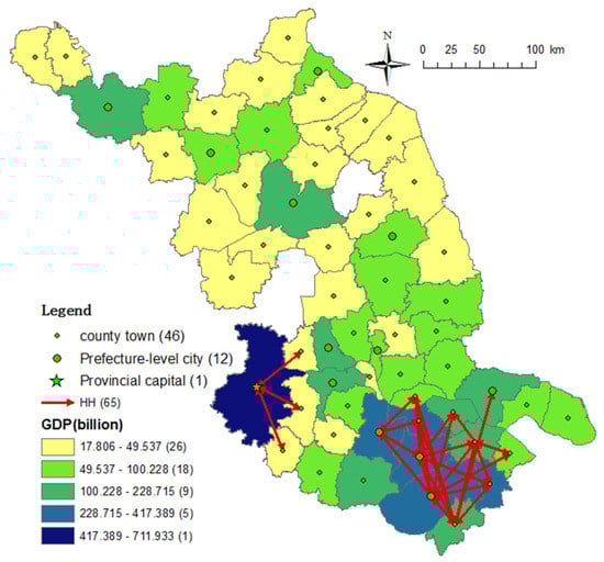
Figure 5.
Hot clusters of transport flows.
It is clear to see in Figure 5 that the hot clusters (HH) were located in two areas in the south at different spatial scales: one large scale cluster around Suzhou and one small scale cluster around Nanjing. The most southerly HH cluster, full of inter-city flows, takes advantage of active economic development (high-density urban agglomeration including Suzhou, Wuxi and Changzhou cities) and well-connected road networks [38]. The small-scale cluster around Nanjing was dominated by short-distance flows from Nanjing to surrounding counties but still within the urban region. This cluster indicates the diffusion of urban activities.
4.2. Flow-Focused Spatial Interaction Model
To explain the determinants of transport flows in the Jiangsu Province, OLS regression was used to calibrate the global model, which assumes that the process remains constant throughout the study area. To seek the optimal bandwidth, a golden section search was used to calibrate the FGWR and MFGWR models. In order to compare the parameter estimates between the two models and their statistical significance, it was necessary to visualize the parameters. A t-testing statistical graph of parameter estimates was plotted for each explanatory variable in MFGWR to investigate the spatial heterogeneity.
4.2.1. OLS
The parameter estimates for the global flow model calibrated by OLS are shown in Table 2. All parameter estimations are statistically significant at 1% as tested by the t-statistic values.
Table 2.
The parameter estimates for the global flow model calibrated by OLS.
This model gained an AICc value of 11483.257 and an adjusted pseudo of 0.626. The estimated coefficients of Tpop and GDP were 1.457 and 1.068 respectively, indicating that both Tpop and GDP were positive contributors to regional transport flow. The estimated coefficient of distance was −0.009, showing a negative contribution.
4.2.2. FGWR
Considering the varied density of flows across the study area (see Figure 2), an adaptive bandwidth strategy (Equation (13)) was chosen to calibrate each local model. Based on a golden selection process, a bandwidth of 69 (meaning 69 flows were selected as a sample for the local FGWR model of each flow) was searched to achieve the minimum AICc value of 9719.491. The bandwidth 69 out of the total number of flows, which is 3481, indicates a very strong local spatial effect. The adjusted was 0.832. Compared with the global model mentioned above, the local model performed better, indicated by the increase in adjusted (from 0.626 to 0.832) and decrease in AICc value (from 11,483.257 to 9719.491).
4.2.3. MFGWR
In MFGWR, relatively independent bandwidth optimization is performed for each explanatory variable in the model. The biggest advantage of multi-scale geographic weighting is that the optimal bandwidth for each explanatory variable can be found. Thus, as far as possible, the disadvantages caused by the common bandwidth of all the explanatory variables of the FGWR model are avoided. The bandwidths of the four explanatory variables (intercept, distance, Tpop, and GDP) were 53, 3463, 57, and 47, respectively, as shown in Table 3. One variable (distance) seemed to operate at a global scale with bandwidths implying nearly a thousand nearest neighbours. The bandwidths of intercept, Tpop and GDP were 53, 57 and 47 respectively, which indicates that these three processes vary locally.
Table 3.
Model fit statistics for OLS, FGWR and MFGWR.
4.3. Comparison between FGWR and MFGWR
As argued before, spatial dependence should be considered in the process of flow modelling. The flow-focused global Moran Indice (shown in Table 4) was used to calculate the spatial autocorrelation of (both global and local) model residuals. The fixed distance band for calculating the weight was 1.39285. The global Moran Indice was 0.08505 for OLS, 0.01154 for FGWR, and 0.00596 for MFGWR (Table 4). Compared to OLS, FGWR significantly reduced spatial autocorrelation, while MFGWR outperformed FGWR. This indicates that FGWR is more efficient than OLS in considering spatial dependence, and MFGWR is the most effective of the three.
Table 4.
Comparison of global Moran I of residual between OLS, FGWR and MFGWR.
Another strength of MFGWR over FGWR is its suitability for mapping the estimated parameters across the study area [15], which is applicable to flow modelling. MFGWR and FGWR produce a set of parameter estimations and corresponding t-statistics (Table 5). The standard deviation of the parameter estimates for each explanatory variable of MFGWR is smaller than the standard deviation of the FGWR parameter estimates. This indicates that the MFGWR parameter estimates were more clustered. It can also be seen from Table 5 that the range of parameter estimates of MFGWR was smaller and more concentrated than FGWR which indicates that the surface of the FGWR parameter estimation was not smooth enough, whereas the surface of the MFGWR parameter estimation value was more uniform and smooth. Only when the t-statistic value is large enough, the estimated parameter is meaningful and interpretable [39]. At the significance level of 5%, the t-statistic threshold value is 1.96/−1.96, although MFGWR may have a slightly varied (higher) threshold value from the traditional significance test [15]. The histograms of the t-statistic values in response to three explanatory variables (distance, Tpop and GDP) are displayed in Table 5 and Figure 6. It is clear to see a proximate normal distribution for all three for FGWR. However, the t-statistic distribution of the three parameters of MFGWR is obviously not an approximately normal distribution. This is because MFGWR spatially controls the range of influence of each explanatory variable, so the frequency distribution of t-statistics is not an approximately normal distribution. At the 5% level of FGWR, there were a total of 2970 significant parameter estimations of distance, 2416 significant parameter estimations of Tpop and 2995 significant parameter estimations of GDP. At the 5% level of MFGWR, the parameter estimates for all explanatory variables were significant, which means MFGWR is more robust.
Table 5.
Comparison of parameter estimations for FGWR and MFGWR.
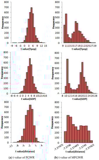
Figure 6.
Histograms of t-statistics for three parameter estimations.
4.4. Comparison of Critical Values of t Testing
The default method for the t-testing is that the 95% (α = 0.05) confidence interval corresponds to a default critical value of 1.96; the 99% (α = 0.001) confidence interval corresponds to a default critical value of 2.58. In the case of expressway transport flow, using the adjusted critical value of the t-testing method mentioned above, the 95% confidence interval for FGWR corresponded to an adjusted critical value of 3.641 and the adjusted α value was 0.00028. In MFGWR, the 95% confidence interval corresponded to an adjusted critical value of 3.6234, and the adjusted α value was 0.00029. The 95% confidence interval values for the four covariates in MFGWR corresponded to the following adjusted critical values and adjusted α values respectively; 3.6888 and 0.000229 for intercept, 3.6596 and 0.000256 for Tpop, 3.7367 and 0.000189 for GDP, 1.9606 and 0.05 for Distance (see details in Table 6).
Table 6.
Comparison of bandwidth, effective number of parameters, and critical t-values between FGWR and MFGWR.
Obviously, only the critical value of the distance explanatory variable in MFGWR was similar to the default critical value, and the other adjusted critical values were larger than the default critical value.
Table 7 shows the number of significant t-statistics after filtering the t-statistics of FGWR and MFGWR using the default critical value and the adjusted critical value. In FGWR, since the adjusted critical value was larger than the default critical value (3.641 compared with 1.96 at the 95% confidence interval), the number of significant t-statistics after filtering is significantly reduced. In MFGWR, except for the significant number of significant t-statistics for intercept, the number of significant t-statistics of the other three explanatory variables remains unchanged.
Table 7.
Number of significant t statistic values filtered by the critical values of FGWR and MFGWR.
5. Conclusions and Limitations
5.1. Conclusions and Discussion
By focusing on understanding the patterns and processes of transport flows and their socio-economic determinants, this study has provided empirical evidence of the inter-dependence between transport and economy at the regional scale (the Jiangsu province in China) by deploying an innovative analytical method of multiscale spatial analysis for flows and big data processed from georeferenced transactions at expressway toll-gates.
Methodologically, this paper reports the first empirical study of flow modelling by considering multi scales in spatial dependence and non-stationarity or heterogeneity. Based on the spatial weight of distance-band, the flow-focused global Moran Indice has been successfully used to measure the spatial autocorrelation existing in the flow data, and the results indicate a clustering pattern at the regional scale. The follow-up flow-focused local Moran Indice detected four significant clusters of flow, among which the hot clusters (high volume flows surrounded by high volume flows) help identify two areas with a high concentration of transport flow at different spatial scales. These clusters reveal the impacts of urban and economic agglomerations on regional transport.
The global spatial interaction model calibrated by OLS confirms the positive pushing effect of Tpop in the origin county and the pulling effect of GDP in the destination county. It is clear that such strong spatial interaction is influenced by growing economic development and efficient transport infrastructure in the well-known Yangtze River Delta. The positive spatial autocorrelation in the model residuals (measured by the above-mentioned flow-focused global Moran I of flows) and the two clusters at varied scales (measured by flow focused local Moran I of flows), justify the development and application of the multiscale flow-focused geographically weighted regression approach.
The MFGWR modelling results have many implications. First of all, the spatial autocorrelation in the local modelling residuals was considerably reduced, compared with that from the global model and FGWR mentioned above. This means MFGWR has largely reflected the spatial dependence present in the flow data. Secondly, the statistics of adjusted and AICc have proved that MFGWR outperforms both the global flow model and FGWR in explaining flow patterns. The spatial distributions of parameter estimations from MFGWR reflect the heterogeneous relationships between transport and socioeconomic forces across the study area. Thereby, it is argued that MFGWR has successfully considered spatial heterogeneity. Classically, the local models are run on the same spatial scale, without considering scale effects between pulling and pushing forces or spatial barriers. MFGWR relaxes this assumption by allowing different processes to operate on different spatial scales, meaning that each covariate can be modelled on different spatial scales [21]. In the case of expressway transport flow, the optimal bandwidths for distance, population and GDP were different, especially the bandwidth of distance, which being much larger, was identified as a global variable. The bandwidths between population and GDP were quite similar and smaller than that for distance, indicating a similar local process of spatial influences. Finally, in MFGWR, the critical value of t-testing for each covariate can be adjusted, which makes MFGWR more robust.
In summary, this empirical study has confirmed that MFGWR outperforms FGWR, in capturing multi-scale spatial heterogeneity and reducing spatial dependence. Specifically, MFWGR enables the explanation of varied heterogeneity with explanatory variable across the study area.
5.2. Limitations
Based on MGWR, this paper has developed a multiscale flow-focused geographically weighted regression model and used it to analyse transport flow data from the Jiangsu province in eastern China. However, this study also raises new questions for future research. Firstly, the transaction data used in this study have very a high temporal resolution. Temporal heterogeneity [40], together with spatial heterogeneity, are two sides of a coin. Both need to be integrated into an analysis of geographic mobility. The current version of MFGWR lacks the consideration of temporal dimension. A new development of multi-scale geographically and temporally weighted flow modelling will be recommended for future work. Secondly, MFGWR is powerful for mapping parameter estimation but it is hard to visualize and interpret these geographical patterns, particularly when dealing with large-scale flows. It presents a new challenge of how to intelligently represent the flow space. Lastly, the back-fitting algorithm in MFGWR has to perform a large number of iterative operations. Further work is required to improve its operating efficiency. Parallel computing may be an efficient solution.
Author Contributions
Conceptualization, J.C., H.Z. and C.J.; methodology, L.Z.; software, L.Z.; validation, L.Z., J.C., H.Z. and C.J.; formal analysis, J.C. and H.Z.; investigation, C.J.; resources, C.J.; data curation, C.J.; writing-original draft preparation, L.Z. and C.J.; writing-review and editing, J.C.; visualization, L.Z.; supervision, J.C. and H.Z.; project administration, J.C. and H.Z.
Funding
This research was funded by National Natural Science Foundation of China, grant number 41871137, 41571134, & 41571124 and the Natural Science Foundation of the Jiangsu Higher Education Institutions, grant number 16KJA170002.
Acknowledgments
The authors thank the reviewers for their helpful comments and suggestions, which led to a significant improvement on the manuscript.
Conflicts of Interest
The authors declare no conflict of interest.
References
- Castells, M. Globalisation, networking, urbanisation: Reflections on the spatial dynamics of the information age. Urban Stud. 2010, 47, 2737–2745. [Google Scholar] [CrossRef]
- Castells, M. The Information City: Information Technology, Economic Restructuring, and the Urban Regional Process; Wiley-Blackwell: New York, NY, USA, 1989. [Google Scholar]
- Uteng, T.P.; Cresswell, T. Gendered mobilities: Towards an holistic understanding. In Gendered Mobilities; Routledge: Abingdon-on-Thames, UK, 2016; pp. 15–26. [Google Scholar]
- Batty, M. The New Science of Cities; MIT Press: Cambridge, MA, USA, 2013. [Google Scholar]
- Taylor, P.; Hoyler, M.; Verbruggen, R. External urban relational process: Introducing central flow theory to complement central place theory. Urban Stud. 2010, 47, 2803–2818. [Google Scholar] [CrossRef]
- Jin, C.; Xu, J.; Lu, Y.; Huang, Z. The impact of Chinese Shanghai-Nanjing high-speed rail on regional accessibility. Geogr. Tidsskr.-Dan. J. Geogr. 2013, 113, 133–145. [Google Scholar] [CrossRef]
- Preston, J. Integrating transport with socio-economic activity: A research agenda for the new millennium. J. Transp. Geogr. 2001, 9, 13–24. [Google Scholar] [CrossRef]
- Ke, W.; Chen, W.; Yu, Z. Uncovering Spatial Structures of Regional City Networks from Expressway Traffic Flow Data: A Case Study from Jiangsu Province, China. Sustainability 2017, 9, 1541. [Google Scholar] [CrossRef]
- Yoshida, I. Relations between urban structure and transport planning in the Tokyo metropolitan area. J. Geogr. 2014, 123, 233–248. [Google Scholar] [CrossRef][Green Version]
- Marti-Henneberg, J. Challenges facing the expansion of the high-speed rail network. J. Transp. Geogr. 2015, 42, 131–133. [Google Scholar] [CrossRef]
- Dijksterhuis, A.; Bargh, J.A. The perception–behavior expressway: Automatic effects of social perception on social behavior. In Advances in Experimental Social Psychology; Academic Press: Cambridge, MA, USA, 2001; Volume 33, pp. 1–40. [Google Scholar]
- Mohl, R.A. The interstates and the cities: The U.S. department of transportation and the freeway revolt, 1966–1973. J. Policy Hist. 2008, 20, 193–226. [Google Scholar] [CrossRef]
- Liu, H.B.; Liu, Z.L. Spatial economic interaction of urban agglomeration: Gravity and intercity flow modeling & empirical study. In Proceedings of the 2008 International Conference on Management Science and Engineering 15th Annual Conference Proceedings, Long Beach, CA, USA, 10–12 September 2008; pp. 1811–1816. [Google Scholar]
- Tong, D.; Liu, T.; Li, G.; Yu, L. Empirical analysis of city contact in Zhujiang (pearl) River Delta, China. Chin. Geogr. Sci. 2014, 24, 384–392. [Google Scholar] [CrossRef]
- Fotheringham, A.S.; Brunsdon, C.; Charlton, M. Geographically Weighted Regression: The Analysis of Spatially Varying Relationships; Wiley: Chichester, UK, 2002. [Google Scholar]
- Kordi, M.; Fotheringham, A.S. Spatially Weighted Interaction Models (SWIM). Ann. Am. Assoc. Geogr. 2016, 106, 990–1012. [Google Scholar] [CrossRef]
- Zhang, L.F.; Cheng, J.; Jin, C. Spatial Interaction Modeling of OD Flow Data: Comparing Geographically Weighted Negative Binomial Regression (GWNBR) and OLS (GWOLSR). ISPRS Int. J. Geo-Inf. 2019, 8, 220. [Google Scholar] [CrossRef]
- Tao, R.; Thill, J.C. FlowAMOEBA: Identifying regions of anomalous spatial interactions. Geogr. Anal. 2019, 51, 111–130. [Google Scholar] [CrossRef]
- Cheng, J.; Forthringham, S. Multi-scale issues in cross-border comparative analysis. Geoforum 2013, 46, 138–148. [Google Scholar] [CrossRef]
- Cheng, J.; Masser, I. Modelling urban growth patterns: A multi-scale perspective. Environ. Plan. A 2003, 35, 679–704. [Google Scholar] [CrossRef]
- Fotheringham, A.S.; Yang, W.; Kang, W. Multiscale Geographically Weighted Regression (MGWR). Ann. Am. Assoc. Geogr. 2017, 107, 1247–1265. [Google Scholar] [CrossRef]
- Wolf, L.J.; Oshan, T.M.; Fotheringham, A.S. Single and Multiscale Models of Process Spatial Heterogeneity. Geogr. Anal. 2018, 50, 223–246. [Google Scholar] [CrossRef]
- Yu, H.; Fotheringham, A.S.; Li, Z.; Oshan, T.; Kang, W.; Wolf, L.J. Inference in Multiscale Geographically Weighted Regression. Geogr. Anal. 2019. [Google Scholar] [CrossRef]
- Oshan, T.; Wolf, L.J.; Yu, H.; Fotheringham, A.S.; Li, Z. On the Measurement of Bias in Geographically Weighted Regression Models. OSF. 2019. [Google Scholar] [CrossRef]
- Oshan, T.M.; Li, Z.; Kang, W.; Wolf, L.J.; Fotheringham, A.S. MGWR: A Python Implementation of Multiscale Geographically Weighted Regression for Investigating Process Spatial Heterogeneity and Scale. ISPRS Int. J. Geo-Inf. 2019, 8, 269. [Google Scholar] [CrossRef]
- Jin, C.; Cheng, J.; Xu, J.; Huang, Z. Self-driving tourism induced carbon emission flows and its determinants in well-developed regions: A case study of Jiangsu province. China J. Clean. Prod 2018, 186, 191–202. [Google Scholar] [CrossRef]
- Jiangsu Bureau of Statistics. Jiangsu Statistical Yearbook 2015; China Statistics Press: Beijing, China, 2015; Volume 55–60, p. 84.
- Cheng, J.; Young, C.; Zhang, X.; Owusu, K. Comparing inter-migration within the European Union and China: An initial exploration. Migr. Stud. 2014, 2, 340–368. [Google Scholar] [CrossRef][Green Version]
- Santeramo, F.G.; Morelli, M. Modelling tourism flows through gravity models: A quantile regression approach. Curr. Issues Tour. 2016, 19, 1077–1083. [Google Scholar] [CrossRef]
- Liu, Y.; Kang, C.; Gao, S.; Xiao, Y.; Tian, Y. Understanding intra-urban trip patterns from taxi trajectory data. J. Geogr. Syst. 2012, 14, 463–483. [Google Scholar] [CrossRef]
- Tao, R.; Thill, J.C. Spatial cluster detection in spatial flow data. Geogr. Anal. 2016, 48, 355–372. [Google Scholar] [CrossRef]
- Brunsdon, C.; Fotheringham, A.S.; Charlton, M.E. Geographically weighted regression: A method for exploring spatial nonstationarity. Geogr. Anal. 1996, 28, 281–298. [Google Scholar] [CrossRef]
- Fotheringham, A.S.; O’Kelly, M.E. Spatial Interaction Models: Formulations and Applications; Kluver Academic: Dordrecht, The Netherlands, 1989. [Google Scholar]
- Tibshirani, R. Noninformative priors for one parameter of many. Biometrika 1989, 76, 604–608. [Google Scholar] [CrossRef]
- Everitt, B.J.; Robbins, T.W. Neural systems of reinforcement for drug addiction: From actions to habits to compulsion. Nat. Neurosci. 2005, 8, 1481. [Google Scholar] [CrossRef]
- Benjamini, Y.; Yekutieli, D. The control of the false discovery rate in multiple testing under dependency. Ann. Stat. 2001, 29, 1165–1188. [Google Scholar]
- Da Silva, A.R.; Fotheringham, A.S. The multiple testing issue in geographically weighted regression. Geogr. Anal. 2016, 48, 233–247. [Google Scholar] [CrossRef]
- Wang, L.; Zhao, P. From dispersed to clustered: New trend of spatial restructuring in China’s metropolitan region of Yangtze River Delta. Habitat Int. 2018, 80, 70–80. [Google Scholar] [CrossRef]
- Byrne, D.; Ragin, C.C. The Sage Handbook of Case-Based Methods; Sage Publications: Saunders Oaks, CA, USA, 2009. [Google Scholar]
- Jin, C.; Cheng, J.; Xu, J. Using user-generated content to analyze the temporal heterogeneity of tourist mobility. J. Travel Res. 2018, 57, 779–791. [Google Scholar] [CrossRef]


© 2019 by the authors. Licensee MDPI, Basel, Switzerland. This article is an open access article distributed under the terms and conditions of the Creative Commons Attribution (CC BY) license (http://creativecommons.org/licenses/by/4.0/).