A Research on the Simultaneous Localization Method in the Process of Autonomous Underwater Vehicle Homing with Unknown Varying Measurement Error

Abstract

We propose an acoustic-based framework for automatically homing an Autonomous Underwater Vehicle (AUV) to the fixed docking station (F-DS) and mobile docking station (M-DS). The proposed framework contains a simultaneous localization method of AUV and docking station (DS) and a guidance method based on the position information. The Simultaneous localization and mapping (SLAM) algorithm is not available as the statistical characteristics of the measurement error of the observation system are unknown. To solve this problem, we propose a data pre-processing method. Firstly, the measurement error data of acoustic sensor are collected. Then, We propose a Variational Auto-Encoder (VAE) based Gaussian mixture model (GMM) for estimating the statistical characteristics of measurement error. Finally, we propose a support vector regression (SVR) algorithm to fit the non-linear relationship between the statistical characteristics of measurement error and its corresponding working distance. We adopt a guidance method based on line-of-sight (LOS) and path tracking method for homing an AUV to the fixed docking station (F-DS) and mobile docking station (M-DS). The lake experimental data are used to verify the performance of the localization with the estimated statistical characteristics of measurement error.

1. Introduction

Autonomous underwater vehicles (AUVs) play important roles in underwater missions. However, the working time is limited by on-board energy and storage capability of AUVs. The autonomous recovery of AUVs is used for recharging, data transfer, and relaunch. Docking stations can either be stationary [1,2,3,4,5,6] or mobile [7,8,9,10,11]. The process of AUV sailing from far-end to the docking station is called homing. The homing process aims at the precise physical contact between AUVs and docking stations. Physical contact can be passive or active. A common kind of passive contact is that an AUV is captured by a robotic manipulator. A common kind of active contact is that an AUV catches a cable or pole [12,13,14] with a latch or hook. The other kind of active contact is using funnel-like [15,16,17] docking stations. In this work, We address the recovery of an AUV by actively docking with a funnel-like docking station.

One of the key technologies in homing is navigation. The positions of AUV and DS should be simultaneously sensed by AUV. Three kinds of sensors are available for the position sensing of DS: (1)electromagnetic sensors, (2) acoustic sensors, and (3) optical sensors. Acoustic sensors have the longest working range, but the lowest precision. Woods Hole Oceanographic Institution (WHOI) [18,19] conducted a research on the AUV homing method based on acoustic guidance. The transceiver installed in the head of the AUV receives an acoustic signal from the beacon installed on the DS, and measures its position relative to the beacon. The absolute position of AUV is calculated indirectly as it knows the absolute position of the beacon. Electromagnetic sensors have a better precision, but much less range, about 30–50 m. Massachusetts Institute of Technology (MIT) [20] proposed the electromagnetic guidance method. In this way, the final docking accuracy can reach 20 cm. However, due to some physical factors, the effective docking range is 20–30 m. Optical sensors have the shortest range, but the highest precision. National Radiology Solutions (NRaD) [21] proposed an optical docking system, which was demonstrated to be accurate and robust for vehicle terminal guidance and provided targeting accuracy on the order of 1 centimeter under real-world conditions, even in turbid bay water. According to the characteristics of the sensors, they usually combined acoustic and optical sensors for AUV recovery. In this work, we focused on the development of acoustic-based AUV recovery algorithms since the vision guidance technology is maturing. More importantly, if the positional error of acoustic sensor is large, it may result in the inability to enter the terminal guidance phase based on vision, resulting in a failed docking.

Acoustic methods can be used at large distance. One such method for localization, is range-only localization. Range-only measurements are extensively used in many underwater homing application [22,23,24,25,26]. However, these measurements present a high-nonlinear and standard Extended Kalman Filters (EKFs) cannot cope with it. The solution to the range-only localization for homing problem using a sum of Gaussian filter is proposed in Reference [27]. The other method for localization, is range-bearing localization. In this work, the range and bearing of beacon are provided by the acoustic sensor. In other words, we can obtain the projections of distance from the transceiver to the beacon in the x and y directions of the observation coordinate system. Some SLAM algorithms for AUV have been applied to sense the position of a robot and map its surroundings simultaneously [28,29,30,31]. These algorithms are not suitable for our recovery system as the statistical characteristics of our measurement error are non-Gaussian and unknown. We adopt the improved SLAM algorithm to simultaneously sense the positions of AUV and DS.

The novel contributions of this paper include:

• We propose a method to collect the measurement error data for the observation system with the unknown statistical characteristics of measurement error.
• We propose a Variational auto-encoder based on a Gaussian mixture model to estimate the overall distribution of all measurement error data. The advantage of this method is that it can be used in both Gaussian and non-Gaussian cases.
• We adopt the support vector regression algorithm to divide the overall distribution into multiple single Gaussian distributions and their corresponding working ranges, and fit the non-linear relationships between them. It is always available when the working range of acoustic sensor exceeds the maximum working range corresponding to the measurement error data.

2. System Overview

In this section, we introduce an overview of our recovery system. We illustrate the recovery system in Figure 1. The recovery system includes a mother vessel (called AUV-I) and a sub-AUV (called AUV-$II$) for recovery. The DS was rigidly fixed to the underbelly of AUV-I. The entrance of the DS was funnel-like and was 2 m in diameter. When we need an F-DS, AUV-I remains hovering. When we need a M-DS, AUV-I moves at a constant speed in a straight line. AUV-$II$ was a torpedo-shaped vehicle that was 384 mm in diameter and 5486 mm in length. It was equipped with a Doppler velocity log (DVL), inertial measurement unit (IMU), GPS and an acoustic sensor. The acoustic senor—Evologics 32C R—was used for long-range positioning. The IMU used in our recovery system is manufactured by a Chinese scientific research institution with high precision.

We propose a data pre-processing method for SLAM with unknown measurement error. The overview of our system is shown in Figure 2.

3. Data Pre-Processing

The working medium of an acoustic sensor is sea water. The ocean is a very complex acoustic medium, whose complexity is mainly reflected in different acoustic propagation rules with the change of sea area and season. Due to the viscosity and heat conductivity of seawater, some of the sound energy is absorbed by seawater. Air bubbles, suspended particles, uneven water masses, plankton, and uneven boundaries in seawater can cause acoustic signal scattering. The above phenomenons will cause the energy loss of the signal from the source in the process of transmission. In addition, due to the non-uniform sound velocity in sea water, the sound line will be refracted, so the acoustic source signal may not reach the receiving point at a long distance. On the other hand, due to the existence of a large number of scatterers and uneven interfaces in the ocean, when the acoustic source emits sound waves, it will encounter these scatterers and generate scattered waves, which will interfere with the reception of acoustic signals. In conclusion, due to the working medium and working principle of the acoustic sensor, the measurement results of the acoustic sensor will have certain errors, and the farther the working distance is, the greater the interference will be and the greater the error will be.

Table 1. Navigation data of our recovery system.

	1	2	3	4
$\left(x_{AUV},y_{AUV}\right)$	$[800.0205,300.0763]$	$[730.6679,249.8969]$	$[680.1911,184.9589]$	$[650.2868,145.8485]$
$\left(x_{DS},y_{DS}\right)$	$[665.9183,178.3197]$	$[629.7143,123.7123]$	$[601.9309,83.1256]$	$[584.3957,58.0357]$
$Di{s}_x$	−39.9557	−10.3142	−5.6934	−3.4857
$Di{s}_y$	176.6203	161.2694	128.3054	109.6431
$Z_x$	−28.3	−1.5	−0.9	1.1
$Z_y$	160.9	151.6	120.5	101.7
$\left(x_{AUV},y_{AUV}\right)$	$[600.0220,75.7450]$	$[550.1815,7.1173]$	$[525.1551,-25.3517]$	$[500.7651,-59.2965]$
$\left(x_{DS},y_{DS}\right)$	$[555.0595,16.7112]$	$[525.5794,-26.8272]$	$[512.2178,-40.1101]$	$[498.4322,-61.5103]$
$Di{s}_x$	−2.9681	−0.6816	−2.1319	−0.6412
$Di{s}_y$	74.1472	41.9169	19.5100	3.1515
$Z_x$	0	−1.3	0	−0.4
$Z_y$	67.8	36.2	20.9	4.7

shows the navigation data of our recovery system in a sea trial.

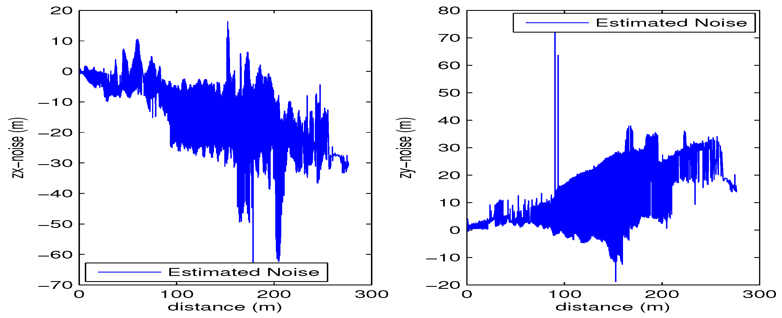
$\left(x_{AUV},y_{AUV}\right)$ and $\left(x_{DS},y_{DS}\right)$ are the positions of AUV and DS measured by IMU. These positions are true as the IMU used by our AUV has very high precision. $\left(x_{DS},y_{DS}\right)$ are the true distance between AUV and DS in X and Y direction of observation coordinate system. $Z_x$ and $Z_y$ are the measurements of acoustic sensor of AUV. We define measurement error as follows:

$$\left\{\begin{array}{l}{e}_x=Di{s}_x-z_x\\ e_y=Di{s}_y-z_y\end{array}\right.$$

(1)

The Figure 3 shows all measurement errors of this trail.

One of the premises of the SLAM algorithm is to know the statistical characteristics of the measurement error. In order to better describe the statistical characteristics of the measurement error, it is assumed that the error consists of two parts, namely, system error and random error, that is, $w=\epsilon +ϵ$. In the formula, w represents the measurement error. $\epsilon$ represents the system error. $ϵ$ is random error and follows the zero-mean Gaussian distribution. $ϵ\sim N(0,{\sigma }^2)$, where ${\sigma }^2$ is the variance of random error. In order to estimate the statistical characteristics of measurement error, firstly, the measurement error data are accumulated, then the statistical characteristics of the error are estimated by Variational auto-encoding (VAE) algorithm, and the relationship between the statistical characteristics of the measurement error and working distance is fitted by support vector regression (SVR).

3.1. Method for Accumulating Measurement Error Data

The motion model of the AUV is as follows:

$$s_k=\left\{\begin{array}{c}{x}_{k-1}+v_k·dt·cos\left({\Psi }_{k-1}+G_k\right)=x_{k-1}+d_{x,k}\\ y_{k-1}+v_k·dt·sin\left({\Psi }_{k-1}+G_k\right)=y_{k-1}+d_{y,k}\\ {\Psi }_{k-1}+G_k\end{array}\right.$$

(2)

where $v_k$ is the forward velocity of AUV at kth time. $G_k$ is the yaw angle of AUV at kth time, which constitutes the input state of AUV, that is, $u_k={\left[v_k,G_k\right]}^T$. $dt$ is the sampling interval time. The measurement coordinate system is shown in Figure 4:

The measurement model corresponding to the coordinate system shown in Figure 4 is as follows:

$$h=\left\{\begin{array}{c}\alpha =\frac{3}{2}\pi -{\Psi }_{DS}\\ z_x=-\left(x_v-x_f\right)cos\left(\alpha \right)+\left(y_v-y_f\right)sin\left(\alpha \right)\\ z_y=\left(x_v-x_f\right)sin\left(\alpha \right)+\left(y_v-y_f\right)cos\left(\alpha \right)\end{array}\right.$$

(3)

The distance between AUV and DS at kth time is calculated by the Equation (4):

$$di{s}_k=\sqrt{{(x_{v,k}-x_{f,k})}^2+{(y_{v,k}-y_{f,k})}^2}$$

(4)

Assuming that we know the initial position of AUV, first of all, $\left(x_{v,k},y_{v,k}\right)$ denotes the position of AUV at kth time. $(x_{f,k},y_{f,k})$ denotes the position of F-DS or M-DS at kth time. $(z_{x,k},z_{y,k})$ denotes the measurement of acoustic sensor at kth time. Under the premise of only using an acoustic sensor, the method 1 is used to obtain measurement error data in the process of AUV homing to F-DS:

for $k=1,\cdots$

• According to the initial position, heading and speed of AUV and Equation (2), $\left(x_{v,k},y_{v,k}\right)$ is calculated.
• According to $(z_{x,k},z_{y,k})$, $\left(x_{v,k},y_{v,k}\right)$ and Equation (3), $(x_{f,k},y_{f,k})$ is calculated.
• AUV is guided to the F-DS by line-of-sight guidance. When AUV reaches the position of F-DS, namely $x_{v,k}=x_{f,k},y_{v,k}=y_{f,k}$, end for.
• The position of F-DS at this time is true, namely $x_f=x_{f,k},y_f=y_{f,k}$.
• According to the position of AUV at $1:k$th time, $(x_f,y_f)$ and Equation (3), the true measurements at $1:k$th time, that are, $\left\{{\tilde{z}}_{x,1},\cdots ,{\tilde{z}}_{x,k},{\tilde{z}}_{y,1},\cdots ,{\tilde{z}}_{y,k}\right\}$ are calculated.
• The measurement errors at $1:k$th time are the difference between $\left\{{\tilde{z}}_{x,1},\cdots ,{\tilde{z}}_{x,k},{\tilde{z}}_{y,1},\cdots ,{\tilde{z}}_{y,k}\right\}$ and $\left\{z_{x,1},\cdots ,z_{x,k},z_{y,1},\cdots ,z_{y,k}\right\}$.
• The distances between AUV and F-DS at $1:k$th time, that is, $\left\{di{s}_1,\cdots ,di{s}_k\right\}$ are calculated.

The method 2 is used to obtain measurement error data in the process of AUV homing to M-DS:

for $k=1,\cdots$

• According to the initial position, heading and speed of AUV and Equation (2), $\left(x_{v,k},y_{v,k}\right)$ is calculated.
• According to the heading and speed of M-DS, the distances travelled by M-DS in $dt$ time, that is, $d{x}_{f,k},d{y}_{f,k}$ are calculated.
• According to $\left(z_{x,k},z_{y,k}\right)$, $\left(x_{v,k},y_{v,k}\right)$ and Equation (3), $\left(x_{f,k},y_{f,k}\right)$ is calculated.
• AUV is guided to the M-DS by line-of-sight guidance. When AUV reaches the position of M-DS, namely $x_{v,k}=x_{f,k},y_{v,k}=y_{f,k}$, end for.
• The position of M-DS at this time is true, namely $({\tilde{x}}_{f,k},{\tilde{y}}_{f,k})=(x_{f,k},y_{f,k})$. According to this position, $d{x}_{f,k},d{y}_{f,k}$ and Equation (2), the true positions of M-DS at $1:k$th time, that is, $\left\{\left({\tilde{x}}_{f,1},{\tilde{y}}_{f,1}\right),\cdots ,\left({\tilde{x}}_{f,k},{\tilde{y}}_{f,k}\right)\right\}$ are calculated.
• According to $\left\{\left(x_{1,v},y_{1,v}\right),\cdots ,\left(x_{1,k},y_{1,k}\right)\right\}$ and $\left\{\left({\tilde{x}}_{f,1},{\tilde{y}}_{f,1}\right),\cdots ,\left({\tilde{x}}_{f,k},{\tilde{y}}_{f,k}\right)\right\}$ and Equation (3), the true measurements at $1:k$th time, that is, $\left\{{\tilde{z}}_{x,1},\cdots ,{\tilde{z}}_{x,k},{\tilde{z}}_{y,1},\cdots ,{\tilde{z}}_{y,k}\right\}$ are calculated.
• The measurement errors at time $1:k$th are the difference between $\left\{{\tilde{z}}_{x,1},\cdots ,{\tilde{z}}_{x,k},{\tilde{z}}_{y,1},\cdots ,{\tilde{z}}_{y,k}\right\}$ and $\left\{z_{x,1},\cdots ,z_{x,k},z_{y,1},\cdots ,z_{y,k}\right\}$.
• The distances between AUV and M-DS at $1:k$th time, that is, $\left\{di{s}_1,\cdots ,di{s}_k\right\}$ are calculated.

To verify the effectiveness of method 1 and method 2, we use IMU to sense the positions of AUV, F-DS and M-DS, namely $\left\{\left({\overline{x}}_{v,1},{\overline{y}}_{v,1}\right),\cdots ,\left({\overline{x}}_{v,k},{\overline{y}}_{v,k}\right)\right\},\left\{\left({\overline{x}}_{f,1},{\overline{y}}_{f,1}\right),\cdots ,\left({\overline{x}}_{f,k},{\overline{y}}_{f,k}\right)\right\}$. According to Equation (3), the measurements at $1:k$th time, that is, $\left\{\left({\overline{z}}_{x,1},{\overline{z}}_{y,1}\right),\cdots ,\left({\overline{z}}_{x,k},{\overline{z}}_{y,k}\right)\right\}$ are calculated. The measurement errors at $1:k$th time are the difference between $\left\{\left({\overline{z}}_{x,1},{\overline{z}}_{y,1}\right),\cdots ,\left({\overline{z}}_{x,k},{\overline{z}}_{y,k}\right)\right\}$ and $\left\{z_{x,1},\cdots ,z_{x,k},z_{y,1},\cdots ,z_{y,k}\right\}$.

We utilize three sets of experimental data of our recovery system. Figure 5 and Figure 6 show the true and estimated measurement error data and their corresponding operating distance in AUV homing to F-DS, respectively. Figure 7 is the comparison between them. The Figure 8 and Figure 9 are the true and estimated measurement error data and their corresponding operating distance in AUV homing to M-DS, respectively. Figure 10 is the comparison between them. The comparison results show that the system error of estimated measurement error is close to that of true measurement error. Although there are some deviations between them, the estimated measurement error can reflect the statistical characteristics of measurement error when only using acoustic sensor. The methods mentioned above are not suitable for the long-distance situation, because the mileage error of AUV for long-distance is large, which results in a large gap between the estimated measurement error and the true measurement error.

3.2. Variational Auto-Encoder Based on Gaussian Mixture Model

The measurement error corresponding to each operating distance follows a single Gaussian distribution, and the measurement errors corresponding to multiple working distances follow the Gaussian mixture distribution as a whole. We adopt a variational auto-encoder based on a Gaussian mixture model to estimate the statistical characteristics of the measurement error data.

3.2.1. Variational Auto-Encoder

Variational Auto-Encoder (VAE) [32,33] is a deep generation model, which aims to build a distribution model $p_{model}$ to approximate unknown data distribution $p_{data}$. The data set $X={\left\{x_i\right\}}_{i=1}^N$ contains N independent and identically distributed discrete variables. Assuming that the variable x is generated by the latent variable z, the generating process is as follows: (1) The variable z is generated, which is denoted as $p_{\theta }\left(z\right)$; (2) The variable x is generated, which is denoted as $p_{\theta }\left(x\mid z\right)$. In addition, $q_{\varphi }\left(z\mid x\right)$ is used to approximate a posteriori probability $p_{\theta }\left(z\mid x\right)$ which is difficult to calculate. The whole process is shown in Figure 11.

The edge likelihood of X is obtained by summing the edge likelihood of each independent data. Namely:

$$log{p}_{\theta }\left(x^{\left(1\right)},\cdots ,x^{\left(N\right)}\right)=\sum _{i=1}^{N}log{p}_{\theta }\left(x^{\left(i\right)}\right)$$

(5)

Since $q_{\varphi }\left(z\mid x\right)$ approximates $p_{\theta }\left(z\mid x\right)$, then:

$$log{p}_{\theta }\left(x^{\left(i\right)}\right)=D_{KL}\left(q_{\varphi }\left(z\mid x^{\left(i\right)}\right)\Vert p_{\theta }\left(z\mid x^{\left(i\right)}\right)\right)+L\left(\theta ,\varphi ;x^{\left(i\right)}\right)$$

(6)

The first term on the right side of the equation is the Kullback-Leibler (KL) divergence of approximate from the true posterior. Since the KL divergence is non-negative, the second item on the right side of the equation is called the (variational) lower bound on the marginal likelihood of data-point i, and can be written as:

$$L\left(\theta ,\varphi ;x^{\left(i\right)}\right)=-D_{KL}\left(q_{\varphi }\left(z\mid x^{\left(i\right)}\right)\Vert p_{\theta }\left(z\right)\right)+E_{q_{\varphi }\left(z\mid x^{\left(i\right)}\right)}\left[log{p}_{\theta }\left(x^{\left(i\right)}\mid z\right)\right]$$

(7)

Let the latent variable z be the normal Gaussian distribution and $p_{\theta }\left(x\mid z\right)$ be the Gaussian distribution. So formula (3) can be written as follows:

$$L\left(\theta ,\varphi ;x^{\left(i\right)}\right)\cong \frac{1}{2}\sum _{j=1}^J\left(1+log\left({\left({\sigma }_j^{\left(i\right)}\right)}^2\right)-{\left({\mu }_j^{\left(i\right)}\right)}^2-{\left({\sigma }_j^{\left(i\right)}\right)}^2\right)+\frac{1}{L}\sum _{l=1}^{L}log{p}_{\theta }\left(x^{\left(i\right)}\mid z^{\left(i,l\right)}\right)$$

(8)

The reparameterization is $z^{\left(i,l\right)}={\mu }^{\left(i\right)}+{\sigma }^{\left(i\right)}\odot {ϵ}^{\left(l\right)}$. Where ${ϵ}^{\left(l\right)}$ is an auxiliary noise variable, and ${ϵ}^{\left(l\right)}\sim N(0,I))$. The objective of optimization is to make $log{p}_{\theta }\left(x^{\left(i\right)}\right)$ as large as possible. We use a neural network for the probabilistic encoder $q_{\varphi }\left(z\mid x\right)$ and where the parameters $\varphi$ and $\theta$ are optimized jointly with the auto-encoding variational Bayes algorithm. The variational approximation distribution can be regarded as an encoder, which maps observable variables to latent variables. The generated model can be regarded as a decoder, which maps latent variables into observable variables. The structure of VAE is shown in Figure 12.

The traditional VAE algorithm assumes that the posterior distribution $p_{\theta }\left(z\mid x\right)$ of the latent variable z satisfies a single Gaussian distribution, which is easy to cause the low-dimensional representation is too simple and cannot fit the space of the latent variable well, leading to the low accuracy of the generated model. Based on this, the Gaussian mixture model is used to fit the latent variable space.

3.2.2. Gaussian Mixture Model

The Gaussian model is a commonly used variable distribution model. The probability density function of one-dimensional Gaussian distribution is as follows:

$$f\left(x\mid \mu ,{\sigma }^2\right)=\frac{1}{\sqrt{2\pi }\sigma }exp\left(-\frac{{\left(x-\mu \right)}^2}{2{\sigma }^2}\right)$$

(9)

In the formula, x is a variable, $\mu$ and ${\sigma }^2$ are the mean and variance of Gaussian distribution, respectively.The essence of the Gaussian mixture model is to fuse several single Gaussian models to make the model more complex. The one-dimensional Gaussian mixture distribution is expressed as follow:

$$p\left(x\right)=\sum _{k=1}^K{\omega }_{k}f\left(x\mid {\mu }_k,{\sigma }_k^2\right)$$

(10)

In the formula, K is the number of single Gaussian distribution in the Gaussian mixture model. ${\omega }_k$ is the weight of the kth Gaussian distribution, and $0\le {\omega }_k\le 1$, ${\sum }_{k=1}^K{\omega }_k=1$. Theoretically, if there are enough single Gaussian models fused by the Gaussian mixture model and the weight design between them is reasonable enough, the Gaussian mixture model can fit arbitrarily distributed samples [34].

Since we cannot directly observe which distribution the data x comes from, we introduce a latent variable $z_k$ represents the probability that data x comes from the kth Gaussian distribution. Assuming that $z_k$ is independent and identically distributed, then $p\left(z\right)=p\left(z_1\right)p\left(z_2\right)\cdots p\left(z_k\right)={\prod }_{k=1}^K{\pi }_k^{z_k}$. Where $z_k\in \left\{0,1\right\},{\sum }_{k=1}^K{z}_k=1,p\left(z_k=1\right)={\pi }_k$. The probability form of conditional probability based on latent variable z is as follows:

$$p\left(x\mid z\right)=\prod _{k=1}^{K}N{\left(x\mid {\mu }_k,{\sigma }_k^2\right)}^{z_k}$$

(11)

Thus, the form of $p\left(x\right)$ is as follows:

$$p\left(x\right)=\sum _{z}p\left(z\right)p\left(x\mid z\right)=\sum _z\left(\prod _{k=1}^K{\pi }_k^{z_k}N\left(x\mid {\mu }_k,{\sigma }_k^2\right)\right)=\sum _{k=1}^K{\pi }_{k}N\left(x\mid {\mu }_k,{\sigma }_k^2\right)$$

(12)

3.2.3. Improved Variational Auto-Encoder

In this paper, the measurement error data set is used as the input of the VAE algorithm. The measurement error corresponding to each working range follows a single Gaussian distribution. Therefore, the Gaussian mixture model is used to describe the overall distribution of all measurement error data. The output of Decoder are the parameters of the Gaussian mixture model of measurement error data.

The latent variable z is assumed to have a normal Gaussian distribution in the traditional VAE algorithm. The Variational auto-encoder based on Gaussian mixtrue model (VAE-GMM) algorithm assumes that the hidden variable z is the Gaussian mixture distribution. Namely: $p_{\theta }\left(z\right)={\sum }_{i=1}^N{\alpha }_{i}N\left(0,1\right)$. Variational posterior distribution $q_{\varphi }\left(z\mid w\right)={\sum }_{i=1}^N{\pi }_{i}N\left({\mu }_{zi},{\sigma }_{zi}^2\right)$. Since the coefficients of the GMM cannot be trained and updated as trainable parameters by back propagation algorithm, the coefficients of the GMM are super-parameters, that is, ${\alpha }_i={\pi }_i=\frac{1}{N}$. Then:

$$\begin{array}{cc}\hfill & D_{KL}\left(q_{\varphi }\left(z\mid w\right)\Vert p_{\theta }\left(z\right)\right)\hfill \\ & ={\displaystyle \sum _{i=1}^N}{\pi }_i\left(log\frac{{\pi }_i}{{\alpha }_i}+D_{KL}\left(N\left({\mu }_{zi},{\sigma }_{zi}^2\right)\Vert N(0,1)\right)\right)\hfill \\ & ={\displaystyle \sum _{i=1}^N}\left(\frac{1}{N}·\left(1+log\left({\sigma }_{zi}^2\right)-{\mu }_{zi}^2-{\sigma }_{zi}^2\right)\right)\hfill \end{array}$$

(13)

$$-ln\left(q\left(w\mid z\right)\right)=\sum _{i=1}^N{\pi }_i\left(\frac{{\left(w-{\epsilon }_i\right)}^2}{2{\sigma }_{wi}^2}+\frac{1}{2}ln2\pi +\frac{1}{2}ln{\sigma }_{wi}^2\right)$$

(14)

Due to the true distribution of measurement error data $p_{data\left(w\right)}$ is unknown, we use distribution $p_{model\left(w\right)}$ to approximate it.

$$p_{model}\left(w\right)=\sum _{i=1}^N{\pi }_{i}N\left(w\mid {\epsilon }_i,{\sigma }_{wi}^2\right)$$

(15)

where ${\epsilon }_i$ and ${\sigma }_{wi}^2$ are the mean and variance of the $i^{th}$ Gaussian distribution of the Gaussian mixture model optimized by Decoder respectively, that is, $w_i={\epsilon }_i+{ϵ}_i$, and ${ϵ}_i\sim N\left(0,{\sigma }_{wi}^2\right)$ where ${\epsilon }_i$ is the system error, ${\sigma }_{wi}^2$ is the variance of random error. The coefficient of $i^{th}$ Gaussian distribution is $P(p\left(di{s}_i\right)=1)={\pi }_i$. It can be understood that when the working range of acoustic sensor is $di{s}_i$, the measurement error follows a single Gaussian distribution, that is $N\left(w\mid {\epsilon }_i,{\sigma }_{wi}^2\right)$, namely the system error is ${\epsilon }_i$, the variance of random error is ${\sigma }_{wi}^2$. The structure of VAE-GMM is shown in Figure 13. The Support Vector Regression (SVR) algorithm is used to divide the overall distribution into multiple Gaussian distributions and its corresponding working range, and fit the relationship between them.

3.3. Support Vector Regression

When support vector machine (SVM) is used for classification, its basic idea is to find an optimal classification surface to separate the two classes of samples. When support vector machine is used for regression fitting analysis, its basic idea is to find an optimal classification surface so that all training samples have the least error from the optimal classification surface [35]. Support vector regression (SVR) is also divided into linear regression and non-linear regression. This paper adopts non-linear regression. Let us consider a training set $S=\left\{\left(x_1,y_1\right),\cdots ,\left(x_l,y_l\right)|x_i\in R^n,y_j\in R,\left(i,j=1\cdots l\right)\right\}$ consists of l training samples. For the sample set S which cannot be linearly separated in the original space $R^n$, using a non-linear mapping $\Phi$ to map data S into a high-dimensional feature space H, to make $\Phi \left(S\right)$ has good linear regression characteristics in feature space H. Then linear regression is carried out in feature space H, and finally returns to the original space $R^n$. The specific implementation steps of non-linear regression are as follows:

• Looking for a kernel function $K\left(s,t\right)$, makes $K\left(x_i,x_j\right)=〈\Phi \left(x_i\right),\Phi \left(x_j\right)〉$. The commonly used kernels are radial basis function, polynomial function, spline curve function, sigmoid function and so on.
• Finding the solution of the optimization problem.

  $$\left\{\begin{array}{c}min\left\{-\frac{1}{2}{\sum }_{i,j=1}^l\left({\alpha }_i-{\alpha }_i^{\ast }\right)\left({\alpha }_j-{\alpha }_j^{\ast }\right)K\left(x_i,x_j\right)+{\sum }_{i=1}^l\left({\alpha }_i-{\alpha }_i^{\ast }\right)y_i-{\sum }_{i=1}^l\left({\alpha }_i+{\alpha }_i^{\ast }\right)\epsilon \right.\\ s.t.{\sum }_{i=1}^l\left({\alpha }_i-{\alpha }_i^{\ast }\right)=0\\ 0\le {\alpha }_i,{\alpha }_i^{\ast }\le C,i=1\cdots l\end{array}\right.$$

  (16)

  In the formula, $\epsilon$ specifies the error requirement of the regression function. The smaller $\epsilon$ is, the smaller the error of the regression function is. C is a penalty factor. The larger C is, the greater the penalty for training error greater than $\epsilon$. ${\alpha }_i$, ${\alpha }_i^{\ast }$ are the optimal solution of the equation.
• Calculation.

  $$b=\left\{\begin{array}{c}{y}_j+\epsilon -{\sum }_{i,j=1}^l\left({\alpha }_i-{\alpha }_i^{\ast }\right)K\left(x_j-x_i\right),{\alpha }_i\in \left(0,C\right)\\ y_j-\epsilon -{\sum }_{i,j=1}^l\left({\alpha }_i-{\alpha }_i^{\ast }\right)K\left(x_j-x_i\right),{\alpha }_i^{\ast }\in \left(0,C\right)\end{array}\right.$$

  (17)
• The regression function is:

  $$f\left(x\right)=\sum _{i=1}^l\left({\alpha }_i-{\alpha }_i^{\ast }\right)K\left(x_j-x\right)+b,x_i\in R^n,b\in R$$

  (18)

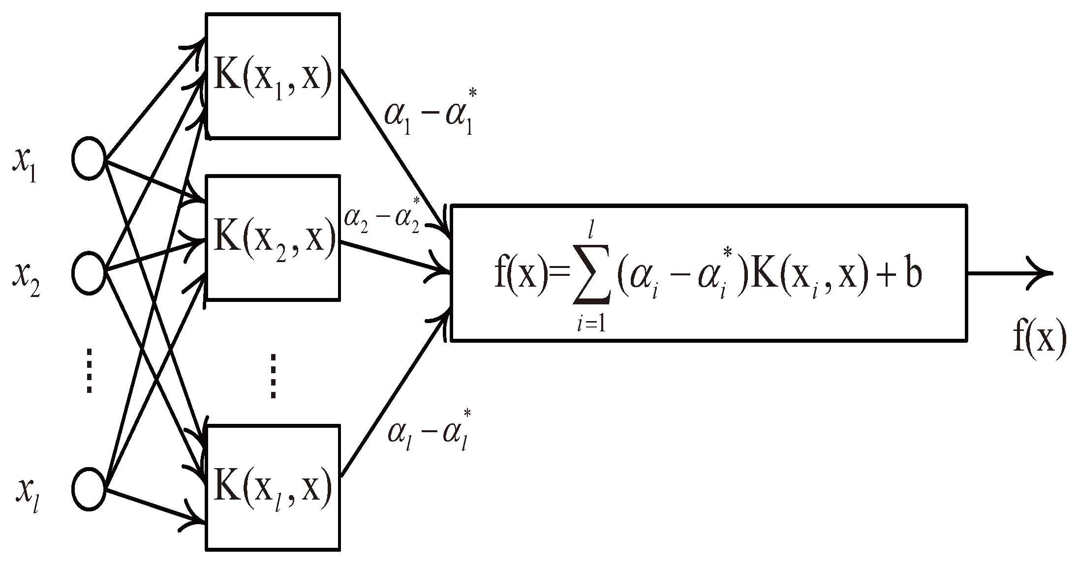
The structure of SVR is similar to that of a neural network, as shown in the Figure 14. The output is a linear combination of intermediate nodes, each of which corresponds to a support vector.

The training samples set in this paper are as follows: $S_1=\left\{\left(d_1,{\epsilon }_1\right),\cdots ,\left(d_l,{\epsilon }_l\right)\mid d_i\in R,{\epsilon }_i\in R\right\}$, $S_2=\left\{\left(d_1,{\sigma }_{w1}^2\right),\cdots ,\left(d_l,{\sigma }_{wl}^2\right)\mid d_i\in R,{\sigma }_{wi}^2\in R\right\}$. Where $d_i$ represents the working distance of an acoustic sensor. ${\epsilon }_i$ represents the system error of the acoustic sensor at this working distance. 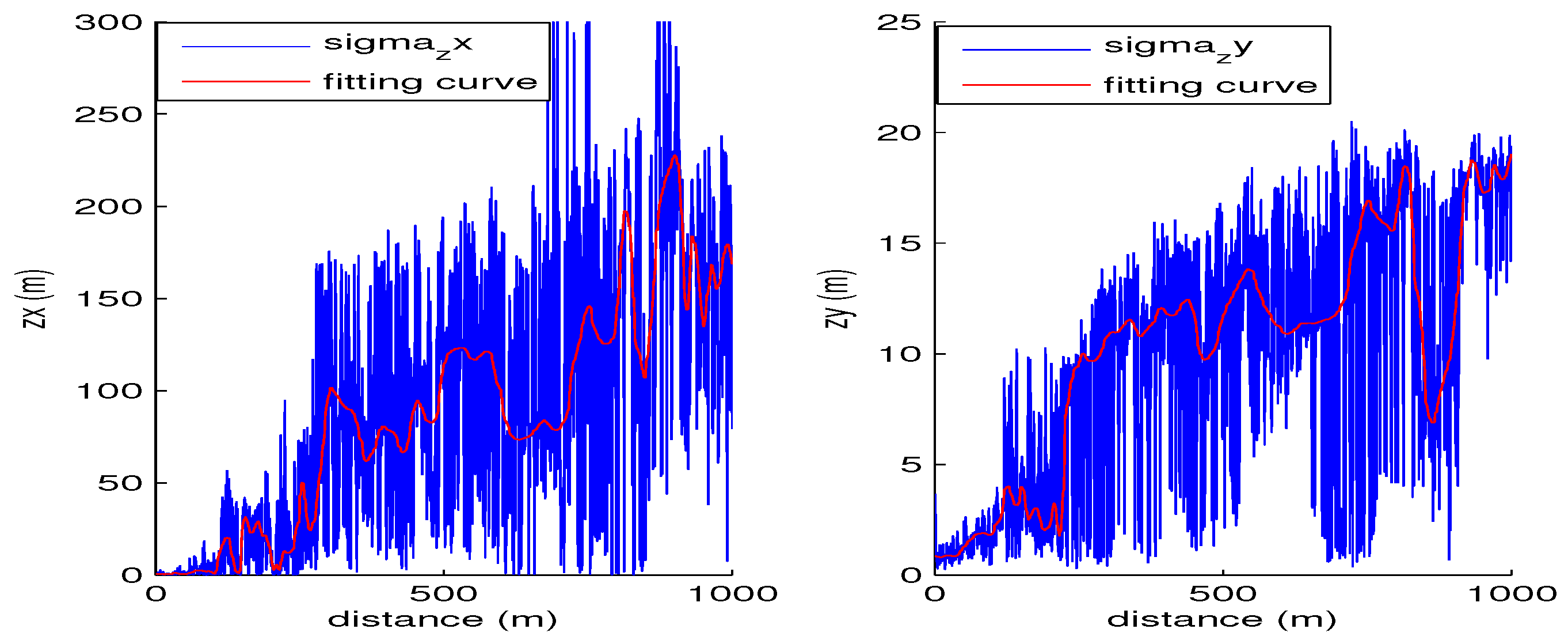${\sigma }_{wi}^2$ represents the variance of random error at this working distance. In the regression algorithm of fitting working range and system error, the radial basis function is used as the kernel function. In the regression algorithm of fitting working range and the variance of random error, the B-spline curve function is used as the kernel function. With 1000 training samples, the fitting results are shown in Figure 15 and Figure 16.

4. Simultaneous Localization of AUV and Fixed Docking Station

The states of AUV and DS are estimated simultaneously by the FastSLAM2.0 algorithm in the process of homing an AUV to the fixed DS. FastSLAM algorithm assumes that the position and attitude of AUV follow the known hypothesis distribution, and uses particle filter to estimate the posterior probability distribution of the position and attitude of AUV, where each particle represents a possible position and attitude. An EKF filter is used to estimate the posterior probability distribution of features in the environment. The joint status of SLAM is expressed as follows:

$$p\left(s^k,\Theta \mid z^k,u^k\right)=p\left(s^k\mid z^k,u^k\right)\times \prod _{m=1}^{M}p\left({\theta }_m\mid s^k,z^k,u^k\right)$$

(19)

where $s^k=s_1,s_2,\cdots s_k$ represents the state sequence of AUV, and $s_k={\left[x_k,y_k,{\Psi }_k\right]}^T$ are the position and heading angle information of AUV, respectively. ${\Theta }_m={\theta }_1,{\theta }_2,\cdots ,{\theta }_m$ are the features in the environment. $z^k=z_1,z_2,\cdots ,z_k$ represents the measurement sequence. $u^k=u_1,u_2,\cdots ,u_k$ represents the input sequence. FastSLAM algorithm includes the following four basic iteration steps:

• Sampling new trajectory particles according to the motion model of AUV.
• When new measurement is received, the EKF algorithm is used to update the state of feature in each particle.
• Calculating the importance weight of each particle.
• Resampling.

The formulas corresponding to the above algorithm are sorted out in

Table 2. FastSLAM2.0.

Step	Formula
predict	$s_k=f\left(s_{k-1},u_k\right)$
update	${\Sigma }_{sk}^{\left[m\right]}={\left[G_s^T{Q}_k^{\left[m\right]-1}{G}_s+P_k^{-1}\right]}^{-1}$
	${\mu }_{sk}^{\left[m\right]}={\Sigma }_{sk}^{\left[m\right]}{G}_s^T{Q}_k^{\left[m\right]-1}\left(z_k-{\widehat{z}}_k^{\left[m\right]}\right)+{\widehat{s}}_k^{\left[m\right]}$
	$S_c\left(k\right)=G_{\theta }{\Sigma }_{c\left(k\right)}^{\left[m\right]}\left(k-1\right)G_{\theta }^T+R\left(k\right)$
	$K_c\left(k\right)={\Sigma }_{c\left(k\right)}^{\left[m\right]}\left(k-1\right)G_{\theta }^T{S}_c{\left(k\right)}^{-1}$
	${\mu }_{c\left(k\right)}^{\left[m\right]}\left(k\right)={\mu }_{c\left(k\right)}^{\left[m\right]}\left(k-1\right)+K_c\left(z_k-{\widehat{z}}_k\right)$
	${\Sigma }_{c\left(k\right)}^{\left[m\right]}\left(k\right)=\left(I-K_c\left(k\right)H_f\right){\Sigma }_{c\left(k\right)}^{\left[m\right]}\left(k-1\right)$
	$L^{\left[m\right]}\left(k\right)=G_{s}P\left(k\right)G_s^T+G_{\theta }{\Sigma }_{c\left(k\right)}^{\left[m\right]}\left(k-1\right)G_{\theta }^T+R\left(k\right)$
	$w^{\left[m\right]}\left(k\right)={\left|2\pi L^{\left[m\right]}\left(k\right)\right|}^{-\frac{1}{2}}exp\left(-\frac{1}{2}{\left(z_k-{\widehat{z}}_k\right)}^T{L}^{\left[m\right],-1}\left(z_k-{\widehat{z}}_k\right)\right)$

:

The motion model of AUV and measurement model are shown in Equations (2) and (3).

5. Simultaneous Localization of AUV and Mobile Docking Station

Assuming that M-DS does a uniform linear motion and has good communication with AUV. The SLAM with mobile object (SLAMMO) problem based on sampling mechanism is to calculate the joint posterior probability distribution of AUV and M-DS.

$$\begin{array}{c}P\left(x_k,{\Theta }_k\mid x_{k-1},{\Theta }_{k-1},z_k,u_{x,k},u_{\Theta ,k}\right)\hfill \\ =P\left(x_k\mid x_{k-1},{\Theta }_{k-1},z_k,u_{x,k},u_{\Theta ,k}\right)·P\left({\Theta }_k\mid x_k,x_{k-1},{\Theta }_{k-1},z_k,u_{x,k},u_{\Theta ,k}\right)\hfill \end{array}$$

(20)

where $x_{k-1}$ and $x_k$ are the states of AUV at $1:k-1$ time and $1:k$ time, respectively. ${\Theta }_{k-1}$ and ${\Theta }_k$ are the states of M-DS at $1:k-1$ time and $1:k$ time, respectively. $z_k$ represents the measurement at kth time. $u_{x,k}$ represent the control input of AUV at $1:k$ time. $u_{\theta ,k}$ represent the control input of M-DS at $1:k$ time.

Firstly, the posterior probability distribution of AUV is calculated, and the proposed distribution is expanded as follows by Bayesian principle:

$$\begin{array}{c}P\left(x_k\mid x_{k-1},{\Theta }_{k-1},z_k,u_{x,k},u_{\Theta ,k}\right)\hfill \\ \stackrel{Bayes}{\propto }\eta P\left(z_k\mid x_k,x_{k-1},{\Theta }_{k-1},z_{k-1},u_{x,k},u_{\Theta ,k}\right)·P\left(x_k\mid x_{k-1},{\Theta }_{k-1},z_{k-1},u_{x,k},u_{\Theta ,k}\right)\hfill \end{array}$$

(21)

According to the motion model of AUV, the above formula is simplied to:

$$\begin{array}{c}P\left(x_k\mid x_{k-1},{\Theta }_{k-1},z_k,u_{x,k},u_{\Theta ,k}\right)\hfill \\ \stackrel{Markov}{=}\eta P\left(z_k\mid x_k,x_{k-1},{\Theta }_{k-1},z_{k-1},u_{x,k},u_{\Theta ,k}\right)·P\left(x_k\mid x_{k-1},u_{x,k}\right)\hfill \end{array}$$

(22)

Using the theory of total probability and convolution theorem, the approximate form of the proposed distribution is obtained.

$$\begin{array}{c}\hfill P\left(x_k\mid x_{k-1},{\Theta }_{k-1},z_k,u_{x,k},u_{\Theta ,k}\right)=\xi exp\left(-y_k\right)\end{array}$$

(23)

$$\begin{array}{c}\hfill S_k=R+H_{\Theta }{P}_2{H}_{\Theta }^T\end{array}$$

(24)

$$\begin{array}{c}\hfill y_k=\frac{1}{2}\left[{\left(z_k-{\widehat{z}}_k-H_x\left(x_k-{\widehat{x}}_k\right)-H_{\Theta }\left({\Theta }_k-{\widehat{\Theta }}_k\right)\right)}^T{S}_k^{-1}\left(z_k-{\widehat{z}}_k-H_x\left(x_k-{\widehat{x}}_k\right)-H_{\Theta }\left({\Theta }_k-{\widehat{\Theta }}_k\right)\right)\right]\end{array}$$

(25)

The distribution represented by the formula (23) is Gaussian, and its mean and variance are given by the minimum value and curve of the formula (25). By calculating the first order and second order of differential of $y_k$ to $x_k$, the fllowing formulas are obtained.

$$\begin{array}{c}\hfill {\Sigma }_{x,k}={\left[H_x^T{S}_k^{-1}{H}_x+P_1^{-1}\right]}^{-1}\end{array}$$

(26)

$$\begin{array}{c}\hfill {\mu }_{x,k}={\Sigma }_{x,k}{H}_x^T{S}_k^{-1}\left(z_k-{\widehat{z}}_k\right)+{\widehat{x}}_k\end{array}$$

(27)

where ${\mu }_{x,k}$ is the estimated state of AUV at kth time. ${\Sigma }_{x,k}$ is the estimated variance of AUV at kth time. Based on the sampling mechanism, the posterior probability of M-DS is calculated by the fllowing formula:

$$\begin{array}{c}P\left({\Theta }_k\mid x_k,x_{k-1},{\Theta }_{k-1},z_k,u_{x,k},u_{\Theta ,k}\right)\hfill \\ =P\left(z_k\mid {\Theta }_k,x_k,x_{k-1},{\Theta }_{k-1},z_k,u_{x,k},u_{\Theta ,k}\right)·P\left({\Theta }_k\mid x_k,x_{k-1},{\Theta }_{k-1},z_{k-1},u_{x,k},u_{\Theta ,k}\right)\hfill \\ =P\left(z_k\mid {\Theta }_k,x_k\right)·P\left({\Theta }_k\mid {\Theta }_{k-1},u_{\Theta ,k}\right)\hfill \end{array}$$

(28)

Using the same method as calculating the sate of AUV, the estimated state and variance of M-DS are as follows:

$$\begin{array}{c}\hfill {\Sigma }_{\Theta ,k}=H_{\Theta }^T{R}^{-1}{H}_{\Theta }+P_2^{-1}\end{array}$$

(29)

$$\begin{array}{c}\hfill {\mu }_{\Theta ,k}={\Sigma }_{\Theta ,k}{H}_{\Theta }^T{R}^{-1}\left(z_k-{\widehat{z}}_k\right)+{\widehat{\Theta }}_k\end{array}$$

(30)

where ${\mu }_{\Theta ,k}$ is the estimated state of M-DS. ${\Sigma }_{\Theta ,k}$ is the estimated variance of M-DS. Due to the deviation between the proposed distribution and the expected distribution, this difference is corrected by importance sampling. In the state probability distribution of AUV, the importance weight of each particle is calculated as follows:

$$\begin{array}{c}\hfill L_x=H_x{P}_1{H}_x^T+H_{\Theta }^T{R}^{-1}{H}_{\Theta }+R\end{array}$$

(31)

$$\begin{array}{c}\hfill w_x={\left|2\pi L_x\right|}^{-\frac{1}{2}}exp\left\{-\frac{1}{2}{\left(z_k-{\widehat{z}}_k\right)}^T{L}_x^{-1}\left(z_k-{\widehat{z}}_k\right)\right\}\end{array}$$

(32)

In the state probability distribution of M-DS, the importance weight of each particle is calculated as follows:

$$\begin{array}{c}\hfill L_{\Theta }=H_{\Theta x}{P}_2{H}_{\Theta }^T+R\end{array}$$

(33)

$$\begin{array}{c}\hfill w_{\Theta }={\left|2\pi L_{\Theta }\right|}^{-\frac{1}{2}}exp\left\{-\frac{1}{2}{\left(z_k-{\widehat{z}}_k\right)}^T{L}_{\Theta }^{-1}\left(z_k-{\widehat{z}}_k\right)\right\}\end{array}$$

(34)

After calculating the weight of each particle, the random resampling is used to resample. The purpose of resampling is to retain weighted particles in order to reduce the degree of particle degradation.

6. Analysis of Experimental Data

Our recovery system was tested on a lake at the xinanjiang experimental field of the institute of acoustics, Chines Academy of Sciences in December 2018. AUV sensed the position of DS by using the ultra short baseline (USBL) system and camera. The intersection of the estension line of AUV initial heading and the center of DS is the initial target point. AUV reached the target point by line-of-sight (LOS) guidance, and tracked the center line of DS. More detailed descriptions are given in Reference [36]. The experimental results are shown in Figure 17.

We use these experimental data to verify the effectiveness of the proposed algorithm. Firstly, the method 1 and method 2 are applied to collect the measurement error data of acoustic sensor. Then the VAE-GMM algorithm is applied to estimate the overall distribution of measurement error data. Finally, the SVR algorithm is used to fit the relationship between the ststistical characteristics of measurement error data and its coressponding working distance. After data pre-processing, SLAM algorithm is applied to estimate the positions of AUV and DS. The actual measurement error in the experiment and the corresponding to estimated statistical characteristics are partly shown in

Table 3. Actual measurement error and estimated statistical characteristics.

	1	2	3	4
actual error(x)	−26.0954	−20.3664	−15.4389	−15.8233
estimated mean(x)	−20.4985	−19.3341	−18.0703	−11.6306
estimated variance(x)	52.5201	65.73	68.5750	34.4198
actual error(y)	20.8992	16.0174	14.7687	9.1035
estimated mean(y)	16.2934	15.9007	15.0819	10.1747
estimated variance(y)	9.5113	12.0081	12.3802	14.8358
actual error(x)	−6.9282	−4.1194	−1.1224	0.5263
estimated mean(x)	−3.9893	−3.8044	−2.6581	0.0927
estimated variance(x)	5.9733	2.5934	0.9619	0.4035
actual error(y)	1.4114	1.5264	0.0763	−0.9784
estimated mean(y)	2.8238	2.6493	2.0045	0.5360
estimated variance(y)	3.4287	3.4820	1.2557	0.9381

. The data analysis results are shown in Figure 18, Figure 19, Figure 20 and Figure 21.

Figure 18 and Figure 20 show the deviation between the estimated position and true position of AUV sensed by IMU. We can know that the position of AUV estimated by SLAM algorithm is close to the position sensed by IMU. It is applicable if without IMU. In Figure 19 and Figure 21, the blue line shows the deviation between the position of DS estimated by SLAM and true position of DS sensed by IMU. The red line shows the deviation between the positon of DS directly estimated by the measurement of sensor and true position. We can know that the localization precision of the SLAM algorithm is higher than that of the original data.

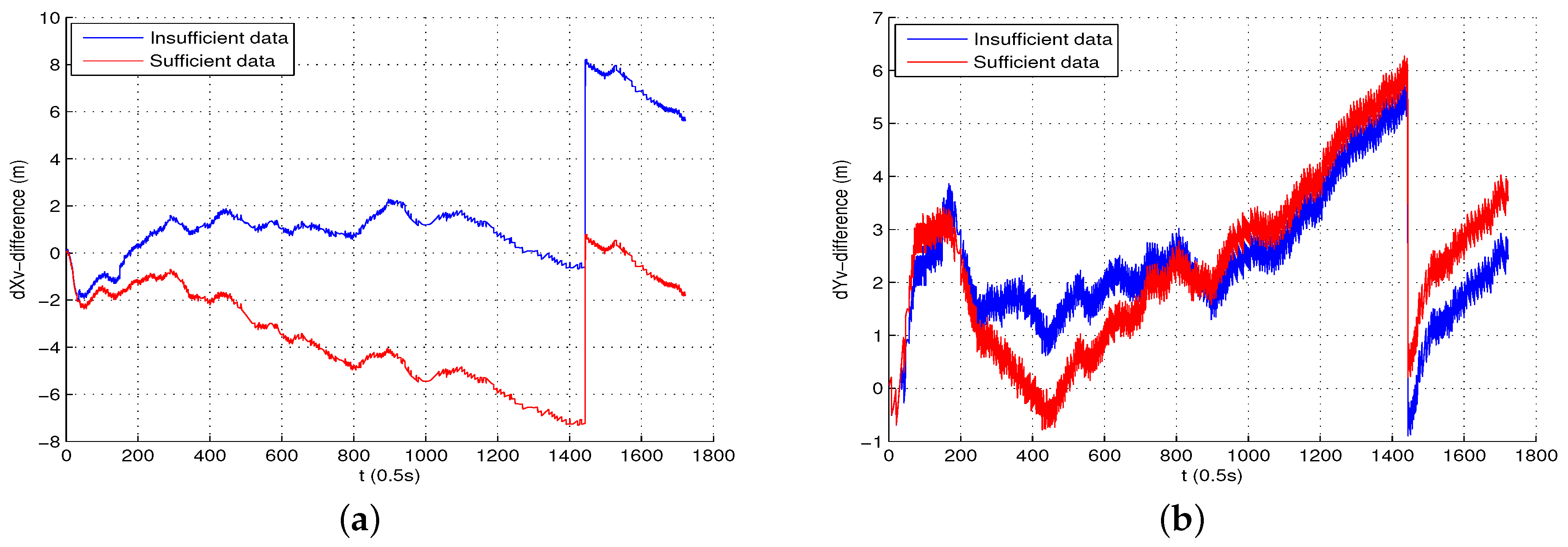
When the initial distance between AUV and DS is larger than the maximum operating distance corresponding to measurement error data, the above method can still be used. This is because the SVR method has the ability of prediction after training. In the experiment of AUV homing to the M-DS mentioned above, the initial distance between AUV and M-DS was about 207 m. Assuming that we only use measurement error data with the maximum working distance less than 150 m, the experimental data analysis results are as follows:

In Figure 22, the blue line and red line respectively show the deviation between the estimated position and the true position of AUV sensed by IMU with the the maximum working range corresponding to measurement error data less than 150 m and less than 250 m. In the Figure 23, the blue line and red line respectively show the the deviation between the estimated position and true position of M-DS sensed by IMU with the maximum working range corresponding to the measurement error data less than 150 m and less than 250 m. The black line shows the position of M-DS directly estimated by the measurement of the sensor. We can know that the positioning accuracy of the SLAM algorithm with the maximum working range corresponding to measurement error data less than 150 m is lower than that with the maximum working range corresponding to measurement error data less than 250 m, but higher than that of the original algorithm. So even if the initial distance between AUV and DS exceeds the maximum working distance corresponding to the measurement error data, the algorithm proposed in this paper is still effective.

7. Conclusions

We propose a data pre-processing method for SLAM with unknown measurement error. The measurement error data collected by method 1 and method 2 can reflect the statistical characeristics of the measurement error of an acoustic sensor. The measurement error corresponding to each working range follows a single Gaussian distribution, and the measurement errors corresponding to multiple working distances follow the Gaussian mixture distribution as a whole. The overall distribution of measurement error data is non-Gaussian, and its statistical characeristics can be estimated by a VAE-GMM algorithm. The SVR algorithm is applied to divide the overall distribution into multiple single Gaussian distributions and their corresponding working range, and fit the relationships between them. After data pre-processing, the SLAM algorithm is applied to estimate the positions of AUV and F-DS and M-DS. The analysis of experimental data shows that the position estimated by the SLAM algorithm is closer to the true position than that directly estimated by the sensor measurement.