Abstract
In this study, a rotor-bearing-runner system (RBRS) considering multiple nonlinear factors is established, and the complex nonlinear dynamic behavior of the coupling system is studied. The effects of excitation current, radial stiffness, and friction coefficient on dynamic characteristics are analyzed by numerical simulation. The research results show that the dynamic properties of the coupling system caused by different nonlinear factors are interactional. With the changes of different parameters, the RBRS presents multiple motion states, including periodic-n, quasi-periodic, and chaotic motion. The increase of the excitation current Ij has a certain inhibitory effect on the response amplitude of the system and makes the motion state of the system more complex, the chaotic motion wider, and the jump discontinuity enhanced. With the increase of radial stiffness kr, the motion complexity of the coupling system increases, the chaotic region increases, the response amplitude increases, and the vibration intensity increases. With the increase of the friction coefficient μ, the chaotic region increases first and decreases, the different motions alternate frequently, and the response amplitude gradually increases. This study can not only help to understand the dynamic characteristics of RBRS, but also help the stable operation of the generator set.
1. Introduction
A large-scale rotating generator set is a complex system involving many factors, such as mechanical and electromagnetic. The vibration failure during its operation seriously threatens the safe and stable operation of large rotating machinery. The unbalanced magnetic pull force of the rotor–stator and the rubbing of the bearing–shaft system are two important vibration fault sources of the generator set. In order to improve the vibration characteristics of the system, it is very important to establish a precise dynamic model and analyze the dynamic characteristics of the generator set. Researchers conducted a large number of analytical studies on this. Ma et al. [1] and Wen [2] gave a general introduction to the nonlinear vibration system of rotating machinery such as hydraulic turbines. Chu et al. [3] designed a rotor system test bench that can simulate rotor–stator friction and analyzed the harmonic components under different conditions. Patel et al. [4] discussed the torsional and bending vibrations of the rotor system due to friction and cracking. In Cao et al. [5]’s paper, nonlinear dynamics of the fractionally damped rub-impact rotor system are investigated. The rubbing forces consist of a radial elastic force and a tangential Coulomb friction force. The influence of speed, damping coefficient, and eccentricity is discussed. Focusing on the local rubbing problem of the generator rotor, Huang et al. [6] established a dynamic model of rotor misalignment and frictional rubbing coupling, and analyzed the dynamic response of the system. Ma et al. [7] studied the vibration characteristics of double disc rotor system when a disc and an elastic rod are rubbed, and compared it with experimental results. Considered the rubbing force, Khanlo et al. [8] studied the influence of bending-torsional coupling on the nonlinear dynamic behavior of the shaft–disc system. Jacquet-Richardet et al. [9] reviewed the numerical analysis and experimental analysis of the rotor–stator contact problem; Lu et al. [10] established a rotor dynamics model considering radial rubbing, and analyzed the dynamic characteristics of frictionless, local friction, and full-cycle friction. Ma et al. [11] studied the dynamic characteristics of rotor–stator rubbing based on contact dynamics theory; Xiang et al. [12] established a nonlinear model to study the dynamic behaviors of a rotor-bearing system under the interaction of rubbing, crack, and oil film forces. Ma et al. [13,14] studied the vibration response characteristics of dynamic and static structures rubbing. Mokhtar et al. [15] studied the nonlinear effects of system parameters on the rotor system during friction. Yang et al. [16] considered the failures of rotor imbalance and multi-point positioning friction collision, and established the dynamic model of the double-disc rotor system by using finite element theory, in which the Lankarani–Nikravesh model and the Coulomb model have been used to simulate the impact force and the frictional force. Yang et al. [17] proposed an impact force model to analyze the dynamic characteristics of a rubbing rotor system with a surface coating. Yang et al. [18] considered the unbalanced magnetic pull force of large induction motors due to rotor eccentricity and phase imbalance, and discussed methods for analyzing the instability of large induction motors. In Gustavsson et al. [19]’s paper, the influence of nonlinear magnetic pull was studied for a generator where the generator spider hub does not coincide with the center of the generator rim; Perers et al. [20] studied the mechanism of unbalanced magnetic pull generated by a synchronous generator with static eccentricity, and discussed the influence of iron saturation on the magnitude of magnetic pull. Lundström et al. [21] analyzed the influence of the rotor and stator shape deviation on the dynamic characteristics of the generator, and proved the importance of the unbalanced magnetic pull nonlinear influence; Calleecharan et al. [22] proposed a rotor model considering radial and tangential unbalanced magnetic pull forces; Xu et al. [23] studied the effect of UMP on radial vibration of hydroelectric generators, and compared and analyzed the simulation results and the field experimental data; Zeng et al. [24] established the hydro turbine generating sets dynamics model by using the unbalanced magnetic pull force acting on the generator and the unbalanced force acting on the rotor as the input excitation of the hydro turbine generating sets system; Xu et al. [25] established a hydro-generator dynamics model considering the nonlinear unbalanced magnetic pull force and the linear water unbalance force; Xu et al. [26] studied the response characteristics of unbalanced magnetic pull rotor system considering both static and dynamic eccentricity. Xiang et al. [27] analyzed the influence of unbalanced magnetic pull on the nonlinear dynamic characteristics of permanent magnet synchronous motors rotor system; Li et al. [28] established a two-dimensional hydroelectric generator electromagnetic model, using the finite element method to study the characteristics of the electromagnetic flux and electromagnetic force; Yan et al. [29] analyzed the influence of excitation current on the nonlinear dynamic behaviors of the generator. It should be noted that in all of the above research, most of them only consider one nonlinearity factor. In fact, in the vibration faults of the generator set, the multiple vibration sources are not isolated from each other, but the vibrations caused by different nonlinear factors interact with each other. Therefore, the generator set needs to be studied as a highly nonlinear coupled dynamic system. In this paper, the complex nonlinear dynamic behavior of coupled systems is studied; the influences of the excitation current, radial stiffness, and friction coefficient on the dynamic characteristics was analyzed by numerical simulation, and discussed in detail through Bifurcation diagram, 3-D frequency spectrum, waveform, frequency, axis orbit, and Poincaré map.
This article consists of four parts. In Section 2, the dynamic equation of a rotor-bearing-runner system (RBRS) is developed, meanwhile, the nonlinearity of electromagnetic force of the rotor and the nonlinearity of rubbing force of the combination bearing are considered; in Section 3, the dynamic behavior of RBRS is analyzed, and the influence of different system parameters on nonlinear systems is discussed through Bifurcation diagram, 3-D frequency spectrum, etc. Finally, some conclusions are drawn in Section 4.
2. The Dynamic Model of the RBRS
In order to study the dynamic behavior of RBRS effectively, the finite element model of double rotor-bearing system of hydraulic turbine is modeled and simplified as four lumped mass points according to the structural characteristics of the system. The rotor and the runner are located at node 1 and node 4, respectively, and the combination bearing and turbine guide bearing are located at node 2 and node 3, respectively. The schematic diagram of RBRS is shown in Figure 1. The rotation center coordinates of the turbine rotor and the runner are O1(x1, y1) and O4(x4, y4), and the centroid coordinates of the rotor and the runner are G1(xg1, yg1) and G4(xg4, yg4).
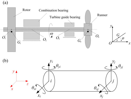
Figure 1.
(a) Schematic diagram of rotor-bearing-runner system; (b) Schematic of lumped mass point and its coordinate system.
The dynamic equation of RBRS with 16 degrees of freedom can be deduced as follows:
where M, C, G, K, q are mass matrix, damping matrix, gyroscopic matrix, stiffness matrix, and displacement vector of RBRS, respectively.
where xi, yi (i = 1,2,3,4) and θxi, θyi (i = 1,2,3,4) are the displacements of the rotor, combination bearing, turbine guide bearing, and runner in x and y directions and angles of orientation associated with the x and y axes, respectively.
Suppose that RBRS is composed of an elastic shaft element and the generalized coordinates of the shaft element are the displacements of nodes at both ends. The rotor system in this study only considers bending deformation and torsional deformation in horizontal and vertical directions, ignoring axial deformation.
where MsT, MsR,Gs (Gs = ωJs), and Ks represent moving inertia matrix of the unit, rotational inertia matrix of the unit, rotation matrix of the unit, and stiffness matrix of the unit, respectively. μ, l, and EI are the quality of the unit length, the length of the unit, and bending stiffness.

 where kz2x, kz3x, kz2y, and kz3y are the stiffness of the combination bearing and turbine guide bearing in x and y directions, respectively.
The total damping matrix (Rayleigh damping form is applied to determine the viscous part) can be obtained by the following formula [30]:
where ω1 and ω2 are the first and second natural frequencies of the system, respectively. ξ1 and ξ2 are the first and second modal damping ratios, respectively.
where cz2x, cz3x, cz2y, and cz3y are the damping of the combination bearing and turbine guide bearing in x and y directions, respectively.
where m1ρ1 and m4ρ4 denote eccentricity of unbalance mass of the generator rotor and the turbine runner.
where Fex and Fey are nonlinear electromagnetic force of the rotor in x and y directions. Nonlinear electromagnetic force can be expressed as:
where kn, ε and θr represent electromagnetic stiffness, relative eccentric, and rotation angle of the rotor. α and δ0 are variation coefficient of the electromagnetic stiffness and average air gap length. The functions kn, ε, and θr are respectively given in Equations (20)–(22):
where μ0, r, L, Kj, and Ij are permeability of vacuum, rotor radius, rotor height, coefficient of air gap fundamental wave magnetomotive force, and excitation current of the generator, respectively.
where Fwx and Fwy are the hydraulic force of the runner in x and y directions. Hydraulic force can be expressed as:
where Kw is coefficient of the hydraulic force.
where Frx and Fry are nonlinear rubbing force of the combination bearing in x and y directions. Nonlinear rubbing force can be expressed as:
where r represents vibration amplitude of the rotor. kr, δ, and f are radial stiffness of the stator, gap, and friction coefficient of rubbing. Where the functions r is given in Equation (27):
where ξ is the relative position of rotor centroid and stator centroid.
3. Nonlinear Dynamic Analysis of the RBRS
In the previous section, the dynamics model of the rotor-bearing-runner system (RBRS) is introduced and the system dynamics equation is obtained. In this section, the influence of different system parameters on nonlinear systems under the coupling of mechanical unbalance force, nonlinear magnetic pull force, hydraulic unbalance force, and nonlinear rubbing force is studied, through Bifurcation diagram, 3-D frequency spectrum, Waveform, Frequency, Axis orbit, and Poincaré map. The parameters for the coupling system are presented in Table 1. In addition, the detailed simulation condition schematic is displayed in Figure 2.

Table 1.
Model parameters of RBRS.
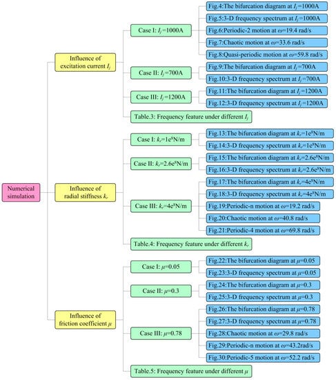
Figure 2.
Simulation condition schematic.
3.1. Model Verification
In order to verify the correctness of the non-linear dynamic model built in this paper, the accuracy of the model was verified by comparing it with the models built in the existing literature. In simulation, the parameters given in Table 1 were used in both models. As shown in Figure 3, the three-dimensional spectrum of the model in the Y direction of the rotor is given. Figure 3a is the three-dimensional spectrum of the model in reference [31]. Figure 3b is the calculation result of the model established in this paper. By comparison, it can be found that when the rotating speed is small, the frequency components of the two models are mainly one times frequency conversion fn1, and no rubbing occurs in the shafting. With the increase of rotational speed, the main components of Figure 3a are the frequency multiplication components fn1, 2fn1, 3fn1, and the frequency demultiplication component is not obvious. In addition, the amplitude of one times frequency conversion fn1 shows a fluctuating growth, while the amplitude of other frequency multiplication components increases first and then decreases. In Figure 3b, besides the frequency conversion and frequency multiplication components, there are also obvious frequency demultiplication components, such as fn1/2, 3fn1/2, 5fn1/2, 7fn1/2, etc. The amplitude of each frequency component varies nonlinearly, and at a certain speed, there is an obvious continuous spectrum component in the three-dimensional spectrum. At this time, the system is in a chaotic state, but not in Figure 3a. When the speed reaches 71 rad/s, there are only obvious fn1 and 2fn1 components in Figure 3a. Besides frequency multiplication components, Figure 3b has more obvious frequency demultiplication components.
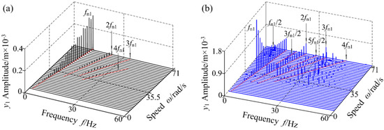
Figure 3.
(a) Adapted from reference [31]; (b) Model in this paper.
In order to compare the frequency components of the two models more clearly, Table 2 gives the comparison of frequency characteristics in three-dimensional spectrum. By comparing Figure 3 with Table 2, it can be seen that the model established in this paper takes into account the electromagnetic-rubbing coupling, non-linear electromagnetic force, hydraulic unbalance force, and other factors, which can better reflect the non-linear vibration characteristics of multi-physical field coupling.
Table 2.
Comparison of the frequency characteristics.
3.2. Influence of Excitation Current on Dynamic Characteristics of RBRS at Variable Speed
Nonlinear electromagnetic force has an important influence on the inherent characteristics and dynamic response of RBRS, which is one of the important reasons for the nonlinear characteristics of RBRS. In order to study the influence of different excitation currents of the generator Ij on the dynamic characteristics of RBRS, Figure 4 and Figure 5, respectively, give the bifurcation diagram and 3-D frequency spectrum of RBRS with rotational speed ω (ω = 7.0~71 rad/s) as control parameter at Ij = 1000 A.
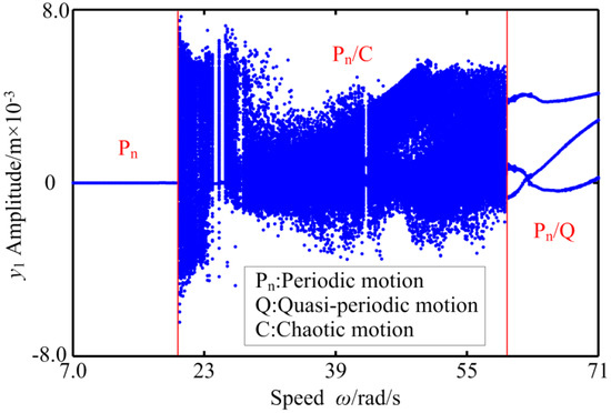
Figure 4.
The bifurcation diagram of RBRS at Ij = 1000 A.
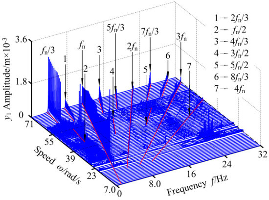
Figure 5.
3-D frequency spectrum of RBRS at Ij = 1000 A.
When the rotational speed is small, the motion state of RBRS is periodic motion, and the response amplitude is relatively stable. At the same time, the frequency component is not very obvious, mainly based on one times the frequency conversion fn. Figure 6 shows the characteristics of periodic motion at ω = 19.4 rad/s, through waveform, frequency, axis orbit, and Poincaré map. With the increase of the rotational speed, the system passes through saddle-node bifurcation at ω = 20 rad/s and enters chaotic motion. In the range of ω ∈ [20.0,59.8] rad/s, the system mainly exhibits chaotic motion, except for a few points where the vibration system presents periodic-n motion at ω = 24.4 rad/s, ω = 24.6 rad/s, ω = 42.6 rad/s, and ω = 42.8 rad/s, and has different bifurcations such as saddle-node bifurcation, period-doubling bifurcation, inverse period-doubling bifurcation; in the three-dimensional spectrum, the continuous and discrete spectral components alternate and the amplitude changes nonlinearly. The vibration responses of the RBRS at ω = 33.6 rad/s are given in Figure 7. It can be seen from the figure that the amplitude of the system vibration response increases and changes aperiodically; in the frequency domain, besides the frequency conversion and frequency multiplication components, the continuous frequency components also appear, and the axis orbit of the system is disorderedly. On the corresponding Poincaré map, the attractors are irregular discrete points, and the system exhibits chaotic motion. With the speed increasing further, when ω = 59.6 rad/s, the system moves from a short quasi-periodic motion to a stable periodic motion via the Hopf bifurcation; except for the frequency multiplication components (fn, 2fn, 3fn,...) in the 3-D frequency spectrum, there are also frequency demultiplication components (fn/3, 2fn/3, 4fn/3, 5fn/3,...), in which fn/3 is the main frequency component, and the amplitude gradually increases and is significantly larger than other frequency components. The vibration responses of the RBRS at ω = 59.8 rad/s are displayed in Figure 8. As can be seen from the figure, the coupling system is quasi-periodic motion. The main frequency components are fn, 2fn, and 3fn. Meanwhile, the attractors form a closed circle in the Poincaré map.
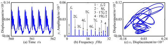
Figure 6.
Periodic-2 motion of RBRS at ω = 19.4 rad/s: (a) Waveform, (b) Frequency, and (c) Axis orbit and Poincaré map.
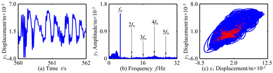
Figure 7.
Chaotic motion of RBRS at ω = 33.6 rad/s: (a) Waveform, (b) Frequency, and (c) Axis orbit and Poincaré map.
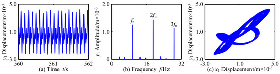
Figure 8.
Quasi-periodic motion of RBRS at ω = 59.8 rad/s: (a) Waveform, (b) Frequency, and (c) Axis orbit and Poincaré map.
In order to further comprehensively study the effects of different excitation current of the generator Ij on RBRS, Figure 9, Figure 10, Figure 11 and Figure 12, respectively, give the bifurcation diagram and 3-D frequency spectrum of RBRS at Ij = 700 A and Ij = 1200 A. By comparing the bifurcation diagrams and the 3-D frequency spectrum, it can be seen that the system shows different vibration forms and different bifurcation paths under various excitation currents. When the excitation current of the generator Ij is small, the dynamic behavior of the system is relatively simple. When ω < 20.2 rad/s, the vibration system behaves as a periodic motion, and the frequency components is not only the frequency conversion fn, but also the unobvious frequency multiplication component. As the rotational speed increases, the system transits from short-term periodic motion, chaotic motion, and quasi-periodic motion to periodic motion, successively undergoing saddle-node bifurcation, period-doubling bifurcation, inverse period-doubling bifurcation, and Hopf bifurcation. Frequency multiplication is the main frequency component in the 3-D frequency spectrum, and the peak value appears at 7fn when ω = 21.0 rad/s. When the rotational speed increases to ω = 54.8 rad/s, the system enters the chaotic motion and transits to stable periodic motion through the addle-node bifurcation, and the amplitude of response at ω = 68.0 rad/s appears obvious jumping discontinuity. Comparing Figure 4 and Figure 5, Figure 9 and Figure 10, and Figure 11 and Figure 12 shows that the dynamic behavior of the system is more complicated, and the discontinuous jump is obviously increased. As the rotational speed increases, the chaotic region becomes wider. In the range of ω ∈ [20.0,22.4] rad/s, except for the stable period-doubling motion in a small region, the system is of continuous chaotic motion or intermittency chaos motion. When ω = 29.0 rad/s, the system enters the chaotic motion through the saddle-node bifurcation, and in the range of ω > 28.8 rad/s, the vibration system exhibits strong nonlinear characteristics of periodic motion and chaotic motion frequently alternating. With the increase of the rotational speed, different bifurcation paths, such as saddle-node bifurcation, period-doubling bifurcation, and inverse period-doubling bifurcation appear in the system. The corresponding vibration amplitude increases first, then decreases and then increases nonlinearly. In order to specify the main frequency components of the system under different excitation currents of the generator Ij, the main frequency components (where fn is the frequency conversion) in different speed ranges are listed in Table 3.
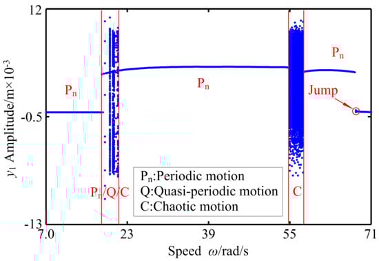
Figure 9.
The bifurcation diagram of RBRS at Ij = 700 A.
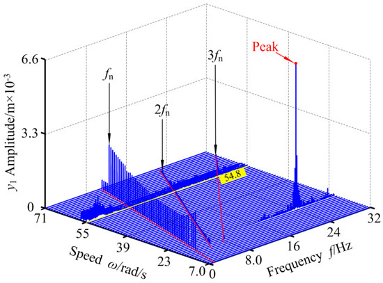
Figure 10.
3-D frequency spectrum of RBRS at Ij = 700 A.
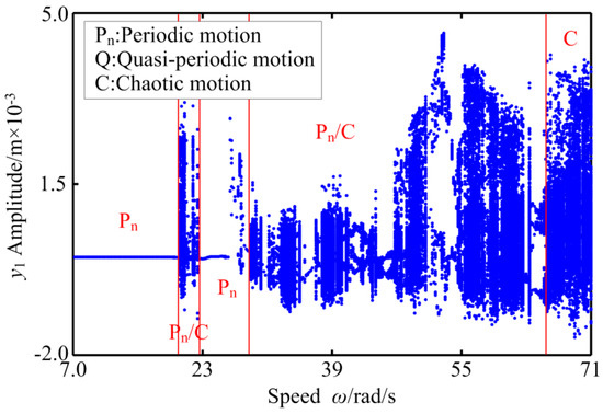
Figure 11.
The bifurcation diagram of RBRS at Ij = 1200 A.
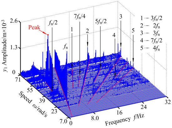
Figure 12.
3-D frequency spectrum of RBRS at Ij = 1200 A.
Table 3.
Frequency feature of RBRS under different excitation current.
Through comparison, it can be seen that the increase of the excitation current has a certain inhibitory effect on the response amplitude of the system, but it has no inhibitory effect on the motion state, which makes the motion state of the system more complex, the chaotic motion widens relatively, and the jump discontinuity is enhanced. At higher rotational speeds, the number of high-order bifurcation increases with the increase of excitation current. Therefore, it is necessary to control the excitation current within a certain range in order to enable the vibration system to operate stably.
3.3. Effect of Radical Stiffness on Dynamic Characteristics of RBRS at Variable Speed
The nonlinear radial stiffness (kr) has an important influence on the stable operation and dynamic characteristics of RBRS. In order to study the dynamic response characteristics of the coupling system with nonlinear rubbing forces at different speeds, Figure 13, Figure 14, Figure 15, Figure 16, Figure 17 and Figure 18 give the bifurcation diagram and 3-D frequency spectrum of RBRS with different radial stiffness (kr = 1 × 10⁸ N/m, kr = 2.6 × 10⁸ N/m, and kr = 4 × 10⁸ N/m). All other parameters are fixed.
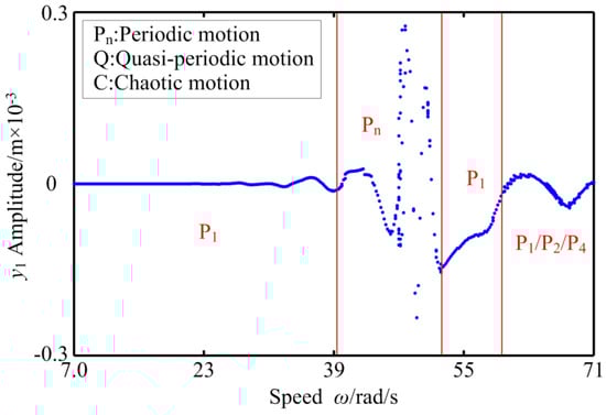
Figure 13.
The bifurcation diagram of RBRS at kr = 1 × 10⁸ N/m.
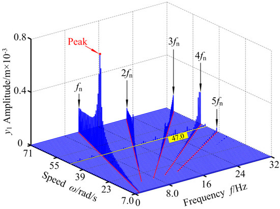
Figure 14.
3-D frequency spectrum of RBRS at kr = 1 × 10⁸ N/m.
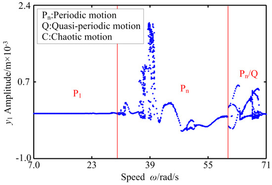
Figure 15.
The bifurcation diagram of RBRS at kr = 2.6 × 10⁸ N/m.
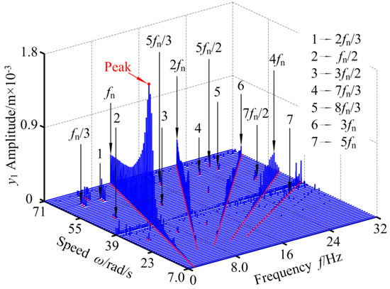
Figure 16.
3-D frequency spectrum of RBRS at kr = 2.6 × 10⁸ N/m.
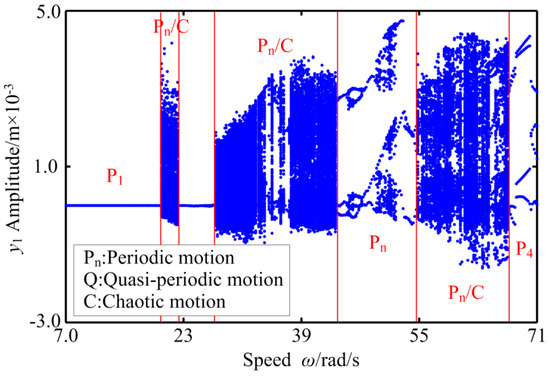
Figure 17.
The bifurcation diagram of RBRS at kr = 4 × 10⁸ N/m.
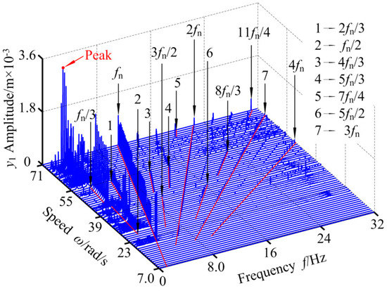
Figure 18.
3-D frequency spectrum of RBRS at kr = 4 × 10⁸ N/m.
It can be seen from Figure 13 and Figure 14 that when the radial stiffness is small, the coupling system behaves as period 1 and a double-cycle motion, and only the bifurcation path of the period-doubling bifurcation and the inverse period-doubling bifurcation appears, and discontinuous jumps occur in the range of ω ∈ [39.6,52.2] rad/s. In the three-dimensional spectrum, when the rotational speed is small, the frequency components are relatively simple, mainly the frequency multiplication components (fn, 2fn, 3fn,...). With the gradual increase of the rotational speed, besides the frequency multiplication component, the coupling system has unobvious frequency demultiplication components (fn/2, fn/3, fn/4,...) and the frequency demultiplication components alternately appear. The amplitude of the main frequency components increases first and then decreases nonlinearly (when ω = 58.0 rad/s, the c amplitude peak appears at fn). When the radial stiffness increases to kr = 2.6 × 10⁸ N/m, it can be found that the period doubling region widens, the period-doubling bifurcation and the inverse period-doubling bifurcation alternate frequently, and obvious frequency demultiplication components appear, and the transient quasi-periodic motion in high speed region. There is no chaos in the coupling system in the whole speed changing region. As the radial stiffness continues to increase to kr = 4 × 10⁸ N/m, the coupling system exhibits complex nonlinear behavior and more unstable regions; different bifurcation paths, such as saddle-node bifurcation, period-doubling bifurcation, and inverse period-doubling bifurcation, and strong nonlinear phenomena, such as discontinuous amplitude jumps, appear. The chaotic region of the system is mainly concentrated in the three regions of ω ∈ [18.8,52.2] rad/s, ω ∈ [25.6,43.6] rad/s, and ω ∈ [54.6,67.4] rad/s, and with the speed increasing, the chaotic motion region is widened, the intermittent chaotic phenomenon intensifies, and the continuum region increases in the three-dimensional spectrum. At the same time, the vibration system has obvious frequency demultiplication components; mfn/2, mfn/3, mfn/4, and mfn/6 (m: positive integer), and the frequency amplitude of fn/2, fn/3, fn/4 is significantly larger than other frequency amplitudes. In the high-speed region, the system finally transits to a stable period 4 motion through the saddle-node bifurcation, and the jumping and discontinuity of amplitude is enhanced. Table 4 shows the intervals in which the frequency components change (where fn is the frequency conversion).
Table 4.
Frequency feature of RBRS under different radial stiffness.
Comparing the bifurcation diagram and the three-dimensional spectrogram of RBRS, it can be seen that with the increase of radial stiffness, the motion complexity of the coupling system increases, the chaotic area increases, the response amplitude increases, and the vibration degree is enhanced. At the same time, in the high-speed region, the periodic motion region narrows and tends to disappear.
In order to analyze more deeply, the related dynamic responses of the vibration system (kr = 4 × 10⁸ N/m) at ω = 19.2 rad/s, ω = 40.8 rad/s and ω = 69.8 rad/s are displayed in Figure 19, Figure 20 and Figure 21 through waveform, frequency, axis orbit, and Poincaré map. When the rotational speed is small, i.e., ω = 19.2 rad/s, the vibration amplitude of the system is small, and the corresponding main frequency domain components are frequency multiplication (fn, 2fn, 3fn, …) and mfn/2 (m: positive integer) with small amplitude. The coupling system behaves as periodic-2 motion, and its attractors are two points on the Poincaré map. When ω = 59 rad/s, the amplitude of the system vibration response increases and presents a non-periodic change; in the frequency domain, the continuous frequency spectrum components appear, corresponding to the chaotic axis orbit; the attractors on the corresponding Poincaré map are irregular scattered points, and then the system motion is in chaotic state. When the rotational speed increases to ω = 69.8 rad/s, the rotor returns to the periodic motion again, and the vibration response has different frequency characteristics; fn/4 is the main frequency component and has obvious peak value. At the same time, four irregular closed curves are shown on the axis orbit map, and the attractors on the corresponding Poincare map are four isolated points.
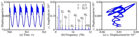
Figure 19.
Periodic-n motion of RBRS at ω = 19.2 rad/s: (a) Waveform, (b) Frequency, and (c) Axis orbit and Poincaré map.
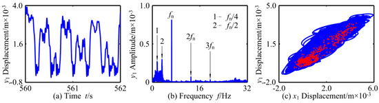
Figure 20.
Chaotic motion of RBRS at ω = 40.8 rad/s: (a) Waveform, (b) Frequency, and (c) Axis orbit and Poincaré map.
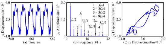
Figure 21.
Periodic-4 motion of RBRS at ω = 69.8 rad/s: (a) Waveform, (b) Frequency, and (c) Axis orbit and Poincaré map.
3.4. Influence of Friction Coefficient on Dynamic Characteristics of RBRS under Variable Speed
Friction coefficient μ has an important influence on the dynamic behavior of RBRS, and its size directly affects the dynamic characteristics of the coupling system. Figure 22, Figure 23, Figure 24, Figure 25, Figure 26 and Figure 27 show the dynamic response (bifurcation diagram and three-dimensional spectrum diagram) of the system under different working conditions when the rotational speed is in the range of ω ∈ [7.0,71.0] rad/s and the friction coefficient is μ = 0.05, μ = 0.3, and μ = 0.78, respectively. By comparison it can be seen that when the friction coefficient is small, that is, μ = 0.05, the RBRS in the interval of ω ∈ [7.0,60.2] rad/s mainly exhibits the period-1 motion, and the response amplitude is relatively stable (when ω = 51.2 rad/s, the coupling system behaves as chaotic motion; when ω = 52.6 rad/s, the coupling system behaves as a period-3 motion), and there are many obvious discontinuous amplitude jumps. With the increase of the rotational speed, the system transits from periodic motion to chaotic motion through saddle-node bifurcation at ω = 60.4 rad/s, and exhibits multiple motion states including periodic-1, periodic-2, periodic-n, Quasi-periodic, and chaotic motion. The coupling system appears as intermittent chaos, with the saddle-node bifurcation, the period-doubling bifurcation, and the inverse period-doubling bifurcation appearing alternately. In addition to the frequency multiplication component in the three-dimensional spectrum, there are also frequency demultiplication components (fn/2, 3 fn/25, fn/7,...) and continuous spectrum components; when μ = 0.3, the dynamic characteristics of the coupling system become more complex and the chaotic movement is strengthened. At lower rotational speeds, the jump of the coupling system is weakened, and the motion state returns to the stable periodic motion at 21.0 < ω < 27.8 rad/s again from the periodic motion in the range of ω ∈ [7.0,20.0] rad/s through the chaotic motion in the narrow interval ω ∈ [20.2,21.0] rad/s. When ω > 27.8 rad/s, the system enters the chaotic region through the saddle-node bifurcation, and the periodic motion, the quasi-periodic motion, and the chaotic motion appear alternately until ω = 61.4 rad/s. When 61.4 rad/s <ω < 63.2 rad/s, RBRS is in stable period-4 motion and period-8 motion and is accompanied by the occurrence of inverse period-doubling bifurcation; the three-dimensional spectrum shows distinct frequency demultiplication components of fn/4 and fn/8, and RBRS re-enters into the chaotic region at ω = 63.2 rad/s through the saddle-node bifurcation; when the friction coefficient is increased to μ = 0.78, while ω < 28.0 rad/s, the vibration system performs chaotic motion and periodic multiple motion alternatively only in the narrow interval ω ∈ [21.8,24.8] rad/s, and in other cases perform stable periodic motion. With the increase of the rotational speed, the system enters the unsteady region through the saddle-node bifurcation at ω = 28.2 rad/s. The system alternates frequently between the period-doubling motion, the counter-periodic motion, and the chaotic motion, and the jumping discontinuity of the response amplitude is intensified. Table 5 shows the intervals in which the frequency components change (where fn is the frequency conversion).
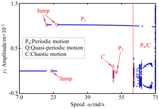
Figure 22.
The bifurcation diagram of RBRS at μ = 0.05.
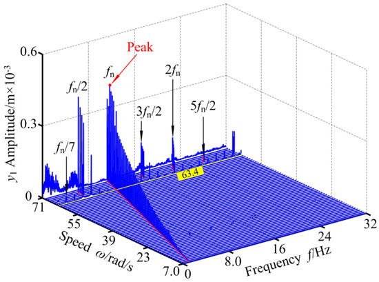
Figure 23.
3-D frequency spectrum of RBRS at μ = 0.05.
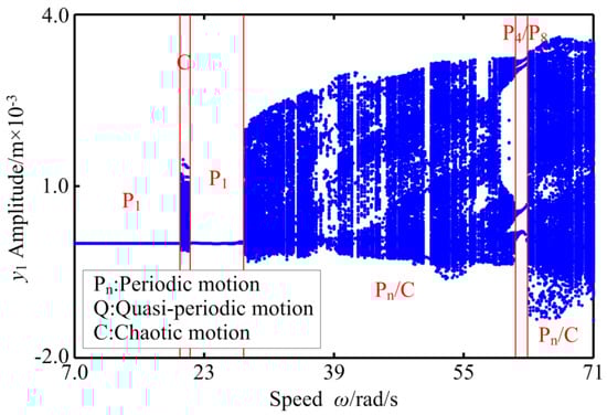
Figure 24.
The bifurcation diagram of RBRS at μ = 0.3.
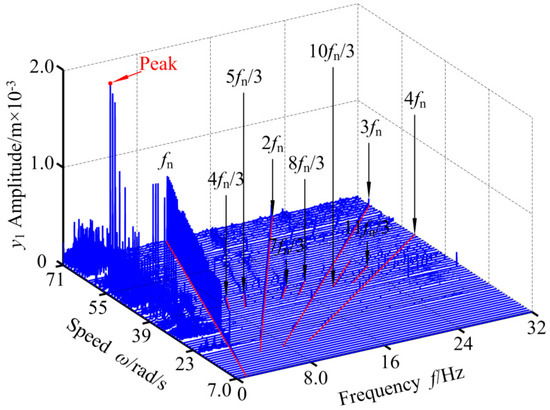
Figure 25.
3-D frequency spectrum of RBRS at μ = 0.3.
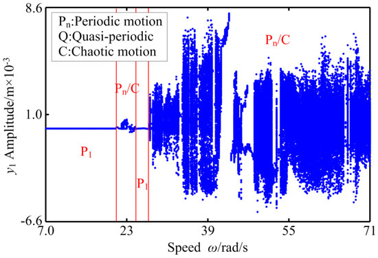
Figure 26.
The bifurcation diagram of RBRS at μ = 0.78.
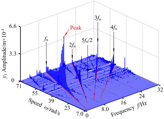
Figure 27.
3-D frequency spectrum of RBRS at μ = 0.78.
Table 5.
Frequency feature of RBRS under different friction coefficient.
In order to better display the influence of friction coefficient μ on the dynamic characteristics of the system, Figure 28, Figure 29 and Figure 30 show that the time domain map, frequency domain map, axis orbit map, and Poincaré map of the coupling system with μ = 0.78, when ω = 29.8 rad/s, ω = 43.2 rad/s and ω = 52.2 rad/s, respectively. It can be seen from the Figure 28, Figure 29 and Figure 30 that the vibration response of the three cases are nonlinear; in the frequency domain, fn, 2fn, and 3fn are the main frequency components, and there are frequency multiplication and frequency demultiplication components whose amplitude is not obvious. In addition, the axis orbit map changes from chaotic closed curves to multiple non-coincident closed curves, and then to five closed ones; and the attractors on the corresponding Poincaré map show irregular scatters, isolated multiple points, and isolated five points, respectively. Then the system completes the alternative evolution of chaotic motion, periodic-n motion, and period-5 motion.
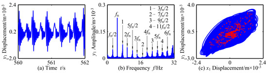
Figure 28.
Chaotic motion of RBRS at ω = 29.8 rad/s: (a) Waveform, (b) Frequency, and (c) Axis orbit and Poincaré map.
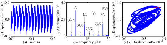
Figure 29.
Periodic-n motion of RBRS at ω = 43.2 rad/s: (a) Waveform, (b) Frequency, and (c) Axis orbit and Poincaré map.
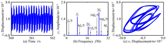
Figure 30.
Periodic-5 motion of RBRS at ω = 52.2 rad/s: (a) Waveform, (b) Frequency, and (c) Axis orbit and Poincaré map.
Based on the above numerical simulation, it can be seen that the friction coefficient μ is an important parameter affecting the dynamic characteristics of the coupling system (RBRS). With the increase of the friction coefficient, the motion state of the system becomes more complex, the chaotic region increases first and then decreases, the complex motion and periodic motion alternate frequently, and the response amplitude increases gradually.
4. Conclusions
In this paper, a model considering multiple nonlinear factors is proposed. The complex nonlinear dynamic behavior of the coupling system is studied. The influence of the excitation current, radial stiffness, and friction coefficient on the dynamic characteristics of RBRS is analyzed. The following conclusions can be drawn from the study.
- (1)
- For the RBRS coupling system, with the change of parameters, there are many kinds of motion states, including periodic-n, quasi-periodic, and chaotic motion. At the same time, the coupling system has intermittent chaos many times, and Hopf, saddle-node, period-doubling, and inverse period-doubling bifurcation appear alternately. The dynamic properties of the coupling system caused by different nonlinear factors are interactional.
- (2)
- When the excitation current of the generator Ij is small, the dynamic behavior of the system is relatively simple. As the rotational speed increases, the system transits from short-term periodic motion, chaotic motion, and quasi-periodic motion to periodic motion, successively undergoing saddle-node bifurcation, period-doubling bifurcation, inverse period-doubling bifurcation, and Hopf bifurcation. The increase of the excitation current Ij can inhibit the response amplitude of the system to some extent, but it cannot inhibit the motion state of the system, which makes the motion state of the system more complex, the chaotic motion wider, and the jump discontinuity enhanced. At higher speeds, the number of high-order bifurcation increases as the excitation current Ij increases.
- (3)
- Due to the influence of the radial stiffness kr and the friction coefficient, the coupled system shows more complex nonlinear behavior. With the increase of radial stiffness kr, the motion complexity of the coupling system increases, the chaotic region increases, the response amplitude increases, and the vibration intensity increases. At the same time, in the high-speed region, the periodic motion region becomes narrow and tends to disappear. With the increase of the friction coefficient, the chaotic region increases first and then decreases, the complex motion and periodic motion alternate frequently, and the response amplitude increases gradually.
Author Contributions
The topic of this research is designed by Y.L.; Formal analysis is completed by Y.L.; The first version manuscript is prepared by Y.L.; and this version of the manuscript is read, approved and substantially contributed by Y.L., Z.H., H.L., G.S.
Funding
This research was funded by Fundamental Research Funds for the Central Universities (Grant number N170303008).
Conflicts of Interest
The authors declare no conflict of interest.
References
- Ma, Z.Y.; Dong, Y.X. Dynamics of Water Turbine Generator Set; University of Technology: Dalian, China, 2003. [Google Scholar]
- Wen, B.C. Nonlinear Vibration of Engineering; Science: Beijing, China, 2007. [Google Scholar]
- Chu, F.; Lu, W. Experimental observation of nonlinear vibrations in a rub-impact rotor system. J. Sound Vib. 2005, 283, 621–643. [Google Scholar] [CrossRef]
- Patel, T.H.; Darpe, A.K. Coupled bending-torsional vibration analysis of rotor with rub and crack. J. Sound Vib. 2009, 326, 740–752. [Google Scholar] [CrossRef]
- Cao, J.; Ma, C.; Jiang, Z.; Liu, S. Nonlinear dynamic analysis of fractional order rub-impact rotor system. Commun. Nonlinear Sci. Numer. Simul. 2011, 16, 1443–1463. [Google Scholar] [CrossRef]
- Huang, Z.; Zhou, J.; Yang, M.; Zhang, Y. Vibration characteristics of a hydraulic generator unit rotor system with parallel misalignment and rub-impact. Arch. Appl. Mech. 2011, 81, 829–838. [Google Scholar] [CrossRef]
- Ma, H.; Shi, C.; Han, Q.K.; Wen, B.C. Fixed-point rubbing fault characteristic analysis of a rotor system based on contact theory. Mech. Syst. Signal Process. 2013, 38, 137–153. [Google Scholar] [CrossRef]
- Khanlo, H.M.; Ghayour, M.; Ziaei-Rad, S. The effects of lateral-torsional coupling on the nonlinear dynamic behavior of a rotating continuous flexible shaft-disk system with rub-impact. Commun. Nonlinear Sci. Numer. Simul. 2013, 18, 1524–1538. [Google Scholar] [CrossRef]
- Jacquet-Richardet, G.; Torkhani, M.; Cartraud, P.; Thouverez, F.; Nouri Baranger, T.; Herran, M.; Gibert, C.; Baguet, S.; Almeida, P.; Peletan, L. Rotor to stator contacts in turbomachines. Review and application. Mech. Syst. Signal Process. 2013, 40, 401–420. [Google Scholar] [CrossRef]
- Lu, W.; Chu, F. Radial and torsional vibration characteristics of a rub rotor. Nonlinear Dyn. 2014, 76, 529–549. [Google Scholar] [CrossRef]
- Ma, H.; Zhao, Q.; Zhao, X.; Han, Q.K.; Wen, B.C. Dynamic characteristics analysis of a rotor-stator system under different rubbing forms. Appl. Math. Modell. 2015, 39, 2392–2408. [Google Scholar] [CrossRef]
- Xiang, L.; Gao, X.; Hu, A. Nonlinear dynamics of an asymmetric rotor-bearing system with coupling faults of crack and rub-impact under oil-film forces. Nonlinear Dyn. 2016, 86, 1057–1067. [Google Scholar] [CrossRef]
- Ma, H.; Lu, Y.; Wu, Z.; Tai, X.; Wen, B.C. Vibration response analysis of a rotational shaft-disk-blade system with blade-tip rubbing. Int. J. Mech. Sci. 2016, 107, 110–125. [Google Scholar] [CrossRef]
- Ma, H.; Yin, F.; Tai, X.; Wang, D.; Wen, B.C. Vibration response analysis caused by rubbing between rotating blade and casing. J. Mech. Sci. Technol. 2016, 30, 1983–1995. [Google Scholar] [CrossRef]
- Mokhtar, M.A.; Kamalakar Darpe, A.; Gupta, K. Investigations on bending-torsional vibrations of rotor during rotor-stator rub using Lagrange multiplier method. J. Sound Vib. 2017, 401, 94–113. [Google Scholar] [CrossRef]
- Yang, Y.; Cao, D.; Wang, D.; Jiang, G. Response analysis of a dual-disc rotor system with multi-unbalances-multi-fixed-point rubbing faults. Nonlinear Dyn. 2017, 87, 109–125. [Google Scholar] [CrossRef]
- Yang, Y.; Cao, D.; Wang, D. Investigation of dynamic characteristics of a rotor system with surface coatings. Mech. Syst. Signal Process. 2017, 84, 469–484. [Google Scholar] [CrossRef]
- Yang, B.S.; Kim, Y.H.; Son, B.G. Instability and Imbalance Response of Large Induction Motor Rotor by Unbalanced Magnetic Pull. J. Vib. Control 2004, 10, 447–460. [Google Scholar] [CrossRef]
- Gustavsson, R.K.; Aidanpää, J.O. The influence of nonlinear magnetic pull on hydropower generator rotors. J. Sound Vib. 2006, 297, 551–562. [Google Scholar] [CrossRef]
- Perers, R.; Lundin, U.; Leijon, M. Saturation Effects on Unbalanced Magnetic Pull in a Hydroelectric Generator with an Eccentric Rotor. IEEE Trans. Magn. 2007, 43, 3884–3890. [Google Scholar] [CrossRef]
- Lundström, N.L.P.; Aidanpää, J.O. Dynamic consequences of electromagnetic pull due to deviations in generator shape. J. Sound Vib. 2007, 301, 207–225. [Google Scholar] [CrossRef]
- Calleecharan, Y.; Aidanpää, J.O. Dynamics of a hydropower generator subjected to unbalanced magnetic pull. Proc. Inst. Mech. Eng. Part C J. Mech. Eng. Sci. 2011, 225, 2076–2088. [Google Scholar] [CrossRef]
- Xu, Y.; Li, Z. Computational Model for Investigating the Influence of Unbalanced Magnetic Pull on the Radial Vibration of Large Hydro-Turbine Generators. J. Vib. Acoust. 2012, 134, 051013. [Google Scholar] [CrossRef]
- Zeng, Y.; Zhang, L.; Guo, Y.; Qian, J.; Zhang, C. The generalized Hamiltonian model for the shafting transient analysis of the hydro turbine generating sets. Nonlinear Dyn. 2014, 76, 1921–1933. [Google Scholar] [CrossRef]
- Xu, B.; Chen, D.; Zhang, H.; Zhou, R. Dynamic analysis and modeling of a novel fractional-order hydro-turbine-generator unit. Nonlinear Dyn. 2015, 81, 1263–1274. [Google Scholar] [CrossRef]
- Xu, X.; Han, Q.; Chu, F. Nonlinear vibration of a generator rotor with unbalanced magnetic pull considering both dynamic and static eccentricities. Arch. Appl. Mech. 2016, 86, 1521–1536. [Google Scholar] [CrossRef]
- Xiang, C.; Liu, F.; Liu, H.; Han, L.; Zhang, X. Nonlinear dynamic behaviors of permanent magnet synchronous motors in electric vehicles caused by unbalanced magnetic pull. J. Sound Vib. 2016, 371, 277–294. [Google Scholar] [CrossRef]
- Li, R.; Li, C.; Peng, X.; Wei, W.; Sciubba, E. Electromagnetic Vibration Simulation of a 250-MW Large Hydropower Generator with Rotor Eccentricity and Rotor Deformation. Energies 2017, 10, 2155. [Google Scholar] [CrossRef]
- Yan, D.; Zhuang, K.; Xu, B.; Chen, D.; Mei, R.; Wu, C.; Wang, X. Excitation Current Analysis of a Hydropower Station Model Considering Complex Water Diversion Pipes. J. Energy Eng. 2017, 143, 04017012. [Google Scholar] [CrossRef]
- Bathe, K.J.; Wilson, E.L. Numericalmethodsin Finite Elementanalysis; Prentice-Hall Inc.: Upper Saddle River, NJ, USA, 1976. [Google Scholar]
- Zhou, J.Z.; Zhang, Y.C.; Li, C.S. Dynamic Problems and Fault Diagnosis Principles Methods of Hydroelectric Generating Set; Huazhong University of Science and Technology: Wuhan, China, 2013. [Google Scholar]
© 2019 by the authors. Licensee MDPI, Basel, Switzerland. This article is an open access article distributed under the terms and conditions of the Creative Commons Attribution (CC BY) license (http://creativecommons.org/licenses/by/4.0/).