Augmenting GPS with Geolocated Fiducials to Improve Accuracy for Mobile Robot Applications

Abstract

In recent decades Global Positioning Systems (GPS) have become a ubiquitous tool to support navigation. Traditional GPS has an error in the order of 10–15 m, which is adequate for many applications (e.g., vehicle navigation) but for many robotics applications lacks required accuracy. In this paper we describe a technique, FAGPS (Fiducial Augmented Global Positioning System) to periodically use fiducial markers to lower the GPS drift, and hence for a small time-period have a more accurate GPS determination. We describe results from simulations and from field testing in open-sky environments where horizontal GPS accuracy was improved from a twice the distance root mean square (2DRMS) error of 5.5 m to 2.99 m for a period of up-to 30 min.

1. Introduction

GPS (Global Positioning System) is a global absolute navigation system which uses one-way time of arrival (TOA) ranging from a constellation of satellites to compute a reasonably accurate three-dimensional position [1]. Since the removal of selective availability in 2000 (which significantly improved accuracy) and the inclusion of GPS receivers in most smartphones, GPS has become a near ubiquitous system, particularly when paired with GIS (Global Information Systems) for navigation and mapping services. GPS is also used as a precision timing reference across a variety of industries including synchronization of cell towers, timestamping financial transactions and synchronising scientific instruments [2].

GPS (originally known as NAVSTAR GPS) is the oldest Global Navigation Satellite System (GNSS) with planning and development starting in the early 1960’s leading to full operational capacity, with a constellation of 24 satellites, being reached in 1995. A number of alternate systems exist or are being developed including the Russian Global Navigation Satellite System (GLONASS), the European GALILEO system and the Chinese BeiDou Navigation Test System (BNTS). Although the majority of low cost receivers currently only support traditional GPS, the proliferation of these additional constellations and the prospect of improved positional accuracy has lead to the development of GNSS receivers which can provide positional estimates by augmenting data across a range of different satellite constellations [3].

GPS has several sources of error which effect accuracy including changing atmospheric conditions, multipath, clock discrepancies and receiver noise [4,5,6,7,8]. These error sources each contribute with different time horizons. For example multipath effects (where the receiver receives both direct and reflected signals) may be relatively static in nature but then may change rapidly in the case of moving receivers and significant changes in the environment (e.g., the closing of a stadium roof) [7].

In contrast, atmospheric errors (ionospheric and tropospheric) tend to change more slowly. Atmospheric errors are caused by changes in atmospheric conditions (e.g., temperature, humidity, pressure) which contribute to varying degrees based on satellite elevation [8]. Likewise orbital errors and satellite clock errors also have relatively slow changes over time [6,8].

Besides using other constellations there are a number of technologies used in the augmentation of traditional GPS to improve performance. These technologies include Assisted GPS (AGPS) to improve cold start performance, Differential GPS (DGPS) to reduce error and Inertial Navigation Systems (INS) to provide navigation in GPS denied areas [9,10].

An alternate scheme to DGPS (but not as accurate), WAAS (Wide Area Augmentation Schemes) involves geostationary satellites broadcasting correction data based on a network of widely dispersed ground based stations [1]. Another correction approach is to use Real Time Kinematic GPS (RTK-GPS) which produces highly accurate navigation with a close (within 10 km) base station transmitting correction data over a radio link [11].

DGPS systems have seen widespread use where greater precision is required than traditional GPS. This includes applications such as precision farming (with GPS guided machinery) and marine navigation [12].

Fiducial markers are artificial landmarks which are added to a scene to facilitate registration of points in images or between images and a known model [13]. Fiducial markers are commonly used with pose estimation for robot navigation, biomedical image registration, augmented reality applications and industrial applications (e.g., PCB fabrication) [14,15,16].

Fiducials have previously been used in GPS-denied environments to augment odometry and inertial navigation systems (INS) to facilitate more accurate navigation through association with a ground-truth [17,18,19]. In contrast, we propose to use fiducials regions in non-GPS denied environments to improve GPS accuracy by reducing errors associated with time-variant variables for a short period of time. Our technique, FAGPS (Fiducial Augmented GPS), which augments traditional GPS data with position data acquired from a stationary geo-referenced fiducial marker. Hence, for a time interval in the order of 20–30 min a more accurate position determination is achieved. We validate FAGPS through empirical studies and simulation based on corrections of GPS data for stationary and moving GPS receivers.

This paper is structured as follows: Section 2 covers some of the related research in the fields of GPS augmentation using DGPS techniques and an overview of fiducial markers. Following this Section 3 describes the proposed FAGPS scheme. Section 4 describes the experiments used to validate FAGPS followed by the experimental results and a discussion in Section 5. Finally, Section 6 provides some concluding remarks.

2. Related Research

This section provides background to existing technologies used to improve GPS performance and fiducial techniques.

Assisted-GPS (AGPS) is a technique which uses a non-GPS radio signals (e.g., WIFI locations, cell tower beacons) to significantly improve GPS cold start time as these radio signals help coarsely localise the GPS receiver. Once the navigation unit knows its approximate location (within a few kilometres) the GPS receiver can more rapidly determine the precise position [20]. An additional advantage of AGPS is that it helps guard against GPS spoofing (when a GPS signals are maliciously spoofed) as all of the relevant cell tower beacons or WIFI locations would also have to be spoofed.

Differential-GPS (DGPS) uses a fixed ground based GPS beacon as a reference point [21]. The beacon computes the error measurement between the measured GPS point and the known beacon position. This error is predominately due to atmospheric conditions and hence can be used by local DGPS receivers to correct for errors. The distance to the beacon is an important factor with each increase of 100 km resulting in an error of 0.2 m [10] and so for best performance the DGPS receiver should be relatively close to the beacon. DGPS receives regular beacon updates (typically in the order of 5 min) to ensure that recent data is being used to correct GPS signals.

Like traditional GPS, DGPS is susceptible to spoofing and jamming. For applications which require the precision of DGPS (e.g., autonomous farming, marine navigation) this reduction in accuracy may have catastrophic consequences [22].

One more recent development is internet based DGPS, which is targeted to applications where a GPS receiver is connected to the internet and can receive differential update information online. Such systems are well suited to mobile phone applications where GPS and 4G are tightly coupled together [23,24].

Table 1. Summary of horizontal error for different augmentation techniques.

Data Point	Horizontal Error	Notes
Global Positioning System (GPS)	10–15 m [25]	No augmentation
Wide Area Augmentation System (WAAS)	2–5 m [25]	Availability subject to location
Differential Global Positioning System (DGPS)	<1 m [10]	Accuracy depends on distance to beacon

summarises positional error for different GPS augmentation schemes. Although the DGPS scheme provides the most accuracy it is also the highest cost (receivers are several orders of magnitude more expensive than traditional GPS receivers).

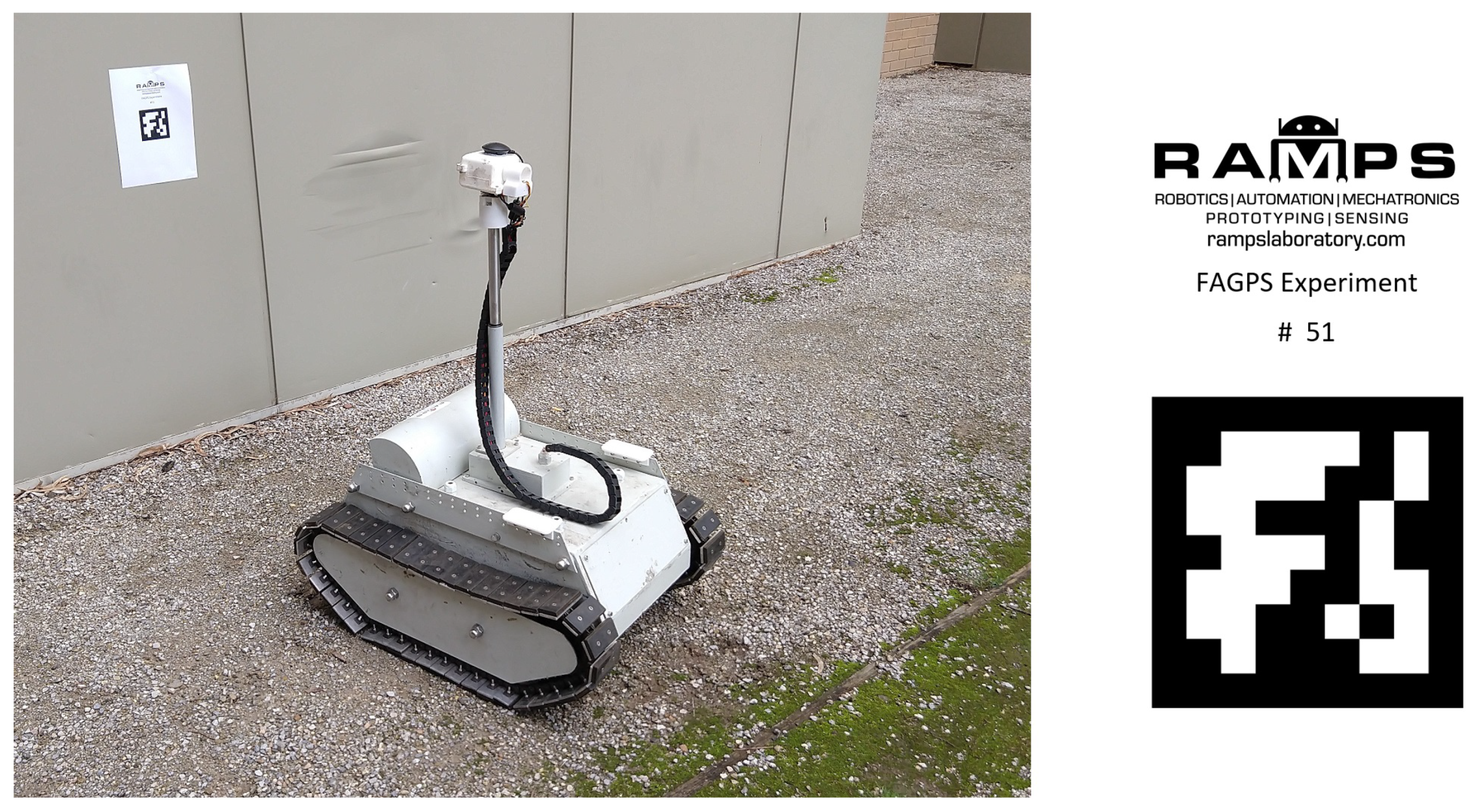
Central to the concept of FAGPS is the pose estimation based on georeferenced landmarks or fiducial points. In terms of fiducial points, the proposed FAGPS system could conceivably operate both with traditional 2D fiducial images and with so-called real-world fiducials. 2D Fiducial images are high contrast, black and white images of known size and content which are placed in an environment to facilitate pose estimation (as shown in Figure 1) [26].

Real-world fiducials are natural or man-made structures not designed for the purpose of machine vision waypoints, but can be used for this task [27]. Some examples of real-world fiducials include: a corner in a fence or building and key features in a path or structure which have been accurately georeferenced to a map. These real-world fiducials are generally difficult to automatically detect reliably (even artificial fiducials can be difficult to detect in real-world environments) [28]. The constrained search size (expectation that a fiducial is within a certain area given the non-compensated GPS margin of error) should help improve detection and reduce false positives. The other issue with many of these real-world fiducials is the quality of pose-estimation, which can be very accurate given a completely flat, high contrast 2D artificial fiducial (Figure 1), but less so for a real-world fiducial not optimised for post-estimation.

The technique proposed in this paper, FAGPS, performs a similar role to DGPS and RTK-GPS in using a ground based georeferenced landmark to compensate for common mode errors. FAGPS uses close-by fiducials (similar to RTK-GPS) but in contrast to DGPS and RTK-GPS doesn’t require any transmitter hardware at the beacon points (only a georeferenced fiducial marker), which means many beacons can be quickly created at very low cost and require no power. Receivers using the FAGPS scheme will need to be coupled with a machine vision platform to allow them to recognise and perform pose estimation on the landmarks. Some operational downtime is experienced as FAGPS receivers will need to physically go to a beacon to receive calibration coordinates at regular intervals.

3. Proposed Technique

The FAGPS technique proposed in this paper is to augment the GPS measurement with a georeferenced fiducial marker which a robot may observe within the environment and perform pose-estimation on. Hence, once calibrated, for a short time interval, the robot can use this augmentation to reduce positional error. Unlike DGPS which requires a costly DGPS receiver along with a differential beacon the proposed FAGPS scheme requires no hardware on the ground, doesn’t require access to power and uses the same low cost commercial receiver used by the robot itself.

As the robot needs to directly observe (and perform pose estimation on) the geolocated fiducial, this limits the effective range the robot can be away from the reference point based on how quickly the robot can travel within the increased accuracy timeframe. To expand the area of operation a series of geolocated fiducials could be deployed—when the robot needs to re-acquire a fiducial it can go to the closest one.

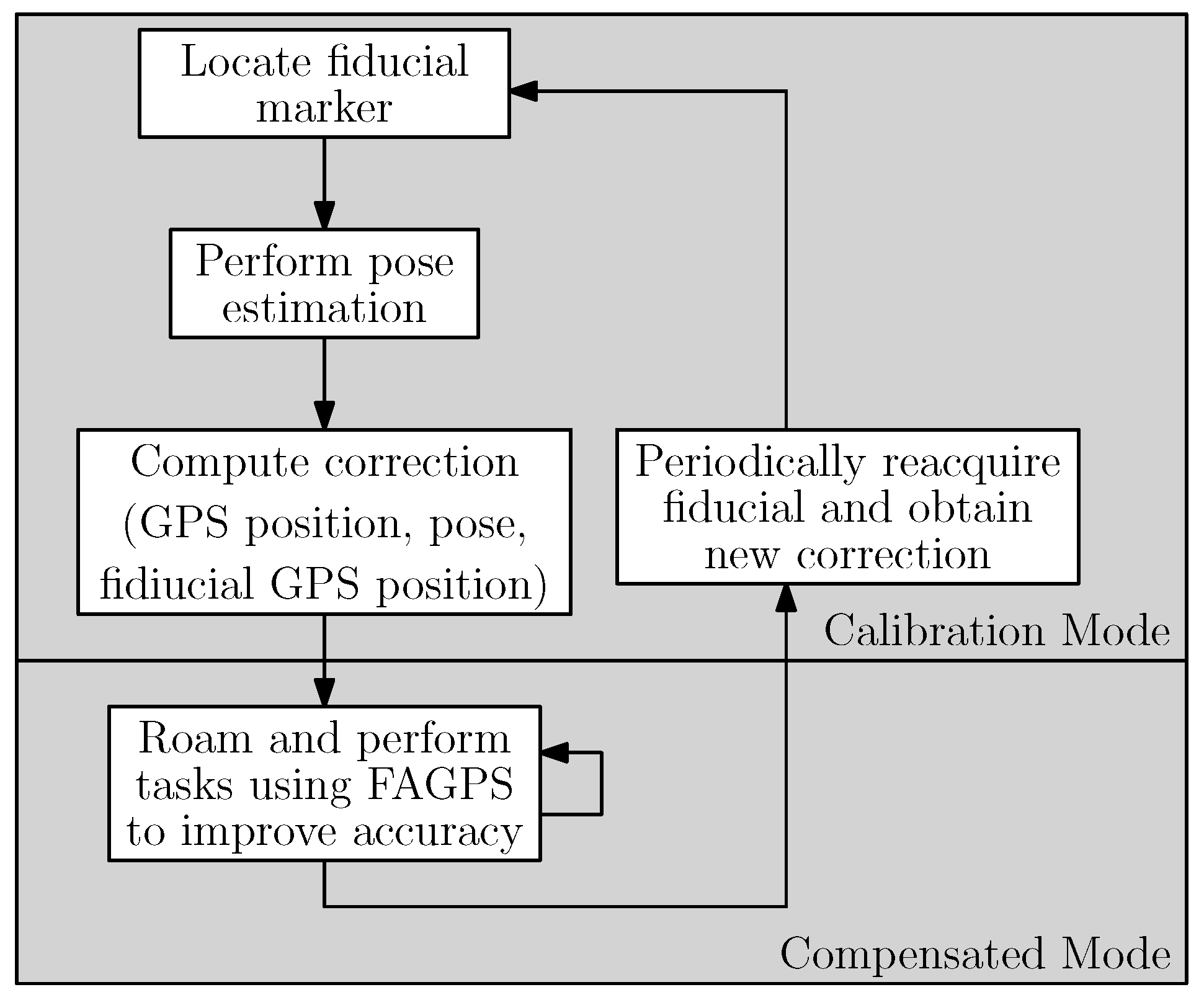
The FAGPS approach we have proposed operates in two modes: a calibration mode and a compensated mode as shown in Figure 2. The calibration mode is where the FAGPS approach captures and aligns a GPS position (Latitude, Longitude, Altitude) with a visual reference point. In a practical robot system this could involve a ground robot driving up to a fiducial marker or a helicopter robot hovering and performing pose estimation above a fiducial marker (or a natural visual feature like the corner of a fence) and capturing the GPS coordinates at this point.

The calibration mode first involves locating the fiducial marker. As the uncompensated GPS measurement will suffer from significant inaccuracies, the robot (or measurement platform) should approach the approximate location at a distance of 10’s of meters and use machine vision try to locate the position of the fiducial. Once this operation has been performed the robot can approach the fiducial more closely (Euclidean distance less than 5 m) to facilitate a more accurate pose estimation measurement. Once this pose estimation has been performed, GPS calibration coordinates can be captured and calibration offsets will be calculated as specified in Equations (1) and (2).

$$x_{tc}=x_t-(x-x_0)$$

(1)

$$y_{tc}=y_t-(y-y_0)$$

(2)

where x and y refer to the respective latitude and longitude of the robot computed with pose estimation from the geolocated reference point. $x_0$ and $y_0$ refer to the GPS position received when pose estimation occurred. $x_t$ and $y_t$ refers to the current received GPS position at time t. $x_{tc}$ and $y_{tc}$ refers to the FAGPS corrected coordinates at time t.

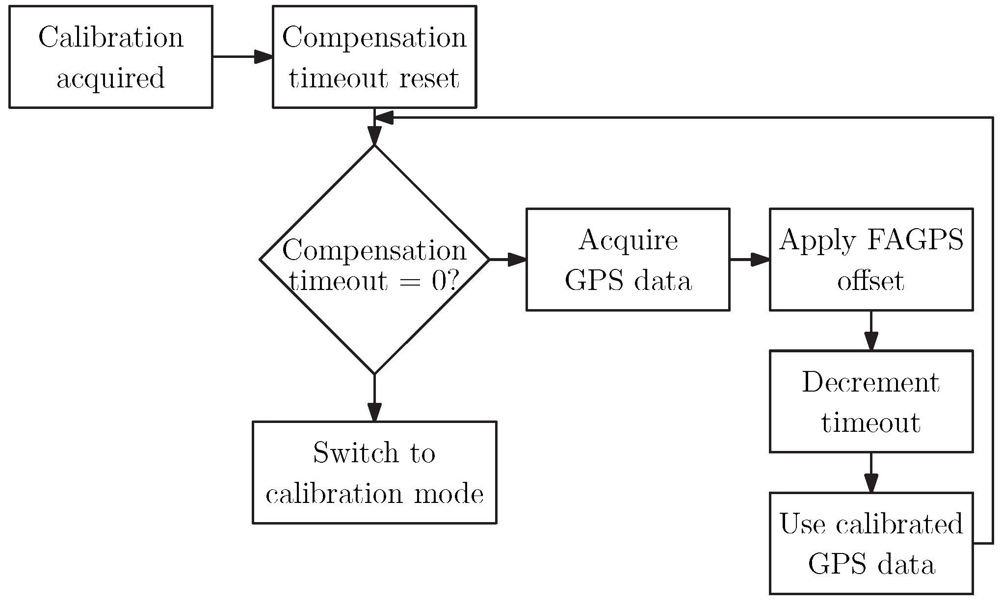
Once these calibration coordinates have been captured the robot will operate in the compensated mode as outlined in Figure 3. In the compensated mode the FAGPS acquired calibration offsets are applied to all new GPS data to improve accuracy. It is expected that the area of operation will be relatively small (as this is primarily designed to improve the navigation performance for small unmanned robots), so an area of operation within 10 km should be reasonable.

The other problem relates to the time interval before reacquiring a FAGPS compensated point as changing atmospheric conditions will increase uncertainty over time. The process of reacquisition is easy and efficient to do in a This has been improved in the introduction with references and descriptions of the sources of error over time relating to drift over time and why this causes the aging of the correction values. DGPS scheme (typically performed at most every few minutes) but for the proposed FAGPS technique it requires going back to and reacquiring calibration data from a fiducial point. One way to improve efficiency of calibration reacquisition would be to have a series of fiducial points and the robot can each time go to the closest point to reacquire data. Alternately this system could work effectively for a swarm of robots where periodically the robot closest to (or most underutilized) could reacquire calibration coordinates and share them with the rest of the swarm.

The proposed technique shares some attributes with traditional DGPS, most notably that although there is accuracy improvement through improving common mode noise (e.g., introduced by satellites and stratosphere), non common mode noise like multipath interference around buildings will not be improved. One advantage the proposed FAGPS technique has over DGPS is that the same receiver is used for computing the calibration coordinates as what is used for navigation—so any difference in the receiver performance between a DGPS beacon and the mobile receiver is negated.

4. Test Procedure

This section describes a simulation and three experiments which are designed to model time-dependent varying errors, determine the baseline accuracy from a low-cost commercial GPS receiver, to assess the improvement in accuracy using the proposed FAGPS system using both a static system and a mobile robot platform.

4.1. Simulation

As the corrections in the scheme have a time dependency associated with them (the correction values age based on changes in common mode noise like changes in atmospheric conditions). We performed simulations to evaluate this growing uncertainty of the corrections over time. The simulation involves 2000 data points for each of the FAGPS and non-FAGPS schemes. These data points were simulated to contain both elements of Gaussian noise ($Z_{ix}$ and $Z_{iy}$ simulating the general noise in GPS signals) and Gaussian noise with a time dependency ($Z_{itx}$ and $Z_{ity}$ simulating the aging of correction data).

Hence, the FAGPS (3) and non-FAGPS (4) data sets are computed as follows:

$$\begin{array}{cc}\hfill & FAGPS{x}_i=Z_{ix}+Z_{itx}\hfill \\ \hfill & FAGPS{y}_i=Z_{iy}+Z_{ity}\hfill \end{array}$$

(3)

$$\begin{array}{cc}\hfill & GPS{x}_i=Z_{ix}+Z_{itx}+x_0\hfill \\ \hfill & GPS{y}_i=Z_{iy}+Z_{ity}+y_0\hfill \end{array}$$

(4)

where $Z_{ix}$ and $Z_{iy}$ are Gaussian noise with $\mu =0$ and ${\sigma }^2=0.5$. $Z_{igx}$ and $Z_{igy}$ are time increasing Gaussian noise variables with $\mu =0$ and ${\sigma }^2=i/1000$. Finally $x_0$ = 0.75 m and $y_0$ = 0.5 m and are added onto the non-FAGPS data set to show an initial error offset corrected by the FAGPS scheme.

4.2. Experiment 1—Static Repeatability

The first experiment was designed to provide a measure of the accuracy performance of a static commercial GPS receiver. This accuracy will be used as a baseline for the other experiments to determine the drift associated with GPS measurement in different conditions.

A EM-406A SiRF III GPS receiver was interfaced with a microcontroller which was programmed to periodically log the GPS data to flash memory. The receiver was placed outside in a static position with clear line of sight of the sky for a period of approximately 44 h, logging a total of 162,676 measurements through different weather and atmospheric conditions. The sampled results for Latitude and Longitude are presented in Section 5.2.

4.3. Experiment 2—Spatial Displacement Repeatability

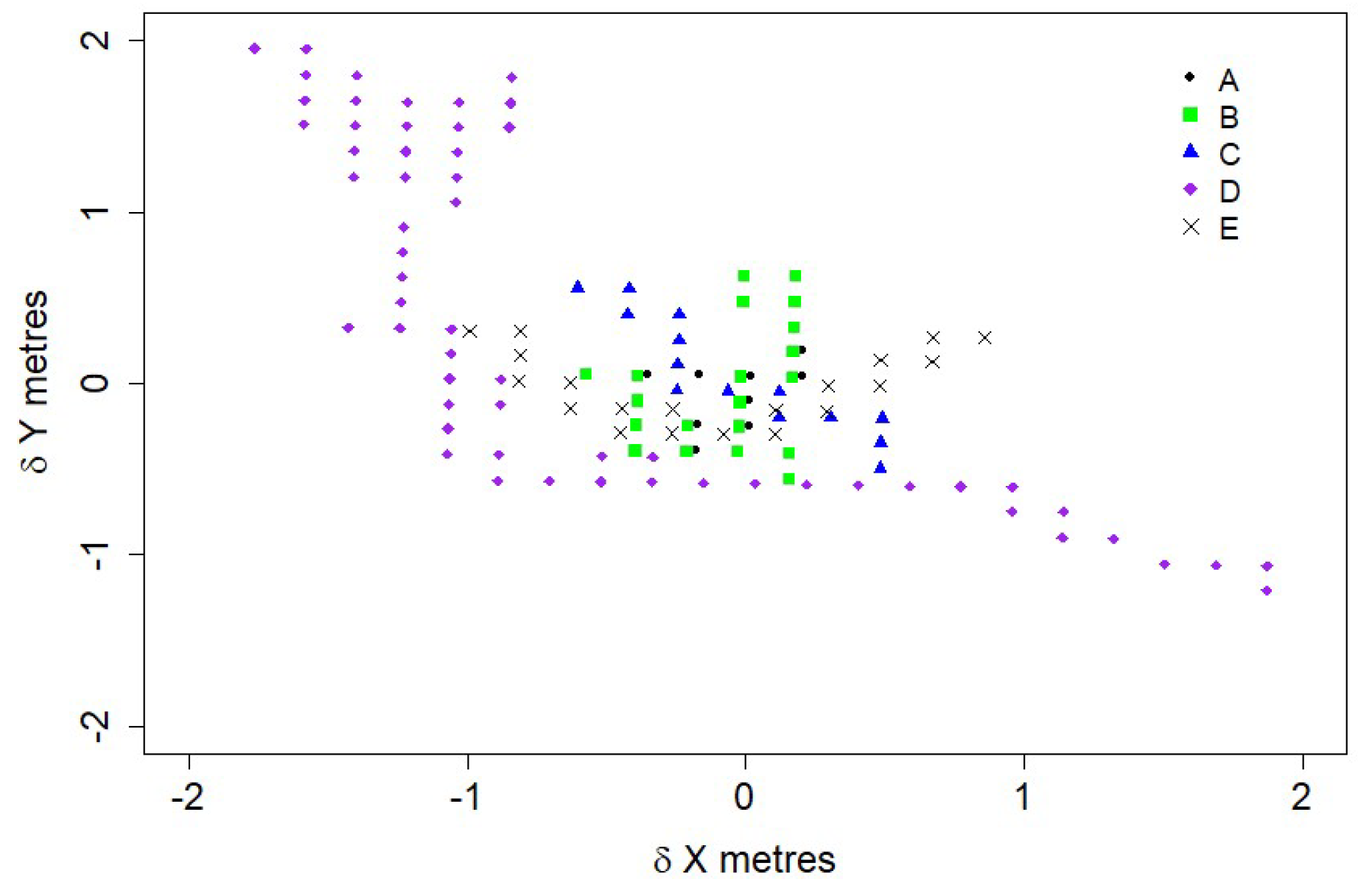
The purpose of the second experiment was to validate the efficacy of the FAGPS technique over a short range real-world environment with both multipath and non-multipath errors present. Hence, the aim of this experiment is to verify that performing a calibration at one geolocated landmark should improve GPS performance when the receiver is moved and tested at another point (for a limited period of time).

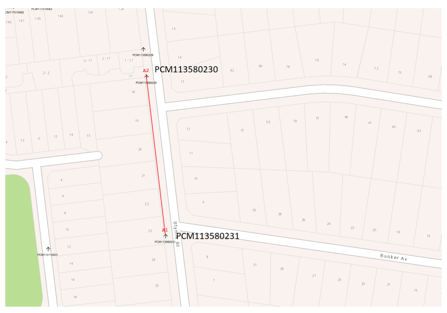
Two survey points were identified (

Table 2. Locations of survey points.

Survey Point Name	Latitude	Longitude
PCM113580231	−37.71373333	145.02958889
PCM113580230	−37.71371667	145.02958333

and Figure 4) and located. These survey points were approximately 95 m apart and are located in a residential area.

The first survey point (PCM113580231) was selected as the geolocated reference point. The GPS was turned on at survey point PCM113580231 and was left static for 5 min to ensure that it had a reliable fix. Based on the known position of PCM113580231 the measured position offsets in X and Y were computed to correct the data (latitude offset = 0.0000546667, longitude offset = 0.0000326667).

The GPS receiver was then repositioned at PCM113580230 for an hour in order to assess the performance of the correction over time at a different survey point.

4.4. Experiment 3—Mobile Repeatability for Robot Applications

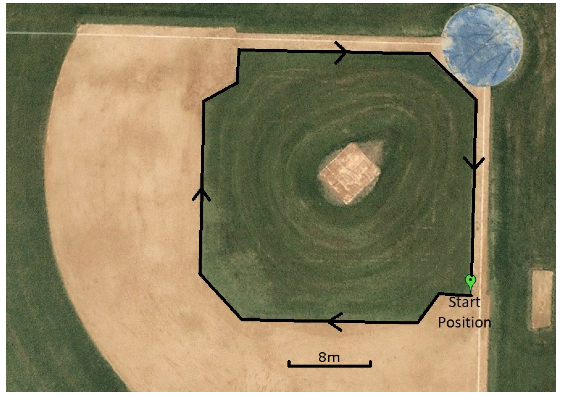
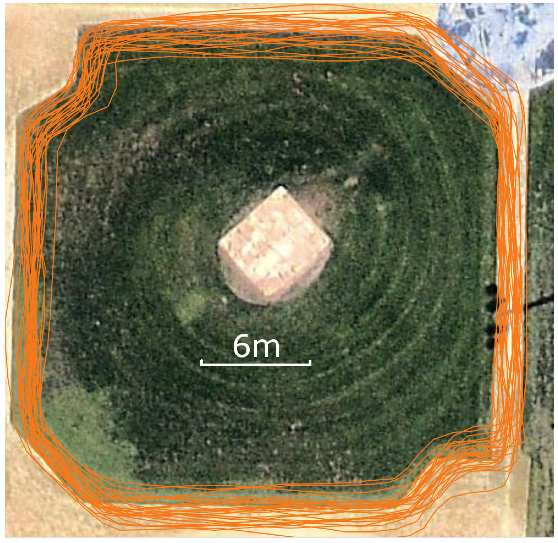
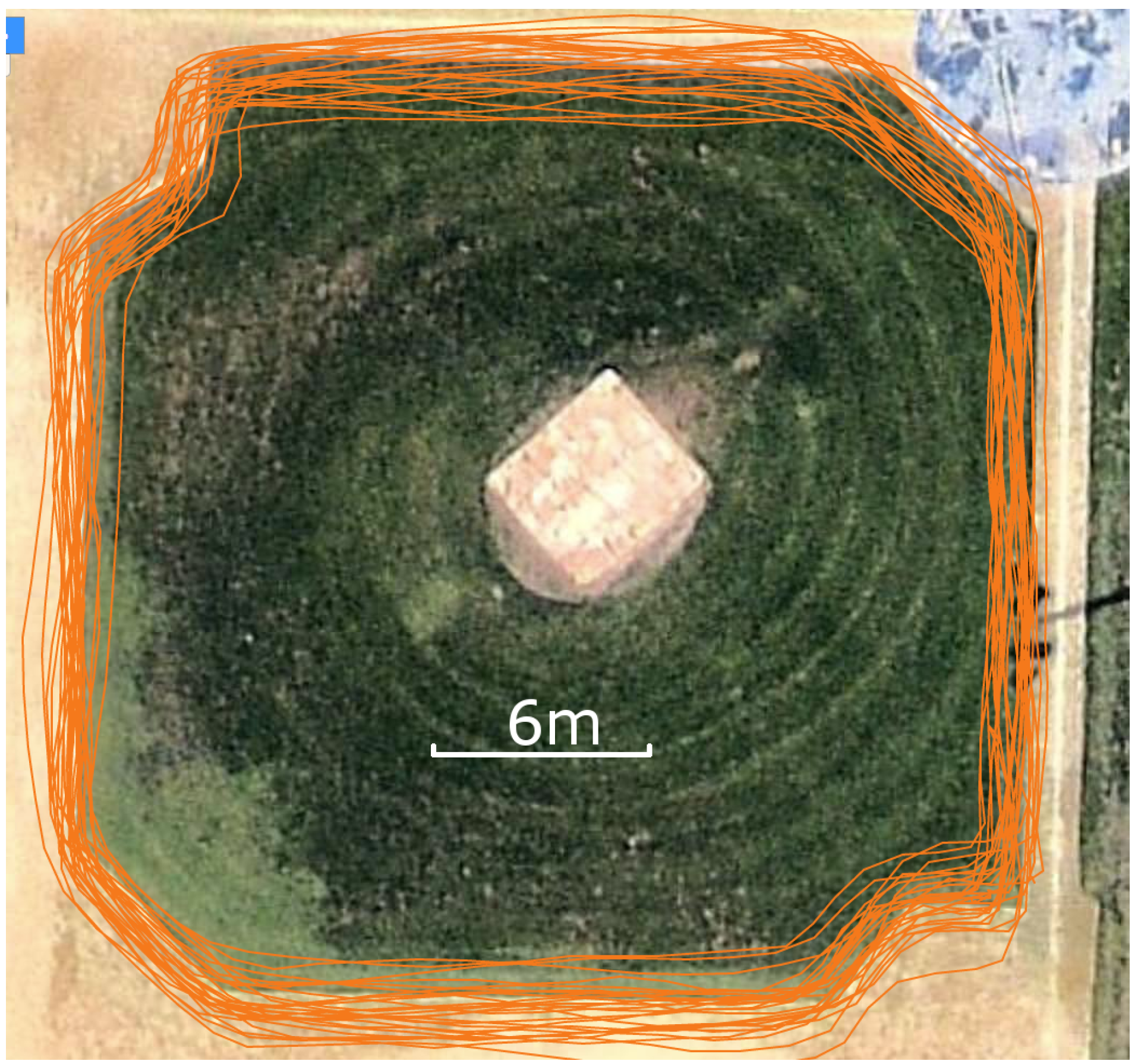
The aim of the final experiment was to assess the performance of the FAGPS approach for a moving target, as would be expected in a field robotics application. A base-ball diamond area was chosen as it has a well defined shape which varies in latitude and longitude. The start position (marked in Figure 5) was where the compensation on a geolocated point was performed. The experiment involved traversing around the edge of the grass in a clockwise direction as a speed of approximately 1.2 m/s. A total of 26 laps of the baseball diamond were performed over a period of 30 min.

5. Results and Discussion

This section provides the results and a discussion of the results for the simulation and each of the three experiments described in Section 4. These results demonstrate the feasibility of the proposed FAGPS scheme and the performance improvement over traditional non-corrected GPS receiver systems.

5.1. Simulation

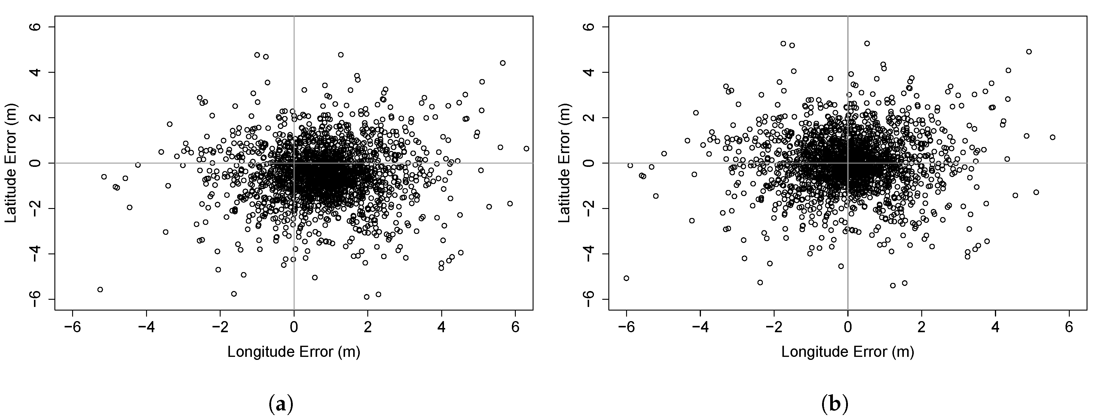
Figure 6a,b show the simulated error present for latitude and longitude for the non-FAGPS and FAGPS simulated data sets respectively. Visually it can be observed that although the datasets have a similar precision, the FAGPS dataset has significantly better accuracy.

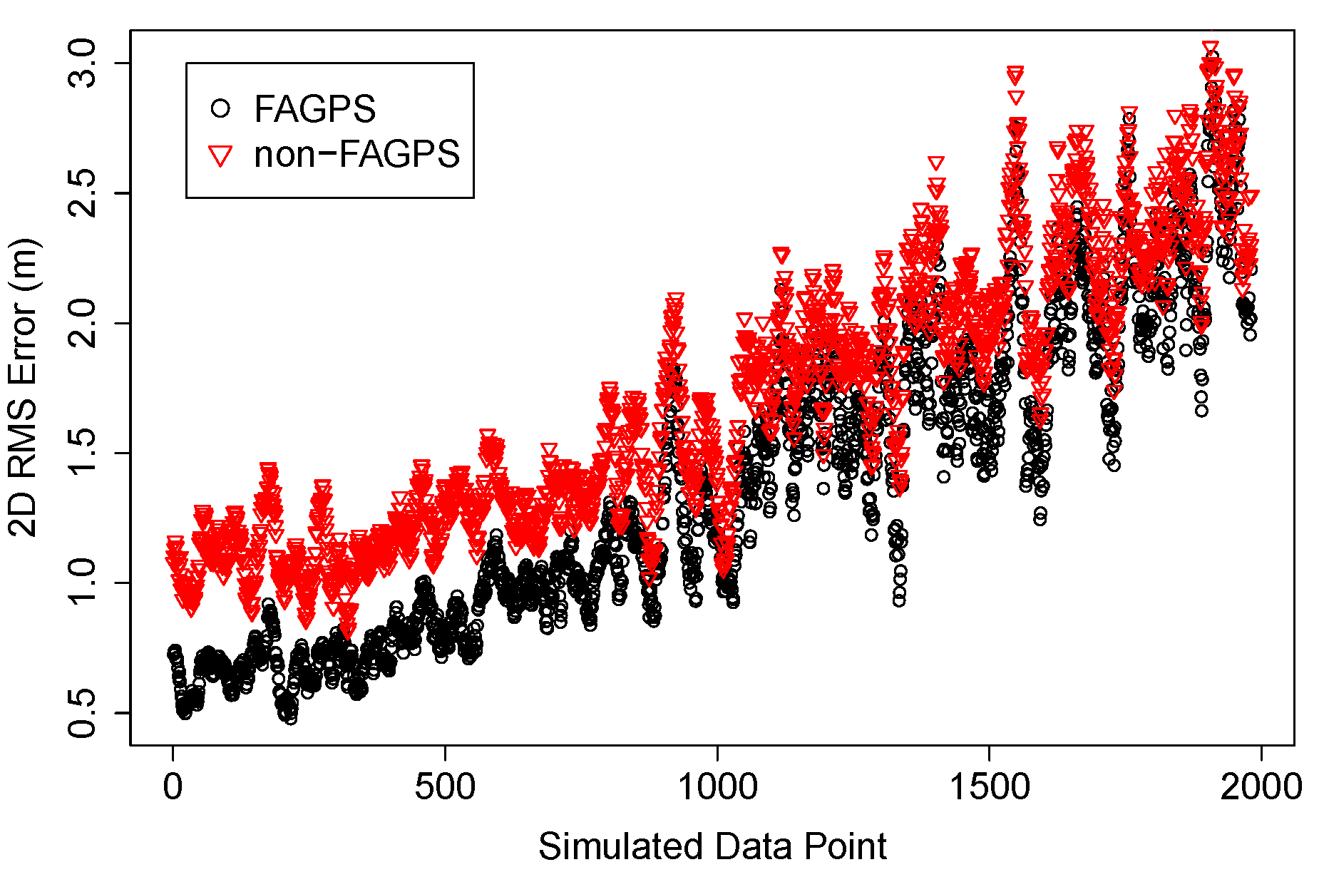
Figure 7 compares the 2D RMS error of the FAGPS and non-FAGPS schemes. It can be observed the in the short term the FAGPS performs with significantly lower error, due to the lower contribution from the time dependency in the additive noise. As the time dependent variable increases (above 1500 data points) the FAGPS scheme no-longer has an accuracy advantage. Reacquiring the fiducial marker and recalculating offsets would once again lower this time dependant noise and realise the accuracy advantage in the FAGPS scheme.

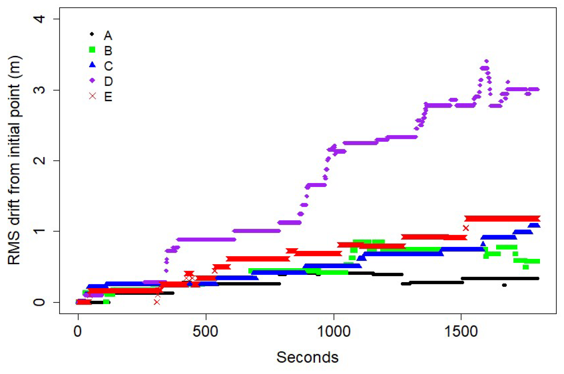
5.2. Results: Experiment 1

The drift in the results for the latitude, longitude and altitude is shown in Figure 8. This drift may initially seem very large, but it is taken over a period of over 44 h and is within the standard specified operational accuracy for traditional GPS systems.

The error over the 44 h test can be quantified using the 2DRMS error which is a way of expressing 2D GPS accuracy. 2DRMS is computed as double the square root of the average of the squared errors. For the 44 h test 2DRMS = 5.457 m.

Figure 9 shows 5 consecutive 30 min timeslots (each consisting of 1800 data points), demonstrating significantly smaller variance in position over the smaller time interval. The 2DRMS value for these 30 min sets is signficantly smaller than for the 44 h test as shown in

Table 3. Summary of horizontal error for different augmentation techniques.

Measurement	2DRMS (m)
A	0.45
B	0.83
C	0.73
D	2.99
E	1.28

.

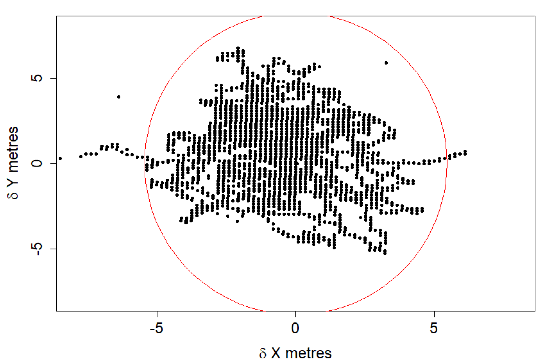
Figure 10 further shows the time dependence nature of the augmentation with significantly larger variance in error increasing over time. Figure 9 and Figure 10 seem to show error at discrete positions which highlights quantisation within the GPS receiver measurements (rather than presence of specific discrete errors).

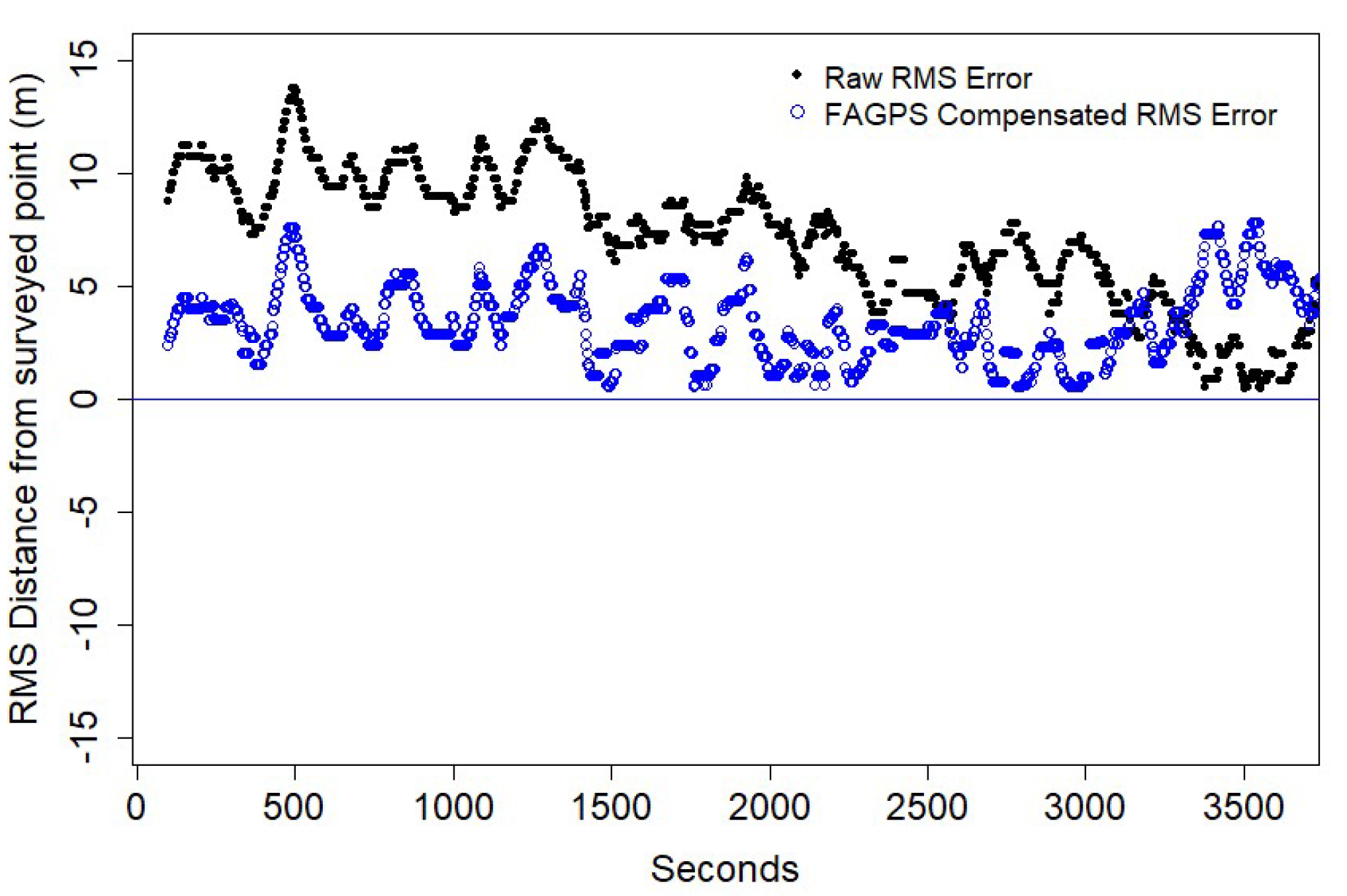
5.3. Results: Experiment 2

Figure 11 shows the horizontal RMS error of the raw GPS measurements in comparison to the FAGPS compensated measurements. The first 100 s have been excluded as these represented the time taken to move from PCM113580231 to PCM113580230. The first 30 min show a consistently smaller RMS error for the compensated data. Past the 30 min mark the compensated data provides less value in terms of increasing accuracy which we propose is due to the fact that the compensated values are time dependant and having aged are no longer accurate. This aging of the compensated values has several components including atmospheric conditions, potential multi-path effects and swapping between different satellites. At this point in time a fiducial marker could be reaquired to give a more accurate position estimation.

5.4. Results: Experiment 3

Figure 12 and Figure 13 show the results of experiment 3 with the RAW GPS data and the FAGPS compensated data respectively. The computed offsets were as follows: Latitude: 0.0000006667, Longitude: 0.0000140000. Given the relative size of each of the offsets the larger shift in the longitude compared to the latitude shown between the two figures is expected. The corrected values (Figure 13) although showing the same amount of fluctuation (in latitude and longitude) are clearly more closely aligned to the boarder of the grass.

6. Conclusions

This paper has proposed and demonstrated a GPS augmentation scheme, FAGPS, which uses geolocated fiducal images within an environment which can be observed and used to reduce GPS error (2DRMS error of 5.5 m to 2.99 m) for a period of 20–30 min. The FAGPS scheme has DGPS-like characteristics (in that local corrections are applied to GPS data to improve accuracy), the difference is that the same physical receiver is used to make the corrections. Although the accuracy doesn’t match that of DGPS, the cost of the system is orders of magnitude less than DGPS. DGPS operates on a much faster update rate than FAGPS (5 min compared to 20 min) which results in more up-to-date corrections being applied to GPS data.

The FAGPS scheme was assessed both through time-dependent simulations and fieldwork which demonstrate the improved short-term (15–20 min) accuracy by correction of initial GPS captured offset points. Future work is required to quantify the improvements that FAGPS could render for altitude and to validate the technique for flying vehicles.

References

- Kaplan, E.D.; Hegarty, C.J. Understanding GPS: Principles and Applications; Artech House: Norwood, MA, USA, 2005. [Google Scholar]
- National Coordination Office for Space-Based Positioning, Navigation, and Timing. Timing. 2014. Available online: http://www.gps.gov/applications/timing/ (accessed on 1 November 2019).
- Qi, N.; Xu, Y.; Chi, B.; Yu, X.; Zhang, X.; Wang, Z. A dual-channel GPS/Compass/Galileo/GLONASS reconfigurable GNSS receiver in 65 nm CMOS. In Proceedings of the Custom Integrated Circuits Conference (CICC), San Jose, CA, USA, 17 September 2011; pp. 1–4. [Google Scholar]
- Bajaj, R.; Ranaweera, S.L.; Agrawal, D.P. GPS: Location-tracking technology. Computer 2002, 35, 92–94. [Google Scholar] [CrossRef]
- DeCesare, N.J.; Squires, J.R.; Kolbe, J.A. Effect of forest canopy on GPS-based movement data. Wildl. Soc. Bull. 2005, 33, 935–941. [Google Scholar] [CrossRef]
- Wang, F.; Zhang, X.; Huang, J. Error analysis and accuracy assessment of GPS absolute velocity determination without SA. Geo Spat. Inf. Sci. 2008, 11, 133–138. [Google Scholar] [CrossRef]
- Braasch, M.S. Isolation of GPS multipath and receiver tracking errors. Navigation 1994, 41, 415–435. [Google Scholar] [CrossRef]
- Olynik, M.; Petovello, M.; Cannon, M.; Lachapelle, G. Temporal variability of GPS error sources and their effect on relative positioning accuracy. Paper Presented at the Institute of Navigation National Technical Meeting, San Diego, CA, USA, 28–30 January 2002. [Google Scholar]
- Djuknic, G.M.; Richton, R.E. Geolocation and assisted GPS. Computer 2001, 34, 123–125. [Google Scholar] [CrossRef]
- Monteiro, L.S.; Moore, T.; Hill, C. What is the accuracy of DGPS? J. Navig. 2005, 58, 207–225. [Google Scholar] [CrossRef]
- Morales, Y.; Tsubouchi, T. DGPS, RTK-GPS and StarFire DGPS performance under tree shading environments. In Proceedings of the 2007 IEEE International Conference on Integration Technology, Shenzhen, China, 20 August 2007; pp. 519–524. [Google Scholar]
- Zhang, N.; Wang, M.; Wang, N. Precision agriculture—A worldwide overview. Comput. Electron. Agric. 2002, 36, 113–132. [Google Scholar] [CrossRef]
- Fiala, M. Designing highly reliable fiducial markers. IEEE Trans. Pattern Anal. Mach. Intell. 2010, 32, 1317–1324. [Google Scholar] [CrossRef]
- Maurer, C.R.; Fitzpatrick, J.M.; Wang, M.Y.; Galloway, R.L.; Maciunas, R.J.; Allen, G.S. Registration of head volume images using implantable fiducial markers. IEEE Trans. Med Imaging 1997, 16, 447–462. [Google Scholar] [CrossRef]
- Abawi, D.F.; Bienwald, J.; Dorner, R. Accuracy in optical tracking with fiducial markers: An accuracy function for ARToolKit. In Proceedings of the IEEE/ACM International Symposium on Mixed and Augmented Reality, Arlington, VA, USA, 2–5 November 2004; pp. 260–261. [Google Scholar]
- Chen, T.Q.; Zhang, J.; Zhou, Y.; Murphey, Y.L. A smart machine vision system for PCB inspection. In Proceedings of the International Conference on Industrial, Engineering and Other Applications of Applied Intelligent Systems, Budapest, Hungary, 4–7 June 2001; pp. 513–518. [Google Scholar]
- Edwards, M.J.; Hayes, M.P.; Green, R.D. High-accuracy fiducial markers for ground truth. In Proceedings of the International Conference on Image and Vision Computing New Zealand (IVCNZ), Palmerston North, New Zealand, 21–22 November 2016; pp. 1–6. [Google Scholar] [CrossRef]
- Nguyen, P.H.; Kim, K.W.; Lee, Y.W.; Park, K.R. Remote marker-based tracking for UAV landing using visible-light camera sensor. Sensors 2017, 17, 1987. [Google Scholar] [CrossRef]
- Nahangi, M.; Heins, A.; McCabe, B.; Schoellig, A. Automated Localization of UAVs in GPS-Denied Indoor Construction Environments Using Fiducial Markers. In Proceedings of the International Symposium on Automation and Robotics in Construction, IAARC, Berlin, Germany, 20–25 July 2018; Volume 35, pp. 1–7. [Google Scholar]
- Diggelen, V.; Tromp, F.S. A-GPS: Assisted GPS, GNSS, and SBAS; Artech House: Norwood, MA, USA, 2009. [Google Scholar]
- Rohani, M.; Gingras, D.; Gruyer, D. A novel approach for improved vehicular positioning using cooperative map matching and dynamic base station DGPS concept. IEEE Trans. Intell. Transp. Syst. 2015, 17, 230–239. [Google Scholar] [CrossRef]
- Wullems, C.; Vasanta, H.; Looi, M.; Clark, A.J. A Broadcast Authentication and Integrity Augmentation for Trusted Differential GPS in Marine Navigation. In Proceedings of the Cryptographic Algorithms and Their Uses, Gold Coast, QLD, Australia, 5–6 July 2004. [Google Scholar]
- Soares, M.G.; Malheiro, B.; Restivo, F.J. An internet DGPS service for precise outdoor navigation. In Emerging Technologies and Factory Automation; IEEE: Piscataway, NJ, USA, 2003; pp. 512–518. [Google Scholar]
- Soares, M.G.; Malheiro, B.; Restivo, F.J. Evaluation of a Real Time DGPS Data Server; KU Leuven: Leuven, Belgium, 2004. [Google Scholar]
- Arnold, L.L.; Zandbergen, P.A. Positional accuracy of the wide area augmentation system in consumer-grade GPS units. Comput. Geosci. 2011, 37, 883–892. [Google Scholar] [CrossRef]
- Owen, C.B.; Xiao, F.; Middlin, P. What is the best fiducial? In Proceedings of the International Workshop on the Augmented Reality Toolkit, Darmstadt, Germany, 29 September 2002. [Google Scholar]
- Bruckstein, A.M.; Holt, R.J.; Huang, T.S.; Netravali, A.N. New devices for 3D pose estimation: Mantis eyes, Agam paintings, sundials, and other space fiducials. Int. J. Comput. Vis. 2000, 39, 131–139. [Google Scholar] [CrossRef]
- Claus, D.; Fitzgibbon, A.W. Reliable fiducial detection in natural scenes. In Computer Vision-ECCV 2004; Springer: Berlin/Heidelberg, Germany, 2004; pp. 469–480. [Google Scholar]
© 2019 by the authors. Licensee MDPI, Basel, Switzerland. This article is an open access article distributed under the terms and conditions of the Creative Commons Attribution (CC BY) license (http://creativecommons.org/licenses/by/4.0/).