1. Introduction and Motivation
Wireless Sensor Networks (WSN), commonly defined as the aggregation of small interconnected sensors capable of acquiring the status of their surrounding environment, have been used for many years. However, with the improvements both in hardware and communication technologies of the recent years, and the appearance of the Internet of Things, they are gaining popularity [
1]. Smart cities [
2,
3], smart buildings [
4], health-care systems [
5], industrial production, and many more fields are taking advantage of the data collection easiness that modern WSN offer to behave more efficiently. By collecting environmental data, smart buildings, for instance, can improve light and temperature control systems to save energy when possible, or even automate building actions by gathering people’s movements in order to increase their comfort [
6].
From an architectural point of view, a WSN includes one or more base stations (i.e., the sink nodes) and numerous nodes with sensing and forwarding capabilities (i.e., the sensors) distributed over a given area. The sensors can cooperate in order to relay data to the sink, possibly in a multi-hop manner. In this network, a careful determination of the data path between sensors and the sink is essential to ensure an efficient data delivery considering the specific constraints of a WSN such as energy, latency, bandwidth, transmission range, reliability, etc.
The essential and most important feature of a WSN is its availability for the longest possible time. However, providing exhaustive protection to all sensors against third-party attacks, natural risks or failure/out-of-battery issues can be economically and/or physically unviable in large WSN. Inadequate security can enable, for instance, Distributed Denial of Service (DDoS) attacks that can temporarily or permanently shut down a sensor or part of the network. Moreover, sensors can be incapacitated by unexpected natural conditions like earthquakes, massive rain, extreme heat or cold, etc.
Nonetheless, the availability of a WSN can be improved and still be economically viable if the protection is provided to a limited number of nodes. For this reason, in [
7], the concept of
criticality of a node has been introduced. The failure of a node for any possible reason (i.e., the node is not able to sense and forward any data anymore) has a specific degradation effect on the network performance: the higher the degradation, the highest the criticality of a node. According to this definition, the most critical sensor is, hence, the node that, if it fails, causes the highest deterioration on the network performance. Analogously, the two most critical nodes are the nodes that, if both concurrently fail, cause the highest deterioration, and so on. For instance, since the aim is to send the collected data from sensors through the network up to the base station, it is safe to say that sensors closer to the sink are probably holding more responsibility for such end. Thus, the incapacitation of these critical sensors can drastically hamper the correct functioning of the overall system, causing a higher performance degradation than the incapacitation of sensors located far from the sink.
Note that this definition varies from the general critical node definition adopted in literature [
8,
9,
10]; in that case, a critical node is a cut vertex, i.e., the incapacitation of such node breaks network connectivity and blocks data transmission. On the contrary, our definition can be considered a generalisation of it as it relays on the generic term of network performance. The network performance can be determined using one or more specific metrics like latency, available bandwidth, lifetime battery or connectivity. If the metric of interest is, for instance, the latency, the critical node is, therefore, the node that, once removed, causes the highest increase in the overall network latency. If the metric is the connectivity, then the critical node is a cut vertex as in the case of the definition commonly used in literature.
In summary, it can be seen that the identification of critical nodes and the evaluation of their impact in the WSN is important for the following reasons. Firstly, the provision of exhaustive protection to a given number of critical nodes can become viable. Secondly, the degradation that the WSN suffers when removing critical nodes is an upper bound; whatever node fails, its effect cannot exceed that degradation. Therefore, knowing this level of degradation is useful for the design and maintenance of the network and the adjustment of the service tolerance.
In this paper, we focus on two metrics for network performance, namely latency and lifetime. The former refers to the amount of time needed to transmit data from one sensor to the base station, and we assume in this work that it is directly related to the number of hops or jumps needed for that end. The latter expresses the amount of time elapsed until the first node battery runs out of energy and thus becomes unable to gather and transmit data. Such elapsed time is divided into time steps, each of which represents the creation and transmission of a single data packet per node. Moreover, nodes are not endowed with any additional power source generator, such as photovoltaic cells that could alter the calculations of lifetime.
In previous works, Mixed-Integer Programming (MIP) models have been proposed to identify the critical nodes and evaluate the degradation in terms of latency [
11] and lifetime [
7]. Although the MIP models provide exact results, they have two important limitations due to their complexity and long execution times required: (i) few critical nodes can be identified, and (ii) only WSNs with very limited number of sensors can be evaluated. In this paper, we propose a Greedy Randomised Adaptive Search Procedure (GRASP) meta-heuristic to overcome these limitations. The main contributions are:
A general framework for parallel GRASP execution;
A specific GRASP meta-heuristic to identify the critical nodes when the performance metric is the latency and evaluate their impacts;
A specific GRASP meta-heuristic to identify the critical nodes when the performance metric is the sensor lifetime and evaluate their impacts;
A comparison between the MIP and GRASP meta-heuristic results in WSNs with 100 nodes and one and two critical nodes;
An evaluation of the performance impact of one to five critical nodes in WSNs with up to 1000 nodes.
The rest of the paper is organised as follows.
Section 2 analyzes the state of the art. In
Section 3, we explain the current scenario and the motivation behind the creation of a GRASP meta-heuristic for solving bigger networks.
Section 4 defines the problem in detail. Then, in
Section 5, the GRASP meta-heuristic for both latency and lifetime models are presented, as well as the features used for reducing the number of criticality tests to perform. Finally, obtained results are shown in
Section 6.1 and
Section 6.2. Conclusions and future work are described in
Section 7.
2. Related Work
The problem of optimizing WSN in multi-hop networks has been widely addressed in many research articles. Among them, different network metrics such as latency and lifetime are usually used as the main parameters for optimization criteria. Moreover, Mixed Integer Programming models cover the majority of the evaluations thanks to its precision when delivering results.
For instance, in [
11], critical node removal impact in network latency is analyzed by means of an MIP model inserted into a framework that iteratively removes critical nodes one after the other. Latency is calculated as the overall sum of the number of hops needed to transmit data from each node up to the base station. Since the problem is formulated and solved using a MIP model, it is time-consuming to calculate simultaneous removals. Due to this, authors only calculate the impact of the first and second most critical nodes in randomly generated networks with up to 100 sensors distributed in a disk shaped area of 200 m radius.
Equally, The research in [
12] analyzes the same impact by using similar input data and system model layout but focusing on network lifetime this time. Even though the MIP models are very similar, authors here go beyond the threshold of [
11] by calculating the impact of up to five critical nodes in networks of 50 sensors with two different removal techniques: iteratively and simultaneously. In this case, lifetime is defined as the number of time slots needed until the first node runs out of battery life, taking into account that every node transmits one packet each time slot. Similarly, authors in [
7] deeply study the case of eliminating the node that offers more network degradation regarding latency. Results show the evolution of network degradation as the radius of the network decreases as well as when the number of nodes varies.
Another enhancement of the cited model is found in [
13], where authors merge both metrics, latency and lifetime, and evaluate the network degradation in lifetime when limiting the overall number of hops, i.e., when limiting maximum latency. Studied network sizes vary from 30 to up to 90 sensors.
Even though MIP models are very good at delivering exact results for many optimization criteria, they lack scalability. All the work cited beforehand share the same WSN structure: few network nodes and, overall, only the most and the two most critical nodes are studied.
In order to extend such scenarios, heuristics offer a good opportunity for obtaining close to optimal results in larger situations both in terms of network density and number of critical nodes. In this work, we try to cover this literature space that is yet to offer relevant results by presenting a GRASP meta-heuristic for networks up to 1000 nodes in a 630 radius area. These values are not arbitrary but scaled up from the base scenario of 100 nodes and 200 network radius presented in the aforementioned literature.
3. Current Scenario
As it has been previously said, we have studied the impact and identification of critical nodes in smaller networks with an MIP model capable of delivering exact results in terms of both latency and lifetime. Specifically, networks up to mica2 nodes and critical nodes subsets of have been studied. It has been decided to utilize mica2 motes as the basis of our study due to the amount of configurable transmission levels they enable.
It is worth mentioning that, in this scenario, the removal of critical nodes have been performed iteratively. That is, in the case of two critical nodes, the developed framework firstly computes and removes the most critical node and, then, from the remaining network, the second most influential critical node is identified and studied.
This decision has been taken due to the high complexity that exact models carry. MIP execution time for networks with sensors can take up to 2 min, versus the few seconds that GRASP offers. Moreover, when increasing the size of the problem both in terms of network sensors and number of critical nodes to identify, the inner exponential complexity of the MIP model makes it unfeasible for larger networks. For the creation of the GRASP, we have decided to take advantage of the reduction in complexity to modify our approach. One may think that the iterative removal of critical nodes covers enough scenarios that could happen in real systems. However, an even worse scenario could appear in which many critical nodes fail or are attacked at the exact same time. Imagine a system that has its nodes distributed across many buildings, with independent power sources. If critical nodes happen to be all inside the same building, a power outrage in such building could completely shut down the whole WSN. To solve this problem, instead of removing nodes one by one, GRASP identifies the set of nodes that, jointly, produce the most impact in the WSN. It is worth stating that, by the inner characteristics of heuristics, GRASP does not always offer the optimal solution. Instead, sometimes a local optimum is delivered as the best possible result. That is, while trying to improve the solution during the local search phase, it can happen that the explorable neighborhood does not improve the solution, and, thus, GRASP finalizes stuck in a local optima. To check whether our approach is good enough, an initial comparison between MIP results and GRASP results for small networks is shown.
4. Problem Statement
Given a WSN of
N mica2 nodes [
14], represented as
, a subset of critical node candidates
, the number of critical nodes to remove
C and a table
T shown in
Table 1 of the possible transmission levels and the energy needed to transmit at each of these levels, a solution is found when each node
i, apart from the Base Station and the critical nodes under testing, transmits to a node
j at a transmission level
k. Note that the chosen transmission level
k is the least possible level that permits the interconnection between sensor
i and
j range-wise, in order to reduce energy consumption levels at the minimum possible ones.
Therefore, a solution is represented by two vectors, namely
send and
key, both of size
N. The former stores, for each position
i, the node
j to which data are sent. Likewise, the later stores the transmission level
k needed for that communication. A solution is considered valid if
and
∖
:
Two different objective functions are considered, covering two of the major and most important requirements a WSN should have, latency and lifetime. The former makes reference to the required time to transmit data from one sensor to the sink node, whilst the latter refers to the amount of
time steps the network can be maintained alive without needing to charge or change node batteries if every node creates and transmits a single data packet at each aforementioned
time step. We consider network latency as the summation of the hops needed from each sensor to reach the base station, as shown in Equation (
1). The
calculatePathCost returns such value for a given node and a given network state.
Additionally, network lifetime is defined as the amount of packets that can be generated in each node until the critical one runs out of energy. It is worth noticing that this value is equal for all the nodes, and can be seen as the number of time slots
t that the network is alive if, at each time slot, one packet is generated and transmitted in each of the network nodes apart from the base station:
Equation (
2) shows a general definition for lifetime, where
battery is the amount of energy each node initially has,
and
are the values needed for receiving and transmitting a single packet, respectively, and
and
are the number of connections each node sends and transmits, respectively.
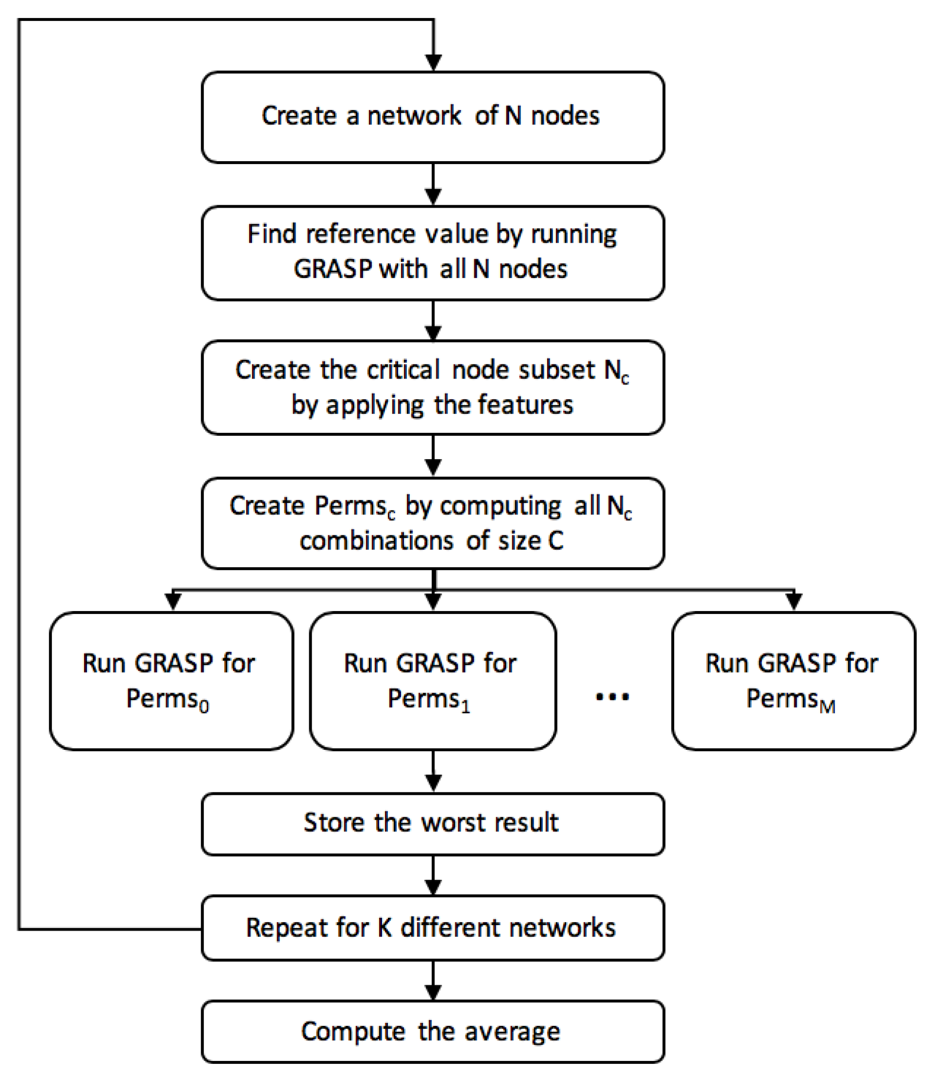
In order to find the most influential subset of critical nodes of size C, it is needed to calculate the impact of each possible subset formed by the candidates. That is, given , we compute all the possible combinations without order . Each of these combinations is then analyzed to see its impact in terms of the current objective function under testing. Once all the solutions are found, nodes pertaining to the combination with the worst solution are considered the critical nodes.
Figure 1 shows the framework used for such analysis. Firstly, a new network of
N nodes is created. This network is randomly generated by selecting
N node coordinates within the radius range under study.
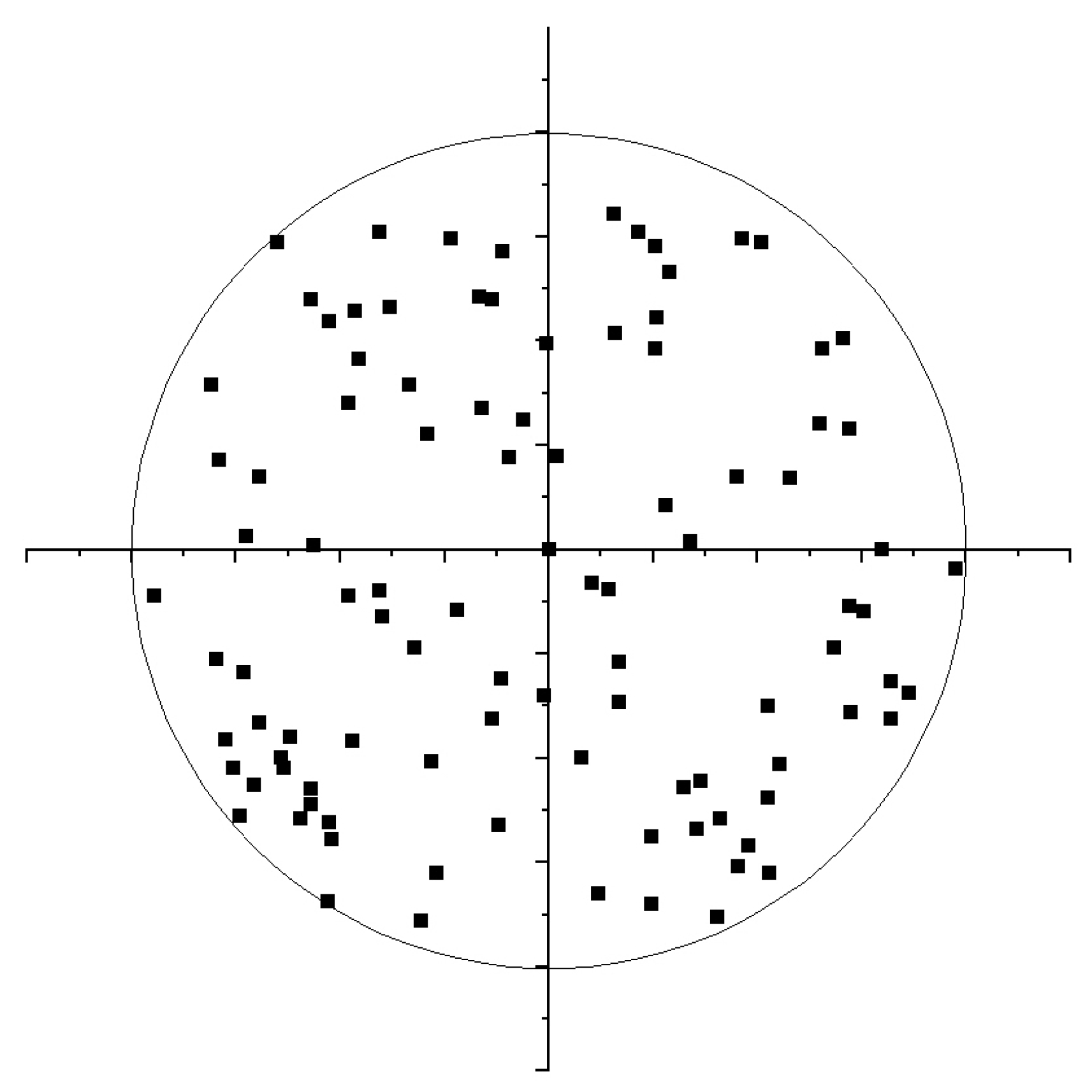
Figure 2 shows an example of a network of
sensors distributed across a disk shaped area of 200 m radius.
After that, we initially run the GRASP without removing any node to store the reference value. In the event of not finding a valid solution due to the randomness of the network generation tool, the network is re-generated. This process is done iteratively until a valid network is found.
Once it has finished, using the solution, we perform a node selection by means of features that are later explained. From the result set of nodes, all the combinations are calculated. Since our purpose is to analyze the impact of critical nodes when they are simultaneously removed, it is worth mentioning that the features are important to reduce the number of combinations and, thus, the complexity of the problem. For each of these combinations, a GRASP is run, and, as it can be seen in the figure, this is done in parallel. Once all the GRASPs have finished, the worst result is stored and a new network is analyzed. When finishing the K valid networks, the average and maximum values are stored as results.
5. GRASP
GRASP (Greedy Randomized Adaptive Search Procedure) is a meta-heuristic proposed by Feo and Resende [
15] for solving hard computational problems [
15]. The procedure is divided into two different phases, namely construction phase and search phase. In the former, a solution is greedily and iteratively constructed by adding one element to it until the size of the problem is reached. The latter phase is responsible for applying local search to the solution to try to improve it.
5.1. Latency GRASP
Algorithm 1 shows the generic code for the slightly tuned GRASP meta-heuristic used for the latency model. Regarding its input parameters,
contains the identification of the current nodes under a criticality test condition.
T makes reference to the table of relationships between each transmission range and the energy needed to transmit at that level, as shown in
Figure 1.
defines the number of iterations to perform before finishing.
is a mandatory GRASP parameter that controls the level of randomness to be applied when creating a solution. It has been finally decided to use an
for all the tests, since this value introduces a fair amount of randomness. Lower values might unable the GRASP to explore different neighborhoods due to starting most of the times from the same initial solution, and higher values might create bad initial solutions that the local search is then unable to properly improve.
Finally, G specifies a valid structure of a solution. As an output, the best solution found in terms of the current cost function being used is returned.
As for the actual code, line 2 contains the creation of an initial random solution to the problem. Then, this solution is improved by applying a local search algorithm as specified in line 3. Finally, if the cost of the new solution is better than the momentary best, the solution is updated.
| Algorithm 1 GRASP |
Require:
: subset of critical nodes to remove
T: transmission levels
α: randomness level specific for GRASP
G: node graph
Ensure:
: new node graph- 1:
while (MaxIter > 0) do - 2:
greedyRandomizedSolution() - 3:
localSearch() - 4:
if (cost() < cost()) then - 5:
- 6:
end if - 7:
MaxIter = MaxIter − 1 - 8:
end while - 9:
return
|
As it can be seen, in order to define the GRASP meta-heuristic, the greedy solution construction and the local search methods need to be defined. The following sections show both of these methods in more detail.
5.1.1. Construction Phase
During the first step of the GRASP, namely construction phase, a valid solution must be built. That is, interconnect all the network nodes with valid transmission paths according to the transmission levels shown in
Table 1 until every node is capable of reaching the sink node. Algorithm 2 shows the code of the method responsible for such matter. Starting from an empty set as shown in line 1, we define a loop in lines 2–16 in which each iteration is responsible for adding a new node to the solution until the size of the problem is reached. To decide which node to include in the current step, firstly the cost of adding each node outside both the partial solution and the critical nodes subset
is computed as seen in lines 4–6. When all the costs are calculated, a Restricted Candidate List (RCL) is built by adding only the nodes with a cost inside the range [
,
* (
−
)] (lines 10–14). These thresholds represent the minimum and the maximum
adding cost for the nodes yet outside the solution. To finalize, a random node is extracted from the RCL and added to the solution.
The objective function of the problem is defined inside the function responsible for calculating the cost of adding an element to the current solution, as seen in line 5.
| Algorithm 2 greedyRandomizedSolution |
Require:
α: randomness level specific for GRASP
Ensure:
G: node graph- 1:
- 2:
while ( < problemSize) do - 3:
- 4:
for and do - 5:
costOfAdding(, G) - 6:
end for - 7:
- 8:
minCost() - 9:
maxCost() - 10:
for do - 11:
if () then - 12:
- 13:
end if - 14:
end for - 15:
selectRamdonNode() - 16:
end while - 17:
returnG
|
In this construction phase, there is no order in which nodes are added to the solution, or a global condition to test if the insertion is the best possible one. This is why the method is considered greedy because, in each step, the best local cost is chosen as a candidate.
5.1.2. Search Phase
The second or search phase of the GRASP algorithm is responsible for improving, if possible, the solution created by the construction phase. In order to do so, the search explores the solution neighborhood to check if there are any with better cost in terms of the objective function under use.
Algorithm 3 shows the code for the local search. Regarding its parameters, contains the solution to be improved, and specifies the value of the stopping criteria. It limits the number of consecutive iterations to perform without solution improvement. Once this threshold is reached, we consider that contains the local best.
For improving the solution, the algorithm firstly gets a random node n from the solution. Then, it computes the current cost of sending data through its path until reaching the base station. Since this path has been greedily selected by the constructive phase, we check whether there are alternative paths through any of the neighbors of n ending at the base station that have better cost. If so, the path is updated and the local search continues. In addition, the consecutive iterations without improvement are reset.
| Algorithm 3 localSearch |
Require:
: current solution
: maximum number of consecutive iterations to perform without improvement
Ensure:
: improved solution- 1:
- 2:
whiledo - 3:
n = getRandomNode() - 4:
= calculatePathCost() - 5:
for Neighbours(n) do - 6:
= cost() + calculatePathCost() - 7:
update() - 8:
if then - 9:
- 10:
- 11:
end if - 12:
end for - 13:
- 14:
end while - 15:
return
|
5.2. Lifetime GRASP
The lifetime GRASP code is very similar to the latency one presented in
Section 5.1 thanks to the inner characteristics of the meta-heuristics, which deliver a structure that needs very small tuning for solving different problems.
The outer GRASP code presented in Algorithm 1 is valid for the lifetime model since it also needs the critical node subset in each execution to check the one with more lifetime impact. Moreover, the greedy randomized method previously presented can also be re-utilized. In the case of the local search, major changes have been performed in order to correctly explore the neighborhood and improve the solution as much as possible.
The following sections explain more in detail each of the methods and the new decisions taken.
5.2.1. Construction Phase
As it has been said, the construction phase for the lifetime model follows the exact same approach as the latency model. Algorithm 2 is, therefore, also valid for this model. The reason behind such decision relies on the fact that the more hops a solution contains, the more energy is consumed and, thus, the lifetime is not as high as it could have possibly been. For calculating the overall network lifetime, let us consider a node
i, with maximum battery capacity of
. Let
be the amount of connections that node
i redirects to node
j. Since every node only generates its own connection, it can be rapidly seen that
is the amount of connections that node
i receives. The following formula calculates the lifetime, or amount of time steps
t that node
n can hold up without rendering out of energy:
where
stands for the amount of energy needed for receiving one packet and
makes a reference to the amount of energy needed to transmit from node
i to node
j according to their distance, as specified in
Table 1.
The formula is divided into two parts: energy needed to receive and energy needed to retransmit. Since the energy needed to receive can be seen as an overhead, we concluded that a network with minimum hop count holds the lowest possible retransmissions and thus the additional overhead paid for having to receive packets is minimal. In some cases, this statement could be wrong: according to the energy and range values seen in
Table 1, in very specific scenarios, it can be calculated that the amount of energy for doing two hops plus the energy needed to receive allows the network to reach the same distance with lower energy consumption than one single hop. However, this constructive algorithm provides a very good starting point and the local search is responsible for improving it by correcting such scenarios.
The overall network lifetime is the minimum among all the node lifetimes since this value represents the amount of time steps until the first node exhausts its battery.
5.2.2. Search Phase
Search phase for the lifetime model follows the same pattern as the latency one, but with completely different swapping criteria. Algorithm 4 shows the method responsible for improving the input solution. As it can be seen, the parameters are exactly the same as before, being a valid constructed solution and the maximum number of iterations without improvement until the search finishes.
| Algorithm 4 localSearch |
Require:
: current solution
: maximum number of consecutive iterations to perform without improvement
Ensure:
: improved solution- 1:
- 2:
whiledo - 3:
c = getCongestedNode() - 4:
n = getRandomLeaf() - 5:
= calculateMaxLifetime() - 6:
for Neighbours(n) do - 7:
if changeIsPossible() then - 8:
makeChange() - 9:
= calculateMaxLifetime() - 10:
if then - 11:
- 12:
end if - 13:
end if - 14:
end for - 15:
- 16:
end while - 17:
return
|
Due to the heterogeneity on the energy needed to transmit depending on the range and the different relay that each network node holds, it is safe to say that there will be a node or a group of nodes restricting the lifetime. Then, the local search is responsible for finding the congested nodes and balancing their load in order to increase the overall network lifetime. To do so, we firstly identify the more congested node c. In order to reduce its load, we randomly select one node n sending data to such congested node c. Then, we try to redirect the connectivity of n to another of its neighbors different from c so that the network load is more distributed and the lifetime can be increased. To avoid making changes with which the lifetime is not increased, we only mark the current change as possible if the lifetime l can be increased at least to . If the conditions are met, the network is updated for the following iteration.
5.3. Feature Selection
Given a WSN with N nodes, it is safe to say that node importance inside such network significantly varies from one to another. Since all the nodes must finally transmit their data to the sink node (i.e., base station), it can be seen that the furthest nodes will act as leaves by only sending data, without needing to retransmit another node’s packets. However, nodes very close to the base station will most likely act as bridge nodes, retransmitting the data from the rest of the nodes that are unable to reach the base station by themselves. Having this in mind, we have defined three features that allow us to rank the importance of the nodes in order to reduce the number of criticality tests. These features are the following:
Connectivity: Given a node
, node connectivity is defined as
where
refers to the maximum possible range that a node can transmit using the more costly transmission level shown in
Table 1.
Hops to base station: For a node
i, this feature is defined, as its name indicates, as
, where
bs stands for base station and
refers to the maximum possible range that a node can transmit using the more costly transmission level shown in
Table 1.
These two initial features can be calculated prior to obtaining any solution for a given network, since the only requirement for calculating them is the distance between nodes, which can be extracted from the node coordinates. However, we also define another feature directly related to the solution of the base case scenario (i.e., when no critical nodes are removed from the network):
Relay: A node i defines its relay as the number of outgoing connections. This number is equal to the amount of ingoing connections plus its own generated ones. Given the solution matrix f and the value which indicates how much data node i sends to node j, the relay for node i is defined as .
Once all the features are defined, it is needed to see whether their use actually allows us to reduce the number of nodes to test for criticality without losing precision in the solution. In order to do so, 10 network topologies of
nodes are created by using a random node distribution in a 200 m radius area. These topologies are then analyzed using the GRASP meta-heuristic presented in
Section 5.1 for obtaining the identification of the critical nodes by testing all the possible nodes and subset of nodes for both the latency and the lifetime model. Once the critical nodes are identified, we search their ranking position in the three features. It is worth mentioning that the nodes pinpointed as critical may actually not be the correct ones obtained by the analogous MIP model. However, we firstly analyze the features by only checking the GRASP, and, in
Section 6, we analyze the percentage of identification success.
Table 2 and
Table 3 show the overall percentage of success for each critical node subset tested and different individual feature thresholds for the latency and the lifetime models, respectively. Specifically, the top 3, 5, and 10 are used for both connectivity and relay. The hops to base station, however, differ from the two tests: in the case of the latency, it is sufficient to have
in order to achieve a
success. The lifetime model needs to extend this range up to
to achieve the same result.
As it can be seen, the hops feature is a really good critical node predictor, since all the critical nodes are always very close to the base station. Relay is also a good predictor, since the values obtained for the top 10 are very high in both scenarios. However, connectivity does not seem to offer good reliability to identify critical nodes.
With these results, it is clearly seen that enforcing high rank in all the features to a node in order to include it in the critical node subset is not reliable and the percentage of success will be very low. Similarly, one may think that testing all the nodes with for the latency or for the lifetime will be the most reliable scenarios. Nevertheless, by only restricting such feature, the number of nodes for testing is, on average, still very high to obtain plausible times when running GRASP for larger networks and larger subsets of critical nodes.
For all of this, it has been decided to enforce a membership of two out of the three features, independently of the combination, to consider a node plausible for criticality testing.
Table 4 and
Table 5 show the results of such scenarios. As it can be seen, the identification of the most critical node increases when increasing the top threshold, and it arrives to
when the
top 10 is used. In the case of two critical nodes, the percentages generally decrease. However, using the same
top 10 threshold, the success rate is considerably high (
) for the latency, and achieves a
success rate in the case of the lifetime.
In conclusion, features are a good tool for reducing the complexity of the problem by selecting only candidates with high possibility of being critical instead of testing every single network node. Results presented in
Section 6 are extracted by utilizing such features. If nothing is indicated, results are extracted using
top 10 for both connectivity and relay, whilst
is used for hops to base station in both models, in order to maintain consistency.
6. Results
This section presents the results obtained for both the latency and the lifetime models by initially comparing the MIP results obtained for small networks with the GRASP meta-heuristic ones. After that, results for bigger networks are presented. All the calculations have been performed using a MacBook Pro early 2015 (Apple, Cupertino, CA, USA) with a 2.7 GHz Intel Core i5 processor (Santa Clara, CA, USA) and 8 GB 1867 MHz DDR3 memory.
The initial MIP and GRASP comparison results are obtained by studying 10 networks of nodes evenly distributed in a 200 m radius area. For each of these networks, we show the latency and lifetime values for both methods as well as the nodes pinpointed as critical. Such metrics allow us to conclude whether the effectiveness of the GRASP is good enough.
The study of larger networks has been initially performed with the same 200 m radius area for even node distribution. For , results are shown for up to five simultaneous critical node removals. In the case of , results are reduced to four critical nodes. Finally, for , the three most influential nodes are calculated.
Networks with more node density have not been studied because of the already small values obtained during the aforementioned tests, and, since GRASP is not an exact tool, it is difficult to extract correct conclusions with such little margin error. Moreover, the limitation in the area to deploy the sensors highly increases the complexity of the problem due to the amount of neighbors each node can send data to, increasing the explorable neighborhood during construction and search phases.
For all that, it has been decided to scale the
and 200 m radius network in order to study larger ones with the same node density. Moreover, the
hops to base station threshold feature is tuned to also consider this scaling.
Table 6 shows the radius and hops to base station thresholds used for networks with
nodes. The rest of the feature thresholds remain the same. Since these new networks share the same characteristics in terms of node density and feature thresholds, but, scaled up, we want to see whether the impact of critical nodes also remains the same. The decision for not studying more critical node impact relies in the trade-off between the time needed for finding the solution and the network degradation variation.
Table 7 shows a comparison between the MIP and GRASP execution times needed for selecting the most critical node in a network of
nodes. As it can be seen, the difference in time is substantial for such small networks. When increasing the network size, not only the complexity of the problem increases, but also the number of iterations to perform. That is, for a network of
sensors, it is needed to execute the MIP model
N times in order to find the most critical node. For this, and, due to the inner high exponential complexity that MIP presents versus the one that GRASP offers, it has been decided to develop the meta-heuristic for obtaining results for bigger networks and a wider set of critical nodes.
6.1. Latency Results
Table 8 shows, for the 10 different network topologies studied, the latency value obtained both in the MIP model and in the GRASP, as well as their percentage difference. Moreover, the table also shows the identifier of the nodes pinpointed as critical. As it can be seen, each case is summarised into two rows: the first one shows the results of one critical node removal, whilst the second one shows two critical nodes removal results. As previously stated, the critical nodes in the MIP model are iteratively extracted, and, for this reason, each table row only shows the current node removed. For the case of the GRASP, both tests are independent and, thus, complete results are shown for one critical node and two critical nodes’ removal.
Regarding the identification of the critical nodes, GRASP offers really good results when extracting the most influential node, delivering a 90% success rate. However, when testing the network for two critical nodes, this rate is reduced to around 65% due to the GRASP failing to identify one or both of the critical nodes. The justification of such low value lies in the fact that MIP and GRASP tests for this scenario slightly differ. Since GRASP nodes are being removed simultaneously instead of iteratively, there might be a combination of two nodes that deteriorates the network more than the iterative removal of the two most influential ones.
Network #8 is further analyzed in order to understand why the first critical node is missed. The first important aspect to notice is that the missed and the correct critical nodes are inside the critical node test set selected by the features. Specifically, both are in range of the base station and their neighborhood is inside the top 10. Regarding the solution obtained by GRASP, the relay of both nodes slightly differ. However, it can be seen that both send data directly to the base station. The MIP results deliver the same scenario, but, in this case, the relay is very similar between them.
After seeing that the characteristics of the missed and the critical nodes are almost identical, a conclusion can be extracted by looking at the latency results. The difference of the MIP latency values obtained for the two nodes is minimal, making it difficult for the GRASP to actually find the optimal value, and, instead, obtaining a slightly worse one with a different node pinpointed as critical.
Figure 3a depicts the results of the previously explained tests in which node density is increased by adding more nodes to the same network deployment area. Each of the lines drawn A–
C shows the average impact when removing the most
C critical nodes from the network.
There are two main conclusions that can be extracted. Firstly, it can be clearly seen that, as the number of nodes inside the network increases, its deterioration when removing a fixed quantity of critical nodes decreases. As there are more nodes inside the network, the paths to which a node can transmit increase, the connections between the nodes are more distributed and, thus, network flexibility increases, reducing the impact of critical node removal. Specifically, it can be seen that latency deterioration in 500 node networks is half that of 100 node networks.
Secondly, when looking at the values of a single network size, it can be seen that the removal of more critical nodes has higher impact on the latency increment. The theory behind such result is the following: let c be the critical node removed and the nodes that send data to it. When c is removed, latency is reduced by the amount of hops c needs to send data to base station, but, at the same time, it increases by at least since the new path for such nodes will be at minimum one hop larger. If it happens to be a faster path, it would have been selected either during the construction or search phase. This explanation is not true when c shares two paths with the exact same length or the network does not have inner nodes. However, such scenarios are very specific and only possible in networks with very few nodes, which is not the case. The explanation is also extensible when more than one critical node is removed. It is worth mentioning that these are theoretical calculations and they might slightly differ from the obtained results in some cases due to the inexactitudes of the GRASP meta-heuristic.
Additionally, in order to clearly see how much impact the removal of
C critical nodes can have in a network, the maximum values are shown in
Figure 3b. Even though the tendency of the curves remains almost the same as before, the latency increment is much higher, arriving to double the average in some cases.
Figure 3c,d show, respectively, the average and maximum execution time needed for calculating the previous values. As it can be seen, the time needed to remove a fixed amount of critical nodes increases exponentially with the number of nodes, mainly due to the amount of neighborhood checks to perform. Moreover, when looking at a fixed network size, it can also be seen that the tendency when removing a higher amount of critical nodes is exponential because of the combinatorial factor introduced for calculating all possible combinations of critical nodes’ subsets.
Figure 4a shows the average results after scaling the
node network deployed within a 200 m radius area. Performing a scaling to keep the same characteristics as the
and 200 m radius network allows us to conclude that the latency deterioration remains the same, with very small variation, when removing the same amount of critical nodes.
However, when looking at the maximum results in
Figure 4b, the horizontal tendency disappears. Even though the average is maintained, it can be seen that the worst scenarios can have huge deterioration variations. For instance, the worst network of
nodes increases its latency by
when removing more than four critical nodes, and this percentage is drastically reduced to around
for the
network. These results are representative of the network space studied, and, since these values are the worst cases, the study of more networks could possibly change them. However, due to the number of nodes and distribution areas, it is impossible to cover all possible scenarios.
Even though scaled networks perform differently in terms of latency deterioration, the exponential trend in the execution time remains the same as shown in
Figure 4c,d.
6.2. Lifetime Results
Equal to the latency model, the comparison between the MIP model and the GRASP meta-heuristic for small networks of
nodes distributed in a 200 m radius area are firstly presented. These results allow us to appreciate the margin error that the GRASP presents. Moreover, it can be checked whether GRASP ensures a correct critical node identification.
Table 9 shows such results. Each network is represented by two rows: the first one makes reference to the one critical node removal test, whilst the second one stands for the case where two critical nodes are removed. It is worth remembering that the MIP iteratively deletes the critical nodes, whilst the GRASP does it simultaneously.
Table 9 shows the comparison between the MIP model and the GRASP results, as well as the critical nodes’ identifiers. The lifetime values shown express, as previously explained, the
time slots the network can be maintained fully operative if every node generates and sends one packet in each of these
time slots.
In this case, the difference between the MIP and the GRASP substantially differs. Thanks to the exactness of the MIP, node transmissions are split between different nodes instead of sending all the data to a single one. However, due to the approximation behavior of GRASP, the split of the transmissions cannot be exactly performed. As it can be seen, GRASP lifetime is 18% less for the one critical node removal case, and it increases to around 22% for the two critical nodes one. Looking at the networks independently, it can be seen that, in some cases, GRASP almost reaches the best value given by the MIP model.
Critical node identification also suffers a degradation compared to the latency model. When removing the most critical network node, success rate is lowered to 80%, mainly due to the efficient transmission split that MIP performs. In the case of two critical nodes removal, the difference in node removal procedure also lowers the success rate to 60%.
Networks #5 and #7 have been further analyzed in order to understand why the first critical node is not correctly pinpointed. By looking at the feature rank and individual results that both the MIP and the GRASP deliver for the correct and the missed nodes, it can be clearly seen that such nodes share many similarities, their constant appearance in the critical node test set being the first and most important one.
In the case of network #5, the missed and the correct critical nodes are within reach of the base station, with an extensive neighborhood. Regarding the relay feature, the MIP grants both nodes a very similar value, among the top ones, and the GRASP assigns the same relay value. Equal to the latency case mentioned before, the similarity in the final MIP lifetime value makes it difficult for the GRASP to properly find the optimal value.
Network #7 shares many similarities with the aforementioned network #5. Equally, the missed and the correct critical nodes are in the range of the base station, and they both send data to it. Moreover, their neighborhood is among the top 10. Moreover, the MIP relay values are almost identical between the two nodes, being identical in the case of the GRASP. Final lifetime values only differ by a single unit in the case of the MIP. For such reason, it is very difficult for the GRASP to reach the optimal scenario.
In conclusion, even though the success rate for the first critical node is not 100%, it can be seen that the missed cases can also be useful for understanding the characteristics of the network and the critical nodes.
Figure 5a shows the results for the tests in which node density is increased. Each of the lines A–
C shows the average impact when removing the most
C critical nodes from the network. As it can be seen, the behavior of the previous average latency increase results and the current average lifetime decrease share many similarities. Firstly, as the number of nodes inside the network increases, the degradation in the lifetime lowers, mainly due to the flexibility that dense networks offer in terms of available paths for distributing the data delivery. Second, and most importantly, it can be seen that, if nodes inside the network share the same battery capacity, the lifetime decreases as the number of critical nodes removed increases. When a critical node
n is removed, the network slightly loses flexibility, and paths crossing
n need to be redirected to a more costly destination, reducing the lifetime of those nodes and thus the overall network lifetime.
Figure 5b extends the previous results by showing, in this case, the maximum lifetime decrease values obtained. It is worth noticing that, although the decreasing tendency is slightly maintained, the smoothness of the curve previously seen disappears. Again, these results are only representative of the network space tested, and the study of different network layouts may vary the maximum results. However, it is not possible to study every single network due to the amount of possibilities.
Average and maximum execution times are respectively shown in
Figure 5c,d. Both plots show the exact same exponential tendency. However, maximum values are much higher, arriving to double the average in some cases.
Results for lifetime in scaled networks are presented in
Figure 6. Similar to the latency model, the horizontal tendency appears as shown in
Figure 6a. However, in this case, the variations between different network sizes are more considerable, but it can be concluded that the lifetime decrease is maintained when the network is scaled up. Nonetheless, when looking at the maximum decrease values in
Figure 6b, instead of a horizontal tendency, a slight increase is seen.
Figure 5d shows the average execution time for the lifetime decrease model. The exponential tendency is clearly seen for the AV-2, AV-3 and AV-4 cases. Equally, in the case of maximum execution times depicted in
Figure 6d, this exponential tendency continues but with bigger time values, arriving to more than 2 h in some cases.
7. Conclusions and Future Work
In this work, we have extended the results obtained by the MIP model previously presented thanks to a GRASP meta-heuristic capable of handling larger networks in terms of nodes and also larger tests in terms of number of critical nodes. Moreover, the decision of simultaneously removing such critical nodes instead of doing it iteratively has driven us to the following conclusions:
The simultaneous removal allows for covering the worst possible scenario, in which part of the network unexpectedly shuts down and many critical nodes are disabled at the same time. An IoT system distributed across many buildings or zones can have part of the network disabled due to natural disasters, malicious attacks or power outages. On the contrary, individual sensor incapacity is less likely to happen due to the possibility to monitor and prevent unwanted battery levels or sensor behaviors prior to the actual failure.
In many cases, the iterative and simultaneous cases end up identifying the same nodes as critical. This means that if, for any reason such as time limitation or computational power, it is not possible to cover the simultaneous case, by computing the iterative scenario, it is enough to identify the most disruptive nodes with sufficient certainty. However, this should not be the common proceeding.
Nonetheless, by looking at the results presented, we can appreciate that the identification of critical nodes is crucial to deliver good service even when the network is being disrupted. Although their impact on fixed deployment areas decreases as the number of nodes increases, their failure is still relevant enough to consider securing their integrity. Moreover, as deployment area scales, the impact of the critical nodes remains almost equal, contradicting the idea that, since there are more nodes, their importance should be lower as the number of nodes increases. Because of that, it is clear that the security and reliability of the most influential nodes is very important to avoid the shut-down of a whole system network, which can induce large economic losses for a company that deeply relies on gathered data to acquire benefits or perform its duty correctly.
Additionally, even though the meta-heuristics do not deliver an exact and correct result all the times, the success rate obtained offers a good opportunity for large scale scenarios in which exact optimization tools are unable to handle such amount of data.


