Integrated Predictor Based on Decomposition Mechanism for PM2.5 Long-Term Prediction

Featured Application

This work can be used in the intelligent system for the smart city, smart agriculture, etc.

Abstract

It is crucial to predict PM2.5 concentration for early warning regarding and the control of air pollution. However, accurate PM2.5 prediction has been challenging, especially in long-term prediction. PM2.5 monitoring data comprise a complex time series that contains multiple components with different characteristics; therefore, it is difficult to obtain an accurate prediction by a single model. In this study, an integrated predictor is proposed, in which the original data are decomposed into three components, that is, trend, period, and residual components, and then different sub-predictors including autoregressive integrated moving average (ARIMA) and two gated recurrent units are used to separately predict the different components. Finally, all the predictions from the sub-predictors are combined in fusion node to obtain the final prediction for the original data. The results of predicting the PM2.5 time series for Beijing, China showed that the proposed predictor can effectively improve prediction accuracy for long-term prediction.

1. Introduction

Air quality has had a huge impact on human health and climate, so the effective management of air quality and its accurate assessment and prediction have received widespread attention in recent years. As one of the important air quality indices (AQIs), the prediction of PM2.5 concentration is a necessary evaluation parameter for air quality forecast [1,2]. It is difficult to obtain an accurate long-term prediction of PM2.5 concentration because PM2.5 comprises typical complex nonlinear time-series data [3], where the vector field of state dynamics is a nonlinear function of state variables. In the literature, the estimation and prediction of air quality are often based on mathematical models, the predicted models can be established through some parameter estimation methods [4,5,6,7], some have used input-output representations [8,9,10,11], and others have used state-space models [12,13].

The methods used to realize accurate and efficient prediction of complex time-series data include traditional time-series modeling methods, shallow networks based on machine learning, and deep-learning networks. Traditional methods predict the future trend of PM2.5 based on a statistical model of historical data including autoregressive-integrated moving average (ARIMA) models [14] and vector auto-regression (VAR) [15]. ARIMA is a linear modeling method that provides accurate predictions for approximate linear relationships. However, its prediction performance is not good enough for nonlinear prediction problems.

To capture the complex nonlinearity of PM2.5, a back propagation (BP) neural network has been widely applied in time-series data prediction [16,17,18]. Other shallow nonlinear networks based on a machine-learning mechanism such as the improved gray neural network model [19] and the radial basis function (RBF) neural network [20] have also been used to predict time-series data. Xu et al. [3] proposed a supplementary leaky integrator echo state network (SLI-ESN), which added the historical state term of the historical moment to the calculation of a leaky integrator reservoir. Compared with an echo state network (ESN), a leaky integrator ESN (LI-ESN), an extreme learning machine (ELM), a hierarchical ELM (H-ELM), a stacked auto-encoder (SAE), and a traditional SLI-ESN, the proposed SLI-ESN of Xu et al. [3] could achieve good prediction results, but its long-term predictions were not satisfactory.

As a shallow network still cannot effectively extract the complex nonlinearity of the data, decomposition must be used; that is, the data must be decomposed into multiple components to reduce its complexity, and then multiple sub-models are used to improve the prediction performance. For example, García et al. [21] decomposed a long-term data series into smaller seasonal component patterns. Jesús et al. [22] divided a pollen-concentration data series into seasonal and random parts, used partial least-squares regression (PLSR) to fit the residuals, and established an airborne pollen time-series model to predict the daily pollen concentration. Ming et al. [23] extracted accurate seasonal signals, and used maximum likelihood estimation (MLE) to estimate the long-term trend of the seasonally adjusted time series, which improved the prediction accuracy of the data. We note that the use of these decomposition methods compensates the nonlinear modeling capabilities of shallow networks. The original time-series data are decomposed into multiple sub-sequences, and the degree of nonlinearity of each sub-sequence is reduced. Therefore, for each sub-sequence, the training process of shallow network parameters is easier to converge, and the loss function of the training is smaller, so the obtained model is more accurate, and the prediction performance improved.

To improve the ability to model nonlinearities, deep neural networks have made great progress in regression prediction in recent years, especially the regression deep-learning network represented by a recurrent neural network (RNN) [24]. However, the RNN structure encounters gradient disappearance and gradient explosion during network training, and it is difficult to perform multi-step optimization training. Hence, three gates were added based on RNN, and the long short-term memory (LSTM) network was proposed to solve the long-term dependence of a RNN [25]. A gated recurrent unit (GRU) network, with two gating structures, was proposed based on LSTM [26], and it could achieve the same, or even better, performance.

Recently, the deep-learning methods employed for air-pollution prediction have attracted wide interest among researchers. For example, the deep regression neural network (DRNN) [27] approach was proposed to predict the daily air-quality classification (AQC). Huang and Kuo [28] used a hybrid model based on convolutional neural networks (CNNs) and LSTM to predict PM2.5 concentrations one hour in advance. The results showed that the proposed model outperformed the machine-learning algorithms such as support vector machine, random forest, and multilayer perceptron. Pak et al. [29] used a CNN plus LSTM based on spatio-temporal data to obtain 1-d-ahead prediction with high performance.

Until now, researchers have agreed that deep-learning networks are the most powerful in nonlinear modeling. However, the above research results are based on short-term forecasts. Pak et al. [29] gave a next-day prediction, but the data they used were the average concentration of PM2.5 per day, so the predicted result did not show the hourly variation of the next day. Therefore, from the perspective of a prediction problem, it is also a short-term prediction. However, long-term forecasts are very meaningful, especially for the management of air quality. For example, the model of Xu et al. [3] is based on the concentration of PM2.5 per hour, giving the concentration of PM2.5 per hour for the next 10 h. Compared with [29], which only gives the average of the next day, Xu’s method [3] can provide more detailed information to guide people’s lives and travel. We note that the current weather forecast information also gives the concentration of PM2.5 per hour for the next 24 h.

In this study, an attempt was made to improve the long-term prediction accuracy of PM2.5 on the basis of a deep-learning network. We found that the deep-learning network has a weak ability to model linear data, especially for the prediction problem of time-series data. PM2.5 data do have a linear component, which is the reason why the long-term prediction performance of deep neural networks will decline.

In general, PM2.5 time-series data contain three components:

(1)

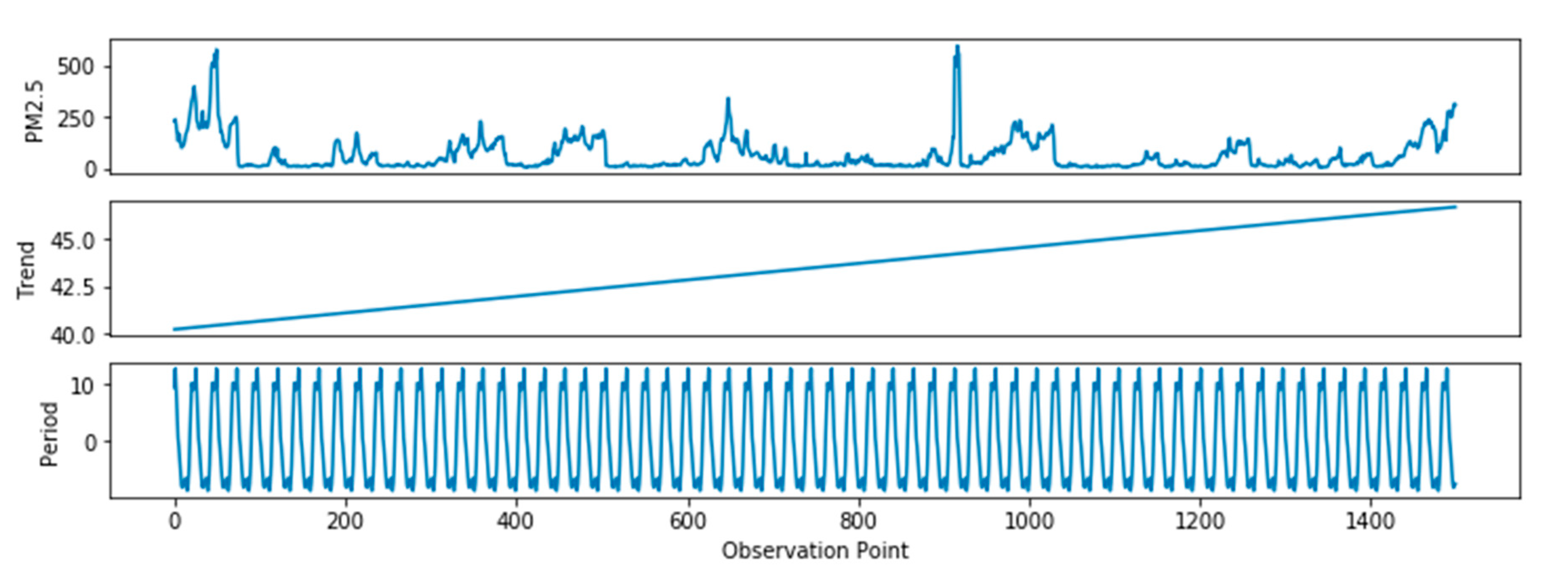
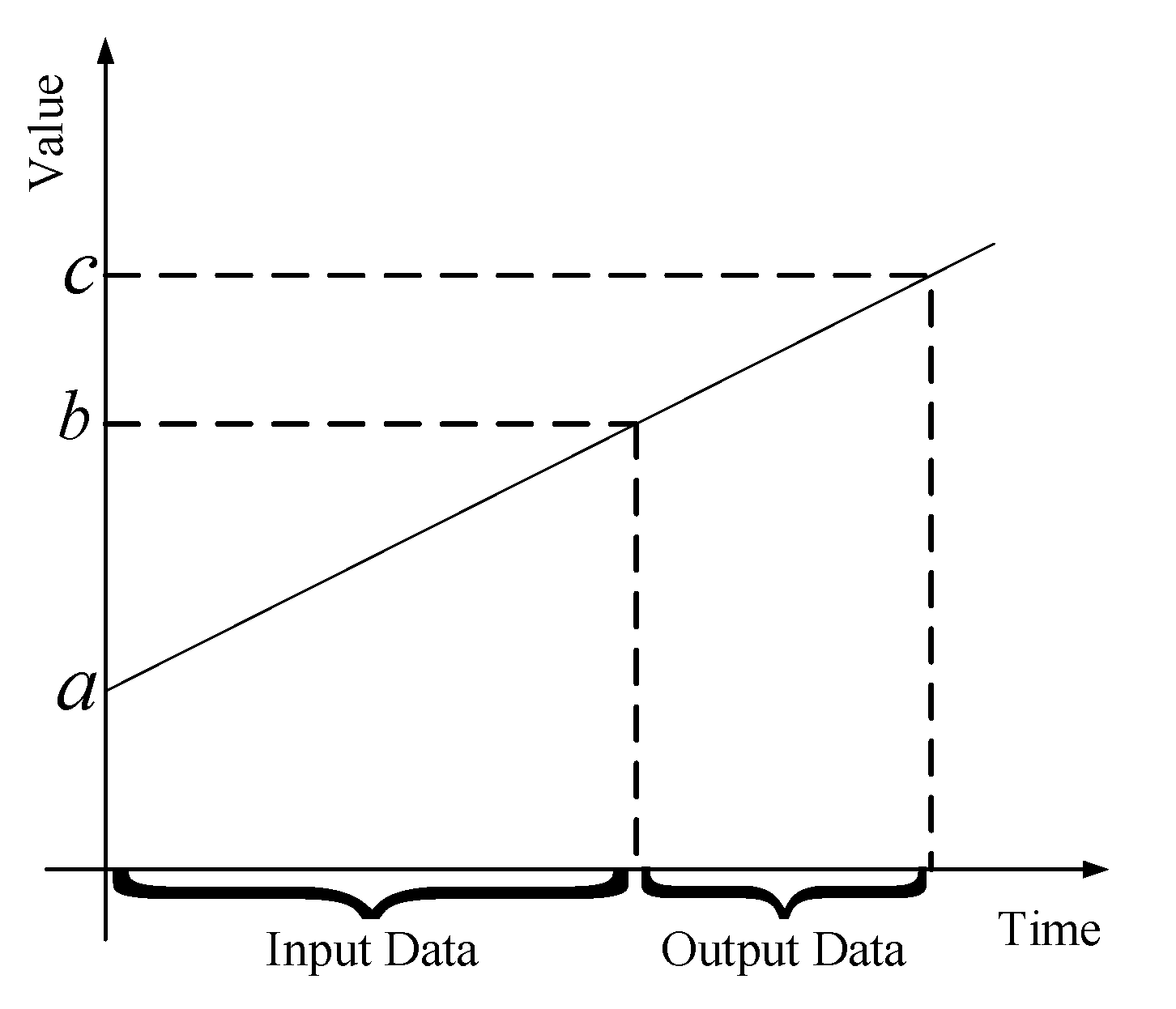
Trend component: This refers to the main trend direction of PM2.5 time-series data. This part often includes the trend of linear growth and decline. The trend component in PM2.5 data reflects the pollution of weather over a long period of time. If there are negative effects such as industrial pollution and automobile exhaust, the trend component of PM2.5 will exhibit linear growth. Conversely, if the air quality improves, the trend component of PM2.5 data will slowly decrease.

(2)

Period component: This refers to the data fluctuation that occurs repeatedly over a period of time. We found that the PM2.5 data had obvious period characteristics in one day; that is, the value during the day is higher and is lower than at night.

(3)

Residual component: This refers to the remaining part of the original data minus the trend and period components, and usually consists of complex nonlinear element and noise.

Figure 1 is an example of hourly PM2.5 average concentration data from January to February 2016 in Beijing, China, from which it can be seen that the trend in this period is upward from 40 μg/m³ to nearly 50 μg/m³. We know that Beijing is a northern city, and the winter season in Beijing from January to February is the heating season. Due to the burning of natural gas during the heating season, and the fact that winter 2016 was a warm winter without strong winds in Beijing, the air quality continued to worsen, so the PM2.5 value slowly increased.

Moreover, the periodicity within 24 h was very obvious between day and night. From the changes in each day, we can conclude that human and industrial activities during the day such as car trips and factory production will contribute to the PM2.5 increase. In contrast, at night, such activities are relatively reduced, so the PM2.5 concentration will decrease.

In this paper, we propose an integrated predictor of decomposing PM2.5 into three components such as the trend, period, and residual component, and give different predictors for each sub-sequence (i.e., the ARIMA model for the trend component and two GRU networks for period component and residual, respectively). The rest of the paper is organized as follows. Section 2 proposes the algorithmic framework for the time series prediction, especially the decomposition and the prediction model. To further explore and explain the applicability of the proposed model, experiments on the datasets of Beijing PM2.5 are illustrated in Section 3. Section 4 discusses the ability of deep learning networks to model linear time-series data, and analyzes the reasons that the prediction performance of deep learning networks will decrease for the trend component. Finally, Section 5 summarizes and concludes the paper.

2. Distributed Decomposition Model

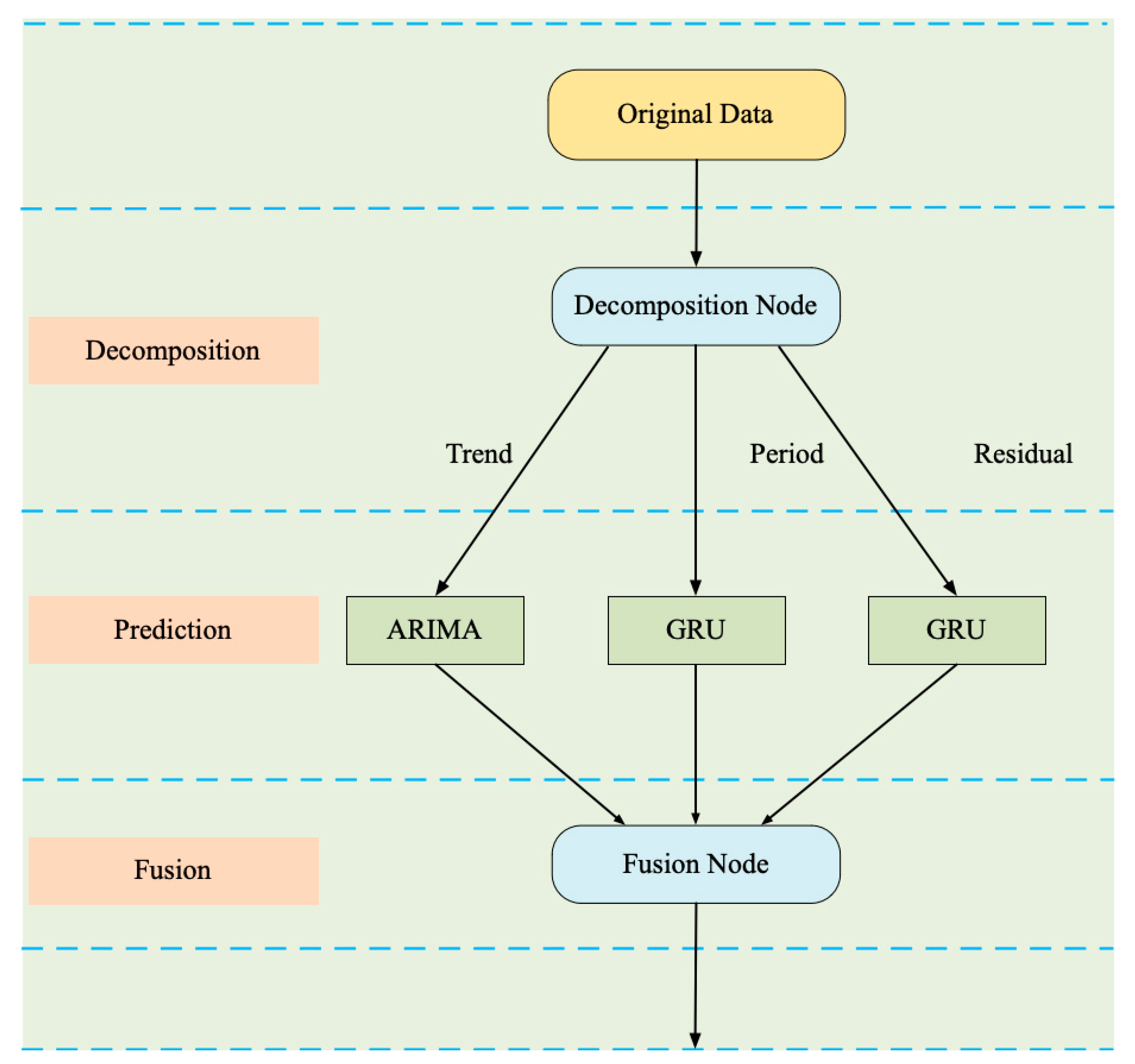
2.1. Model Framework

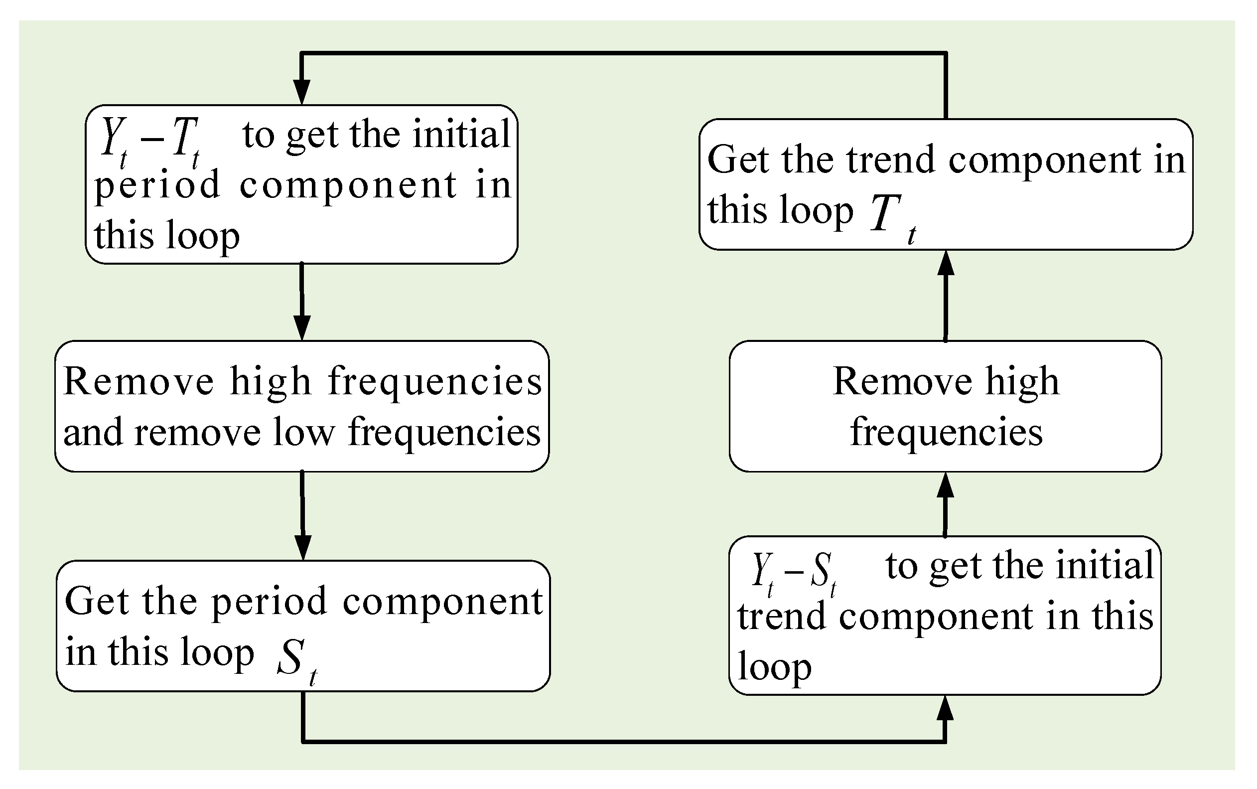
The model has three parts (i.e., decomposition, prediction, and fusion). In the decomposed node, the PM2.5 data are decomposed to three subsequences. In the network training stage, each component is trained separately to obtain different sub-predictors (i.e., the trend component is trained to obtain ARIMA model, and the period and residual components are trained to obtain two GRUs).

The prediction framework is shown in Figure 2. In the prediction stage, the ARIMA model is used to obtain the prediction of the trend component, and two different GRUs are used to predict the period and residual components, respectively, before finally, all the predictions are added together to obtain the final predicted result in fusion node.

2.2. Decomposition

Assume that PM2.5 time-series data $Y_t$ has N data, which means t = 1, 2, …, N. The relation with $Y_t$ and its three independent components (i.e., trend, period, and residual), as shown in Equation (1).

$$Y_t=T_t+S_t+R_{t}t=1,2,\dots ,N$$

(1)

where $T_t$, $S_t$, and $R_t$ are the trend component, period component, and residual component, respectively. Then, we have to obtain these three components $T_t$, $S_t$, and $R_t$ from the one time-series data $Y_t$, but this is mathematically an unsolvable equation.

Each component has different frequency bands, that is, the trend and period component are in the low and middle band, respectively. We used the cycle calculation process, shown in Figure 3, to calculate the trend and period components until these two components tended to be stable and no longer changed. In order to start the loop operation, we assumed $T_t$ = 0 in the first loop. The time series is fitted iteratively until the trend and period component stabilize, and at the end of the cycle calculation process, the trend component $T_t$ and period component $S_t$ are extracted from the data series, and the residual component is obtained by

$$R_t=Y_t-T_t-S_t,t=1,2,\dots ,N$$

(2)

Figure 3 shows that the decomposition has two important steps: one is “Remove high frequencies”, and the other is “Remove low frequencies”. Next, we will discuss the method of these two steps.

To remove the high frequencies, we used the locally weighted scatterplot smoothing (LOESS) smoother, which is based on fitting a weighted polynomial regression for a given time of observation, where weights decrease with distance from the nearest neighbor [30]. LOESS is a combination of the local fitting of polynomials and iteratively weighted least squares. At each point x in the dataset, a linear or quadratic polynomial is fit using the weighted least squares, giving more weight to points near point x that need to be smoothed and less weight to points further away.

Suppose x is the point to be smoothed, $i$ is the number of data points around x to be smoothed, and $x^{\left(i\right)}$ is the point around x within the width $i$. We chose a Gaussian function as the weighting factor ${\omega }^{\left(i\right)}$

$${\omega }^{(i)}=\exp (-\frac{{(x^{(i)}-x)}^2}{2{\tau }^2})$$

(3)

where $\tau$ is a constant to be set. It is always set according to the number of the data, and for PM2.5, which is a complex nonlinear data, we suggest that it is set to $\tau$ as within [3,19]. The value of the regression function for the point is then obtained by evaluating the local polynomial for that data point. By minimizing the value of the following

$$F={{\displaystyle {\sum }_i{\omega }^{\left(i\right)}(y^{(i)}-{\theta }^T{x}^{(i)})}}^2$$

(4)

to find the $\theta$ parameter, then the smoothed value $\widehat{y}$ of point $x$ can be obtained by

$$\widehat{y}={\theta }^{T}x$$

(5)

and the LOESS fit is complete after the regression function values have been computed for each of the data points.

On the other hand, we used a high-pass filter with cutoff frequency to remove low frequency bands. Obviously, it is critical to ensure that the loop converges to the trend component and the period component. We chose the so called seasonal-trend decomposition procedure based on LOESS (STL) [31] to achieve the loop convergence.

The STL method can adaptively adjust parameters according to each cycle calculation, so it can obtain good performance in ensuring convergence, and has many applications in data decomposition [32]. Here, we have omitted the details of the STL in order to focus our work (please refer [31] for the details of STL).

2.3. Autoregressive-Integrated Moving Average (ARIMA) Model: Prediction Model for Trend Component

In this paper, the ARIMA $(p,d,q)$ model was used and applied to model the trend component $T_t$, by which the future value of $T_t$ is to be predicted based on the linear modeling function of the past trend value. As a consequence, the time-series data that are fed to ARIMA should be linear and stationary. It returns the dependent variable only to its lag value and the present and lag values of the random error term [33]. In terms of modeling, it is mainly divided into four steps as follows:

Step 1: Import the raw data sequence to be predicted;

Step 2: Use the augmented Dickey-Fuller (ADF) unit root test to determine whether the sequence is stable or not. If it is not stable, use differential tools to make it smooth, and record the difference order as “$d$”; if the sequence is stable, then d is set as “1”.

Step 3: Obtain the value of $p$ and of the ARIMA $(p,d,q)$ model by the graphical properties of the autocorrelation function and the partial autocorrelation function after differencing was analyzed for preliminary determination. In order to select the best fitting model, the order of the model was determined according to the minimum Akaike information criterion (AIC), and the calculation formula of AIC is as follows [34]:

$$AIC=2m-2\log (L)$$

(6)

where $m$ is the number of parameters in the model, and is the sum of $p$ and $q$, and $L$ is the maximum value of likelihood function for the ARIMA $(p,d,q)$ model.

The AIC is a measure of the likelihood and the number of parameters. In theory, the order $(p,q)$ generally does not exceed one tenth of the data length. In this study, the order was set within (0, 10) first, and then the value of AIC was sequentially calculated by traversing to form an AIC matrix. The input to the model is the training dataset, that is, the first 75% of the trend component. Finally, find the order $(p,q)$ corresponding to the minimum AIC value from the AIC matrix.

Step 4: Build the ARIMA $(p,d,q)$ model with the parameter ${\varphi }_i$ and ${\theta }_i$ for a variable $X_t$ as

$$\Phi (B){(1-B)}^d\cdot X_t=\Theta (B)\cdot {\epsilon }_t$$

(7)

where $\Phi (B)=(1-{\displaystyle \sum _{i=1}^p{\varphi }_i{B}^i})$ and $\Theta (B)=(1-{\displaystyle \sum _{i=1}^q{\theta }_i{B}^i})$ are polynomials in the lag operator $B$; ${\epsilon }_t$ is white noise; $p$ is the number of autoregressive terms; $q$ is the number of moving average terms; and $d$ denote the differencing step. In this study, $X_t$ was set as the trend component $T_t$ from the STL decomposition described in Section 2.2.

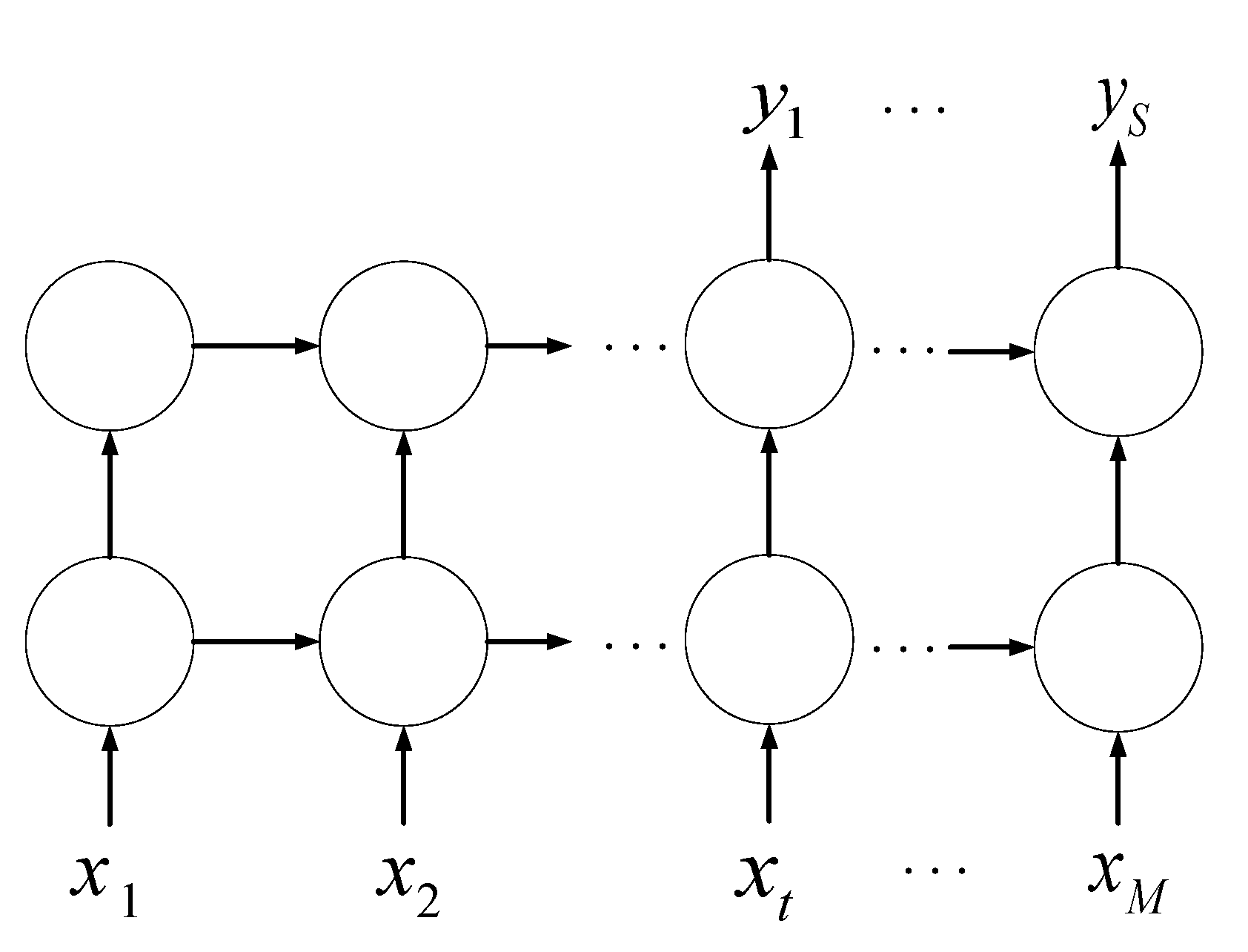
2.4. Gated Recurrent Unit (GRU) Network: Deep Prediction Network for Periodic and Residual Components

GRU is widely used for modeling because of its outstanding performance in sequence modeling. In order to solve the long-term dependency problem, the GRU architecture introduces a gating mechanism that can maintain the state of the cell for a long time. This method can solve the gradient problem of disappearing or exploding. The input data of GRU is the period component $S_t$ and residual component $R_t$.

The GRU contains these two gates:

• The update gate controls the degree to which the state information at a previous time is brought into the current state. The larger the value of the update gate, the more status information from a previous moment is brought in.
• The reset gate decides how much information is written to the current candidate activation ${\tilde{h}}_t$ in the previous state. The smaller the reset gate, the less information of the previous state is written.

Output from each GRU cell, ${\tilde{h}}_t$, is computed as [35]:

$$\begin{array}{l}{z}_t=\sigma (x_t{U}^z+h_{t-1}{W}^z+b^z)\\ r_t=\sigma (x_t{U}^r+h_{t-1}{W}^r+b^r)\\ {\tilde{h}}_t=\tanh (x_t{U}^h+(h_{t-1}\circ r_t)W^h+b^h)\\ h_t=(1-z_t)\circ {\tilde{h}}_t+z_t\circ h_{t-1}\end{array}$$

(8)

where $x_t$ is the input; $z_t$, $r_t$, ${\tilde{h}}_t$, and $h_t$ stand for the update gate, reset gate, current candidate activation, and activation of the GRU at time t, respectively; $U^z$, $U^r$, $U^h$, $W^z$, $W^r$, and $W^h$ are weight matrices to be learned during model training; $\circ$ is an element-wise multiplication; and $\sigma$ and tanh are commonly used nonlinear activation functions, whose mathematical form are as follows:

$$\sigma (x)=\frac{1}{1+e^{-x}}$$

(9)

$$\tanh (x)=\frac{e^x-e^{-x}}{e^x+e^{-x}}$$

(10)

Using the known input and output data, the network is trained by the stochastic gradient descent algorithm, and the optimal weight can be obtained. The GRU network is trained by the decomposed period and residual components. The GRU network consists of multiple GRU cells, and usually has several layers of structure. Shown as Figure 4, $x_t(t=1,2,\dots ,M)$ is the input of the GRU network, and $y_S(S=1,2,\dots ,N)$ is the output.

3. Experiments

3.1. Dataset and Experimental Setup

In this study, the PM2.5 measurement dataset was from the U.S. Department [36], which included 8784 records of hourly Beijing PM2.5 average concentration data from January to December 2016. We selected the first 75% of data for training and the remaining 25% as the test set.

The open source deep learning library Keras, based on Tensorflow, was used to build the learning models. All of the experiments were performed on a PC server with an Intel CORE CPU i5-4200U at 1.60 GHz, with 4 GB of memory. In the experiments, the default parameters in Keras were used for deep neural network initialization (e.g., weight initialization). GRU was designed with two layers, and the input and output dimensions were determined according to the number of input and output data. GRU models used the Adam optimized algorithm to obtain model parameters by optimizing a predetermined objective function. For the ARIMA model, we obtained the model parameters according to the rules described in Section 2.3, and we finally obtained the ARIMA model to predict the trend component.

Two cases were compared to show that the proposed model was effective for the prediction of PM2.5. From Case 1 (mentioned in Section 3.3), we can conclude that it is effective to decompose and predict with different sub-predictor, especially, when using ARIMA as the sub-predictor. From Case 2 (mentioned in Section 3.4), by comparing it with the results from [3], the results showed that the proposed model has the advantage in long-term prediction.

3.2. Evaluation of Prediction Results

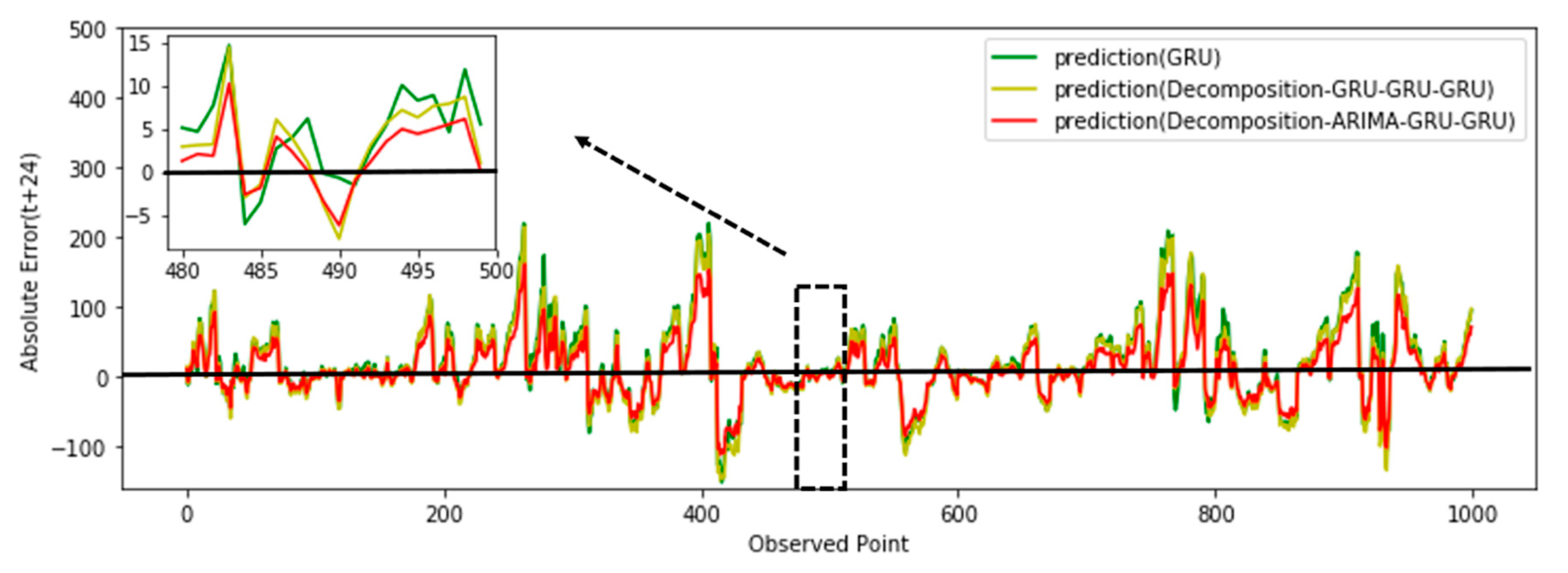
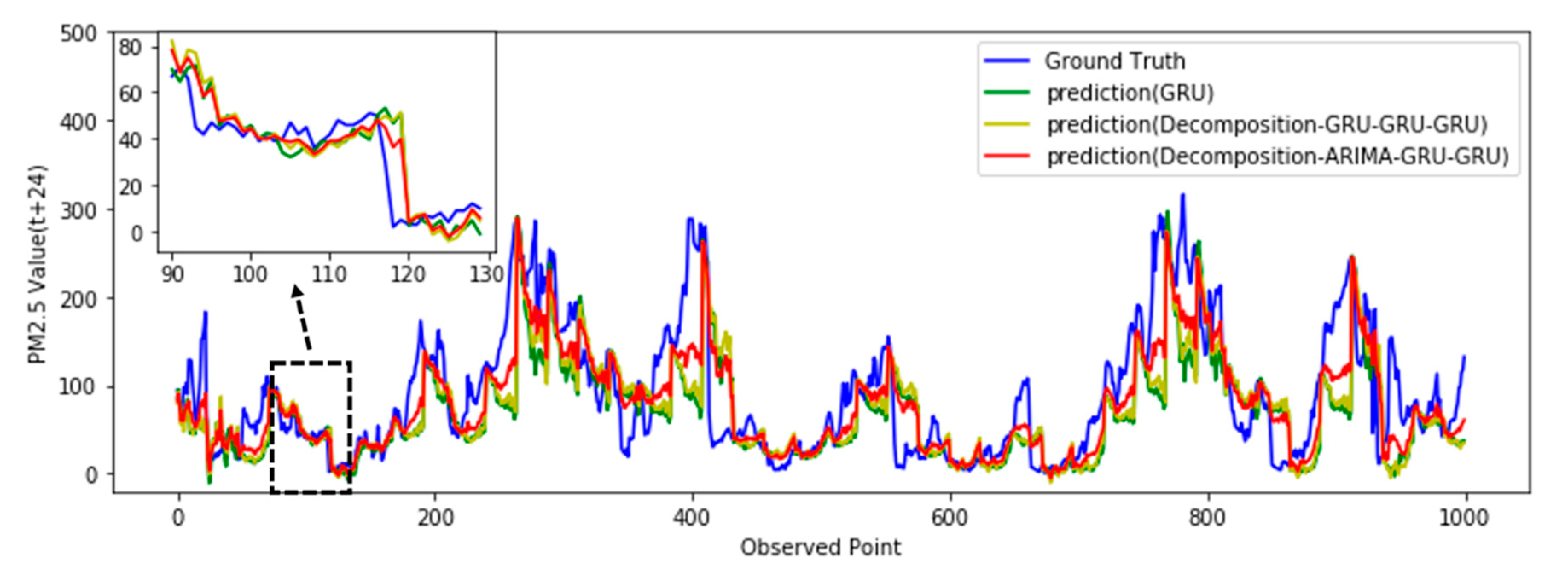
The prediction performance of different models was evaluated by comparing the prediction errors. Four quantitative evaluation indicators such as root mean square error (RMSE), normalized root mean square error (NRMSE), mean absolute error (MAE), and symmetric mean absolute percentage error (SMAPE) were used to evaluate the performance of the models. Furthermore, we utilized the Pearson correlation coefficient (R) to measure the linear relationship between the prediction and actual data. Their calculation formulas are shown in Equations (11)–(16).

In addition, we visualized the absolute error between the actual data and prediction values, as shown in Equation (16), which reflects the magnitude of the predicted value from the observed value.

$$RMSE=\sqrt{\frac{{{\displaystyle {\sum }_{i=1}^N(x_{pre}(i)-x_{obs}(i))}}^2}{N}}$$

(11)

$$NRMSE=\frac{1}{\max (x_{pre})-\min (x_{pre})}\sqrt{\frac{{{\displaystyle {\sum }_{i=1}^N(x_{pre}(i)-x_{obs}(i))}}^2}{N}}$$

(12)

$$MAE=\frac{1}{N}{\displaystyle {\sum }_{i=1}^N\left|x_{pre}(i)-x_{obs}(i)\right|}$$

(13)

$$SMAPE=\frac{1}{N}{\displaystyle {\sum }_{i=1}^N\frac{\left|x_{obs}(i)-x_{pre}(i)\right|}{(\left|x_{obs}(i)\right|+\left|x_{pre}(i)\right|)/2}}$$

(14)

$$R=\frac{{\displaystyle {\sum }_{i=1}^N(x_{obs}(i)-{\overline{x}}_{obs}(i))(x_{pre}(i)-{\overline{x}}_{pre}(i))}}{\sqrt{{\displaystyle {\sum }_{i=1}^N{(x_{obs}(i)-{\overline{x}}_{obs}(i))}^2{\displaystyle {\sum }_{i=1}^N{(x_{pre}(i)-{\overline{x}}_{pre}(i))}^2}}}}$$

(15)

$$AE=x_{pre}-x_{obs}$$

(16)

where $N$ is the number of predictive datasets; $x_{obs}$ represents the PM2.5 data, namely, ground truth value and $x_{pre}$ is predicted value; $\max (x_{pre})$ represents the maximum of predictive data; $\min (x_{pre})$ represents the minimum of predictive data; ${\overline{x}}_{obs}$ represents the average of PM2.5; and ${\overline{x}}_{pre}$ represents the average of prediction.

Obviously, RMSE, NRMSE, MAE, and SMAPE will be a non-negative number, and the smaller the values of these errors, the more accurate the predictions. The maximum value of R is 1, and a higher value of R indicates a better fit between the prediction and original data.

3.3. Case 1

Using the Beijing PM2.5 average concentration dataset mentioned in Section 3.1, we compared the proposed model with the following two models by predicting 24 h ahead for the PM2.5 average concentration:

• The GRU method [37]: The original time-series data are not decomposed, and the GRU is directly trained to establish a prediction model.
• Decomposition with the GRU-GRU-GRU method: The original time-series data are first decomposed according the method mentioned in Section 2.2, then the three components are trained to establish three sub-prediction GRU models. We can observe that this method is different from the model proposed here because it modeled the trend component by GRU, while in the proposed model, named in Figure 5 as decomposition, it was with ARIMA-GRU-GRU, which modeled the trend component by ARIMA.

The 24 steps in predicting the results of the PM2.5 concentration with three different models are shown in Figure 5. The blue line shows the ground truth (i.e., PM2.5 measurements), while the green, yellow, and red lines are the predicted results from GRU, decomposition-GRU-GRU-GRU, and decomposition with ARIMA-GRU-GRU, respectively. As can be seen from the figure, the prediction result of the proposed model was closer to the ground truth line. Figure 6 shows the absolute error (given by Equation (16)) between the predicted results and the PM2.5 time series. The green, yellow, and red lines are the absolute error curves of the GRU, decomposition-GRU-GRU-GRU, and the proposed model (decomposition with ARIMA-GRU-GRU), respectively. Figure 6 illustrates that the absolute error (AE) of the proposed model could obtain more values around 0, which indicates that a more accurate prediction had been achieved.

The comparisons of the RMSE, NRMSE, MAE, SMAPE, and R are shown in

Table 1. Comparison of the 24-step (24 h) prediction results.

Model	RMSE	NRMSE	MAE	SMAPE	R
GRU [37]	83.0925	0.1848	56.3784	0.7133	0.6389
Decomposition-GRU-GRU-GRU model	81.2412	0.1625	56.1870	0.7398	0.6471
The proposed Decomposition-ARIMA -GRU-GRU model	80.1620	0.1612	55.1060	0.6682	0.6508

. It can be seen that the proposed model obtained the least RMSE, NRMSE, MAE, and SMAPE, and the highest R, where the proposed model (RMSE 80.1620, NRMSE 0.1612, MAE 55.1060, SMAPE 0.6682, and R 0.6508) showed an improvement in prediction performance when compared to the GRU (RMSE 83.0925, NRMSE 0.1848, MAE 56.3784, SMAPE 0.7133, and R 0.6389) and decomposition-GRU-GRU-GRU (RMSE 81.2412, NRMSE 0.1625, MAE 56.1870, SMAPE 0.7398, and R 0.6417).

The RMSE, NRMSE, MAE, and SMAPE of the proposed model were 3.53%, 12.77%, 2.26%, and 6.32% lower than the GRU model, respectively, and the R value was increased by 1.86%. Compared with the decomposition-GRU-GRU-GRU model, the corresponding error indicators were reduced by 1.33%, 0.80%, 1.92%, and 9.68%, respectively, and the R value was increased by 0.57%. From the above data, the proposed model had better predictive performance. Although there was a slight outperformance, the training parameters of the ARIMA model were much fewer than the GRU model. Therefore, using the ARIMA model can simplify the model size and shorten the training time.

3.4. Case 2

In this case, by using the dataset mentioned in Section 3.1, we compared the proposed model to that in [3], that is, the experiment of predicting the forward 10 steps of the PM2.5 average concentration data.

Table 2. Comparison of 10-step (10 h) prediction results.

Model	RMSE	NRMSE	MAE	SMAPE	R
SLI-ESN [3]	65.7108	0.1966	46.0633	0.5443	0.7314
The proposed Decomposition-GRU-GRU-GRU model	59.4658	0.1237	37.5384	0.4520	0.8136

shows the statistical accuracy of the predictions by different models, as indicated by RMSE, NRMSE, MAE, SMAPE, and R.

Table 2 indicates that the proposed model (decomposition with ARIMA-GRU-GRU) outperformed the SLI-ESN model with a smaller predictive error for the 10-step prediction. The RMSE were 9.50%, 37.08%, 18.51%, and 16.96% lower than the SLI-ESN model, and the correlation coefficient R was above 0.8, and higher than SLI-ESN, which represents a stronger relationship between the prediction and the original PM2.5 data.

4. Discussion

We observed that the proposed model outperformed the GRU [37] and SLI-ESN [3]; moreover, it is important to use different sub-predictors to process different components of original data separately. In particular, the results showed that the ARIMA $(2,1,0)$ model could obtain a better performance in predicting the trend component than the neural network GRU. In this section, we will discuss the reason as the following.

The neural network needs to normalize the input data before, and then perform inverse normalization in the output step. The general methods to normalize are as follows:

$$x^{\prime }=\frac{x-x_{\min }}{x_{\max }-x_{\min }}$$

(17)

where $x^{\prime }$ is the normalized data; $x$ is original input data; $x_{\min }$ is the minimum of $x$; and $x_{\max }$ is the maximum of $x$. Then, the inverse normalization formula is

$$\widehat{x}=(x_{\max }-x_{\min })*\widehat{x}{}^{\prime }+x_{\min }$$

(18)

where $\widehat{x}{}^{\prime }$ is the prediction with the value within [0, 1] and $\widehat{x}$ is the inverse normalization value of $\widehat{x}{}^{\prime }$.

As shown in Figure 7, the minimum value of the input data is $a$, and the maximum value is $b$. In the normalization, this numerical range $[a,b]$ of the input data is mapped to $[0,1]$ by Equation (17). After the operation of the network, the predicted value is obtained, but within [0, 1], and then the inverse normalization calculation is required.

However, the network cannot predict the interval of the predicted value as [b, c], and the current inverse normalization method still uses the normalized interval to perform the operation, that is, $x_{\min }$ is $a$ and $x_{\max }$ is $b$. This is the basic reason for the inaccuracy of using neural networks to make regression predictions.

While the ARIMA model does not need the normalization and inverse normalization process, it can work well when data exhibit stable or consistent patterns over time. Moreover, the greater the slope of the trend component, the more obvious the advantages of using the ARIMA model. Therefore, we used the ARIMA model to model and predict the trend component, and obtained more accurate results than neural network GRU. The proposed methods proposed in this paper can combine other identification approaches [38,39,40,41,42] to study the modeling and prediction problems of other dynamic time series and stochastic systems with colored noises [43,44,45,46,47], and can be applied to other fields [48,49,50,51,52] such as signal modeling and control systems [53,54,55,56].

5. Conclusions

The PM2.5 time series has three components (i.e., trend, period, and residual components). The trend component changes slowly over time, which can be understood as slow changes in climate conditions. The period component shows the change in each day, with a slightly higher value during the day, and is lower at night. This is in line with the laws of actual climate change. Moreover, the decomposition could reduce the modeling difficulty of PM2.5 data and obtain more accurate prediction results, especially for the long-term prediction.

It is critical to choose the corresponding prediction models for different components. In this study, we used the ARIMA model to model and predict the trend component, and GRU networks were selected to model the period and residual components to capture the nonlinearity of the PM2.5 data.

The experimental results show that, first, decomposition is necessary to effectively reduce the difficulty of modeling the PM2.5 data. Second, using different models, especially using the ARIMA model, for the trend component is more accurate than the GRU; and finally the long-term prediction performance was improved simultaneously with fewer parameters and lower calculating cost.

References

1. Rybarczyk, Y.; Zalakeviciute, R. Machine learning approaches for outdoor air quality modelling: A systematic review. Appl. Sci. 2018, 8, 2570. [Google Scholar] [CrossRef]
2. Zhang, J.; Ding, W. Prediction of air pollutants concentration based on an extreme learning machine: The case of Hong Kong. Int. J. Environ. Res. Public Health 2017, 14, 114. [Google Scholar] [CrossRef] [PubMed]
3. Xu, X.; Ren, W. Prediction of Air Pollution Concentration Based on mRMR and Echo State Network. Appl. Sci. 2019, 9, 1811. [Google Scholar] [CrossRef]
4. Ding, F. Two-stage least squares based iterative estimation algorithm for CARARMA system modeling. Appl. Math. Model. 2013, 37, 4798–4808. [Google Scholar] [CrossRef]
5. Ding, F. Decomposition based fast least squares algorithm for output error systems. Signal Process. 2013, 93, 1235–1242. [Google Scholar] [CrossRef]
6. Pan, J.; Jiang, X.; Wan, X.K.; Ding, W. A filtering based multi-innovation extended stochastic gradient algorithm for multivariable control systems. Int. J. Control Autom. Syst. 2017, 15, 1189–1197. [Google Scholar] [CrossRef]
7. Ding, F.; Liu, X.P.; Liu, G. Gradient based and least-squares based iterative identification methods for OE and OEMA systems. Digit. Signal Process. 2010, 20, 664–677. [Google Scholar] [CrossRef]
8. Wang, Y.J.; Ding, F.; Wu, M.H. Recursive parameter estimation algorithm for multivariate output-error systems. J. Frankl. Inst. 2018, 355, 5163–5181. [Google Scholar] [CrossRef]
9. Liu, Q.Y.; Ding, F.; Xu, L.; Yang, E.F. Partially coupled gradient estimation algorithm for multivariable equation-error autoregressive moving average systems using the data filtering technique. IET Control Theory Appl. 2019, 13, 642–650. [Google Scholar] [CrossRef]
10. Ding, F.; Liu, X.G.; Chu, J. Gradient-based and least-squares-based iterative algorithms for Hammerstein systems using the hierarchical identification principle. IET Control Theory Appl. 2013, 7, 176–184. [Google Scholar] [CrossRef]
11. Wan, L.J.; Ding, F. Decomposition- and gradient-based iterative identification algorithms for multivariable systems using the multi-innovation theory. Circuits Syst. Signal Process. 2019, 38, 2971–2991. [Google Scholar] [CrossRef]
12. Zhang, X.; Ding, F.; Xu, L.; Yang, E.F. State filtering-based least squares parameter estimation for bilinear systems using the hierarchical identification principle. IET Control Theory Appl. 2018, 12, 1704–1713. [Google Scholar] [CrossRef]
13. Zhang, X.; Ding, F.; Xu, L.; Yang, E.F. Highly computationally efficient state filter based on the delta operator. Int. J. Adapt. Control Signal Process. 2019, 33, 875–889. [Google Scholar] [CrossRef]
14. Ni, X.Y.; Huang, H.; Du, W.P. Relevance analysis and short-term prediction of PM2.5 concentrations in Beijing based on multi-source data. Atmos. Environ. 2017, 150, 146–161. [Google Scholar] [CrossRef]
15. Wang, W.; Niu, Z. VAR Model of PM2.5, Weather and Traffic in Los Angeles-Long Beach Area. In Proceedings of the 2009 International Conference on Environmental Science and Information Application Technology, Wuhan, China, 4–5 July 2009. [Google Scholar]
16. Wang, B.; Zhao, Z.; Nguyen, D.D.; Wei, G.W. Feature functional theory–binding predictor (FFT–BP) for the blind prediction of binding free energies. Theor. Chem. Acc. 2017, 136, 55. [Google Scholar] [CrossRef]
17. Zhu, H.; Lu, X. The prediction of PM2.5 value based on ARMA and improved BP neural network model. In Proceedings of the 2016 International Conference on Intelligent Networking and Collaborative Systems, Ostrawva, Czech Republic, 7–9 September 2016. [Google Scholar]
18. Chen, Y. Prediction algorithm of PM2.5 mass concentration based on adaptive BP neural network. Computing 2018, 100, 825–838. [Google Scholar] [CrossRef]
19. Liu, C.; Shu, T.; Chen, S.; Wang, S.; Lai, K.K.; Lu, G. An improved grey neural network model for predicting transportation disruptions. Expert Syst. Appl. 2016, 45, 331–340. [Google Scholar] [CrossRef]
20. Haiming, Z.; Xiaoxiao, S. Study on prediction of atmospheric PM2.5 based on RBF neural network. In Proceedings of the 2013 Fourth International Conference on Digital Manufacturing & Automation, Qingdao, China, 29–30 June 2013. [Google Scholar]
21. García-Mozo, H.; Oteros, J.A.; Galán, C. Impact of land cover changes and climate on the main airborne pollen types in Southern Spain. Sci. Total Environ. 2016, 548, 221–228. [Google Scholar] [CrossRef]
22. Jesús, R.; Rivero, R.; Jorge, R.-M.; Federico, F.-G.; Rosa, P.-B. Modeling pollen time series using seasonal-trend decomposition procedure based on LOESS smoothing. Int. J. Biometeorol. 2017, 61, 335–348. [Google Scholar]
23. Ming, F.; Yang, Y.X.; Zeng, A.M.; Jing, Y.F. Analysis of seasonal signals and long-term trends in the height time series of IGS sites in China. Sci. China Earth Sci. 2016, 59, 1283–1291. [Google Scholar] [CrossRef]
24. Rumelhart, D.E. Learning representations by back-propagating errors. Nature 1986, 23, 533–536. [Google Scholar] [CrossRef]
25. Hochreiter, S.; Schmidhuber, J. Long short-term memory. Neural Comput. 1997, 9, 1735–1780. [Google Scholar] [CrossRef] [PubMed]
26. Cho, K.; Van Merrienboer, B.; Gulcehre, C.; Bahdanau, D.; Bougares, F.; Schwenk, H.; Bengio, Y. Learning phrase representations using RNN encoder-decoder for statistical machine translation. In Proceedings of the Conference on Empirical Methods in Natural Language Processing, Doha, Qatar, 25–29 October 2014. [Google Scholar]
27. Zhao, X.; Zhang, R.; Wu, J.L.; Chang, P.C. A deep recurrent neural network for air quality classification. J. Inf. Hiding Multimed. Signal Process 2018, 9, 346–354. [Google Scholar]
28. Huang, C.J.; Kuo, P.H. A deep cnn-lstm model for particulate matter (PM2.5) forecasting in smart cities. Sensors 2018, 18, 2220. [Google Scholar] [CrossRef]
29. Pak, U.; Ma, J.; Ryu, U.; Ryom, K.; Juhyok, U.; Pak, K.; Pak, C. Deep learning-based PM2.5 prediction considering the spatiotemporal correlations: A case study of Beijing, China. Sci. Total Environ. 2019. [Google Scholar] [CrossRef]
30. Dagum, E.B.; Luati, A. Global and local statistical properties of fixed-length nonparametric smoothers. Stat. Methods Appl. 2002, 11, 313–333. [Google Scholar] [CrossRef]
31. Cleveland, R.B.; Cleveland, W.S.; McRae, J.E.; Terpenning, I. STL: A seasonal-trend decomposition procedure based on loess. J. Off. Stat. 1990, 6, 3–73. [Google Scholar]
32. Zhou, J.; Liang, Z.; Liu, Y.; Guo, H.; He, D.; Zhao, L. Six-decade temporal change and seasonal decomposition of climate variables in Lake Dianchi watershed (China): Stable trend or abrupt shift. Theor. Appl. Climatol. 2015, 119, 181–191. [Google Scholar] [CrossRef]
33. Box, G.; Gwilym, M.; Gregory, C.; Greta, M. Time Series Analysis: Forecasting and Control, 1st ed.; John Wiley & Sons: Hoboken, NJ, USA, 2015; pp. 93–123. [Google Scholar]
34. Libert, G. A New Look at the Statistical Model Identification. Automat. Control IEEE Trans. 1974, 19, 716–723. [Google Scholar]
35. Huang, Q.; Wang, W.; Zhou, K.; You, S.; Neumann, U. Scene labeling using gated recurrent units with explicit long range conditioning. arXiv 2016, arXiv:1611.07485. [Google Scholar]
36. Mission China. Available online: http://www.stateair.net/web/historical/1/1.html (accessed on 20 July 2017).
37. Xie, R.; Ding, Y.; Hao, K.; Lei, C.; Tong, W. Using gated recurrence units neural network for prediction of melt spinning properties. In Proceedings of the 2017 11th Asian Control Conference (ASCC), Gold Coast, Australia, 17–20 December 2017. [Google Scholar]
38. Zhang, X.; Ding, F.; Yang, E.F. State estimation for bilinear systems through minimizing the covariance matrix of the state estimation errors. Int. J. Adapt. Control Signal Process. 2019, 33, 1157–1173. [Google Scholar] [CrossRef]
39. Ma, H.; Pan, J.; Ding, F.; Xu, L.; Ding, W. Partially-coupled least squares based iterative parameter estimation for multi-variable output-error-like autoregressive moving average systems. IET Control Theory Appl. 2019, 13. [Google Scholar] [CrossRef]
40. Li, M.H.; Liu, X.M.; Ding, F. The filtering-based maximum likelihood iterative estimation algorithms for a special class of nonlinear systems with autoregressive moving average noise using the hierarchical identification principle. Int. J. Adapt. Control Signal Process. 2019, 33, 1189–1211. [Google Scholar] [CrossRef]
41. Liu, S.Y.; Ding, F.; Xu, L.; Hayat, T. Hierarchical principle-based iterative parameter estimation algorithm for dual-frequency signals. Circuits Syst. Signal Process. 2019, 38, 3251–3268. [Google Scholar] [CrossRef]
42. Liu, L.J.; Ding, F.; Xu, L.; Pan, J.; Alsaedi, A.; Hayat, T. Maximum likelihood recursive identification for the multivariate equation-error autoregressive moving average systems using the data filtering. IEEE Access 2019, 7, 41154–41163. [Google Scholar] [CrossRef]
43. Ma, J.X.; Xiong, W.L.; Chen, J.; Ding, F. Hierarchical identification for multivariate Hammerstein systems by using the modified Kalman filter. IET Control Theory Appl. 2017, 11, 857–869. [Google Scholar] [CrossRef]
44. Ma, J.X.; Ding, F. Filtering-based multistage recursive identification algorithm for an input nonlinear output-error autoregressive system by using the key term separation technique. Circuits Syst. Signal Process. 2017, 36, 577–599. [Google Scholar] [CrossRef]
45. Ma, P.; Ding, F. New gradient based identification methods for multivariate pseudo-linear systems using the multi-innovation and the data filtering. J. Frankl. Inst. 2017, 354, 1568–1583. [Google Scholar] [CrossRef]
46. Ding, F.; Wang, F.F.; Xu, L.; Wu, M.H. Decomposition based least squares iterative identification algorithm for multivariate pseudo-linear ARMA systems using the data filtering. J. Frankl. Inst. 2017, 354, 1321–1339. [Google Scholar] [CrossRef]
47. Gu, Y.; Ding, F.; Li, J.H. States based iterative parameter estimation for a state space model with multi-state delays using decomposition. Signal Process. 2015, 106, 294–300. [Google Scholar] [CrossRef]
48. Gu, Y.; Ding, F.; Li, J.H. State filtering and parameter estimation for linear systems with d-step state-delay. IET Signal Process. 2014, 8, 639–646. [Google Scholar] [CrossRef]
49. Ding, F. Combined state and least squares parameter estimation algorithms for dynamic systems. Appl. Math. Model. 2014, 38, 403–412. [Google Scholar] [CrossRef]
50. Ding, F. Coupled-least-squares identification for multivariable systems. IET Control Theory Appl. 2013, 7, 68–79. [Google Scholar] [CrossRef]
51. Ding, F. Hierarchical multi-innovation stochastic gradient algorithm for Hammerstein nonlinear system modeling. Appl. Math. Model. 2013, 37, 1694–1704. [Google Scholar] [CrossRef]
52. Liu, Y.J.; Ding, F.; Shi, Y. An efficient hierarchical identification method for general dual-rate sampled-data systems. Automatica 2014, 50, 962–970. [Google Scholar] [CrossRef]
53. Ding, F.; Liu, G.; Liu, X.P. Partially coupled stochastic gradient identification methods for non-uniformly sampled systems. IEEE Trans. Autom. Control 2010, 55, 1976–1981. [Google Scholar] [CrossRef]
54. Ding, J.; Ding, F.; Liu, X.P.; Liu, G. Hierarchical least squares identification for linear SISO systems with dual-rate sampled-data. IEEE Trans. Autom. Control 2011, 56, 2677–2683. [Google Scholar] [CrossRef]
55. Wang, Y.J.; Ding, F. Novel data filtering based parameter identification for multiple-input multiple-output systems using the auxiliary model. Automatica 2016, 71, 308–313. [Google Scholar] [CrossRef]
56. Ding, F.; Liu, Y.J.; Bao, B. Gradient based and least squares based iterative estimation algorithms for multi-input multi-output systems. Proc. Inst. Mech. Eng. Part I J. Syst. Control Eng. 2012, 226, 43–55. [Google Scholar] [CrossRef]
Figure 1. Decomposition of PM2.5 time series in Beijing, China.
Applsci 09 04533 g001
Figure 2. Flowchart of the prediction framework.
Applsci 09 04533 g002
Figure 3. Flowchart of decomposition.
Applsci 09 04533 g003
Figure 4. Network structure of the gated recurrent unit (GRU) network.
Applsci 09 04533 g004
Figure 5. Comparison between the predicted results and ground truth (24 steps).
Applsci 09 04533 g005
Figure 6. Absolute error between the predicted results and ground truth (24 steps).
Applsci 09 04533 g006
Figure 7. Normalization and inverse normalization of linear prediction using neural networks.
Applsci 09 04533 g007