Article

Bayesian Proxy Modelling for Estimating Black Carbon Concentrations using White-Box and Black-Box Models

1
Institute for Atmospheric and Earth System Research/Physics, Helsinki University, FI-00560 Helsinki, Finland
2
School of Public Health and Social Work, Queensland University of Technology, Queensland 4000, Australia
3
Lyles School of Civil Engineering, Purdue University, West Lafayette, IN 47907, USA
4
Ray W. Herrick Laboratories, Center for High Performance Buildings, Purdue University, West Lafayette, IN 47907, USA
5
Department of Physics, The University of Jordan, Amman 11942, Jordan
*
Authors to whom correspondence should be addressed.
Appl. Sci. 2019, 9(22), 4976; https://doi.org/10.3390/app9224976
Submission received: 15 October 2019 / Revised: 14 November 2019 / Accepted: 15 November 2019 / Published: 19 November 2019
(This article belongs to the Special Issue Air Quality Prediction Based on Machine Learning Algorithms)

Abstract

:
Black carbon (BC) is an important component of particulate matter (PM) in urban environments. BC is typically emitted from gas and diesel engines, coal-fired power plants, and other sources that burn fossil fuel. In contrast to PM, BC measurements are not always available on a large scale due to the operational cost and complexity of the instrumentation. Therefore, it is advantageous to develop a mathematical model for estimating the quantity of BC in the air, termed a BC proxy, to enable widening of spatial air pollution mapping. This article presents the development of BC proxies based on a Bayesian framework using measurements of PM concentrations and size distributions from 10 to 10,000 nm from a recent mobile air pollution study across several areas of Jordan. Bayesian methods using informative priors can naturally prevent over-fitting in the modelling process and the methods generate a confidence interval around the prediction, thus the estimated BC concentration can be directly quantified and assessed. In particular, two types of models are developed based on their transparency and interpretability, referred to as white-box and black-box models. The proposed methods are tested on extensive data sets obtained from the measurement campaign in Jordan. In this study, black-box models perform slightly better due to their model complexity. Nevertheless, the results demonstrate that the performance of both models does not differ significantly. In practice, white-box models are relatively more convenient to be deployed, the methods are well understood by scientists, and the models can be used to better understand key relationships.

Graphical Abstract

1. Introduction

1.1. Motivation

Seven million people die each year due to the adverse health effects of air pollution, with 4.2 million deaths attributed to exposure to ambient (outdoor) air pollution [1]. Approximately 91 % of the world’s population lives in areas where air pollution exceeds guideline limits established by the World Health Organization (WHO) [2]. Several health-relevant ambient air pollutants include carbon monoxide (CO), ozone (O 3 ), nitrogen oxides (NO and NO 2 ), sulfur dioxide (SO 2 ), and particulate matter (PM) [3]. Atmospheric PM has become the subject of extensive research due to its impact on human health, ecosystems, and the climate [4]. A critically important class of atmospheric PM is ultrafine particles (UFPs), which are particles smaller than 100 nm in size. UFPs have very high surface area to mass ratios and preferentially deposit in the tracheobronchial and alveolar regions of the human respiratory system. A large fraction of UFPs are derived from emissions associated with traffic, industrial activities, and domestic heating [5]. UFPs tend to dominate atmospheric PM number size distributions and contribute little to PM mass concentrations that are presently used as air quality indicators (e.g., PM 2.5 and PM 10 ). Thus, particle number (PN) concentrations are more useful in describing the abundance of UFPs [6].
In addition to UFPs, another health-relevant component of atmospheric PM is black carbon (BC). BC is emitted from the incomplete combustion of carbonaceous material and is associated with vehicle exhaust, coal-fired power plants, and biomass burning for heating and cooking [7]. BC is an important component of PM in cities, contributing 5 % 15 % to the total PM mass concentrations in urban air [8,9]. BC has negative implications for human health [10], regional and global climate [11], and extreme weather events [12]. Due to its relatively short lifetime in the atmosphere [13], it has been suggested that mitigation of BC emissions may reduce global warming [10].
Due to the aforementioned BC impacts, the United Nations Environmental Programme recommends monitoring this pollutant in cities side-by-side with other air pollution indicators (such as PM 2.5 and CO) for the purpose of mitigation and adaptation policy making and planning. In practice, BC measurement is not as trivial as other pollutant indicators [14,15] and it is expensive (a proper BC measurement setup is on the order of approximately $50,000) to plan in some situations. Complications with data acquisition, such as instrument failure, data corruption, and calibration frequency, can lead to missing BC data during research campaigns or continuous measurements [16]. Standard interpolation methods are ineffective to fill such data gaps if they are relatively long in duration. BC levels have been shown to vary proportionally with those of traffic-related gaseous pollutants, such as CO, NO, and NO 2 [6]. Therefore, it may be possible to estimate BC mass concentrations using other air pollution metrics and indicators. Such an approach can help fill critical gaps in the measurement of BC that has long been hindered by instrumentation cost and measurement complexity. In order to address the aforementioned challenges, we propose the development of BC proxies through a data-driven model with a Bayesian framework. A BC proxy can be defined as a mathematical model that estimates BC mass concentrations using other available measured variables, such as levels of PM or gaseous pollutants. Deriving a proxy for BC is in many cases cost efficient and accurate. BC, PM 2.5 , CO, and NO x originate from similar urban air pollution sources; thus, presently existing monitoring stations and their databases can be used to estimate BC concentrations not only in the present/future, but also historically. In this study, we introduce BC proxies that are based upon PM measurements by establishing relationships between BC and size-fractionated PM concentrations.

1.2. Data-Driven Air Pollution Models

Air pollution models are typically developed through three approaches: physics- and expert-based methods and data-driven methods. Physics-based approaches directly model the underlying physical processes related to air quality variables [17]. Examples include the Urban Airshed Model (UAM) [18] and the Community Multiscale Air Quality (CMAQ) model [19]. Expert-based approaches, such as the expert elicitation process [20], elicit knowledge from specialists for modelling and analysis [21]. Data-driven methods establish models by identifying relationships and trends in historical data sets. Combinations of these models, for example, including expert information into data-driven methods, can also be used.
Physics-based approaches are typically sensitive to several factors, including computational resources, the scale and quality of the parameters involved, and dependency on large databases of several input parameters, some of which may not always be available [22,23]. Likewise, the use of expert systems is not always straightforward and it is often difficult to find agreement among experts on how the uncertainties of different variables can be adequately accounted for [20]. Recently, more practitioners have resorted to data-driven approaches, such as neural networks, as alternatives to physics- and expert-based methods [24]. Typically, data-driven methods do not require an in-depth understanding of air pollutant dynamics and other explanatory variables. However, the use of expert or known information may guide the inclusion of key variables and provide information about the nature of the expected relationship (e.g., linear or non-linear). Such methods can take advantage of the growth in low-cost air pollution sensing networks and computing technologies [25].
In particular, BC analysis has been investigated extensively such as described in [26,27]. BC modelling is also well developed, which mostly consists of physics-based models. Examples include the global transport model [28], regional climate-atmospheric chemistry model [29], land use regression models [30], and the BC mixing state model [31]. Recently, BC has been modelled using statistical distributions [32] and the linear mixed-effect model [33]. However, these models do not act as a proxy where BC concentrations can be estimated using other measured variables.
While data-driven methods have been extensively used as other air pollutant estimators, a major issue is the lack of proper interpretation of the results due to the usage of non-transparent models (e.g., black-box (BB) models). Uncertainty analysis is also often neglected when the model outcomes are point-based estimates [24]. To overcome such issues, we develop a white-box (WB) model to predict BC mass concentrations using PM and PN data. The developed model for the BC proxy is then integrated with a Bayesian framework to address over-fitting and uncertainty quantification issues that typically arise in a modelling process. A Bayesian BB model is also developed for comparison.

2. Case Study: Jordan Air Pollution Measurement Campaign

The proposed BC proxy methodology will be tested on air quality data sets obtained from a mobile measurement campaign performed at several locations in Jordan, including the two most populated urban areas in the country: Amman and Zarqa. This campaign took place from 29 May to 4 June 2014. The sampling interval was 30 s for the aethalometer and 10 s for the remaining instruments used in this campaign. The data was then further pre-processed for analysis and proxy development by taking the average to be one minute per data point. The campaign map and other detailed information about measurement campaign are described by Hussein et al. [34].
The measurements represent one of the most comprehensive mobile campaigns involving PM number concentrations and size distributions down to the UFP regime in urban areas in the Middle East and North Africa (MENA) region [35]. Understanding air pollutant sources in the area is a challenge: Amman is known as the economic and political center of the country, whereas Zarqa is one of the industrial centers. Furthermore, air pollution in the southern part of Jordan is mainly affected by dust particles due to sand resuspension from desert areas [35]. Urban air pollution in Amman and Zarqa originates from a vast range of sources, including emissions from traffic and industrial activities, local-scale household activities involving the burning of biomass (e.g., heating in the winter), and natural sources (e.g., dust resuspension). Airborne dust (super-micron PM >1 μ m) is a major problem, not only in Jordan, but throughout the MENA region [36]. According to the majority of anthropogenic air pollutant sources in the area, BC is likely to be an important pollutant that contributes meaningfully to total PM concentrations.
The mobile campaign included the measurement of size-fractionated PM concentrations (10 nm–10 μ m) and BC mass concentrations. Table 1 lists the associated aerosol instrumentation and measured variables. Using several portable instruments that cover a wide size range and with different cutoff diameters makes it possible to derive particle number and mass concentrations in several size fractions. In this study, we focus on the following size fractions: submicron (0.01 μ m–1 μ m) particle number concentrations with three fractions in the following particle diameter ranges: 10 nm–20 nm, 20 nm–300 nm and 0.3 μ m–1 μ m. The PM x was obtained from the DustTrak, which recorded PM 1 , PM 2.5 , and PM 10 .
BC concentrations were measured with a portable aethalometer (microAeth, AethLabs model AE51), which reports the BC concentration based on changes in light attenuation at a wavelength of 880 nm of particles collected on a disposable filter. The filter was replaced each day prior to the measurements. The sample flow rate was 0.1 L/min and a 2.5 μ m size selective inlet was used. We set the time-resolution at 30 s. The BC data was post processed to remove any spurious spikes in the concentration (e.g., >1000 μ g/m 3 ) that were associated with sudden vibration of the instrument. This type of monitor (i.e., microAeth AE51) was tested against a reliable type (aethalometer AE31) and also for real-time performance in field measurements. According to Cheng and Lin [37], negative BC levels may be present using AE51 at low actual BC levels or at a high time-resolution. Negative values can be eliminated very effectively by adopting the optimized noise-reduction averaging (ONA) algorithm.

3. Methods: Bayesian Modelling

Although physics-based models are often considered as WB models [38], statistical models that can explain how they behave, how they produce predictions, and what the influencing variables are, can also be categorized as WB models. This type of modelling is also known as WB machine learning [39,40]. Examples include linear and logistic regression, decision trees, and generalized additive models [41]. This section describes the details of the Bayesian methods for estimating BC concentrations in the forms of WB and BB models.

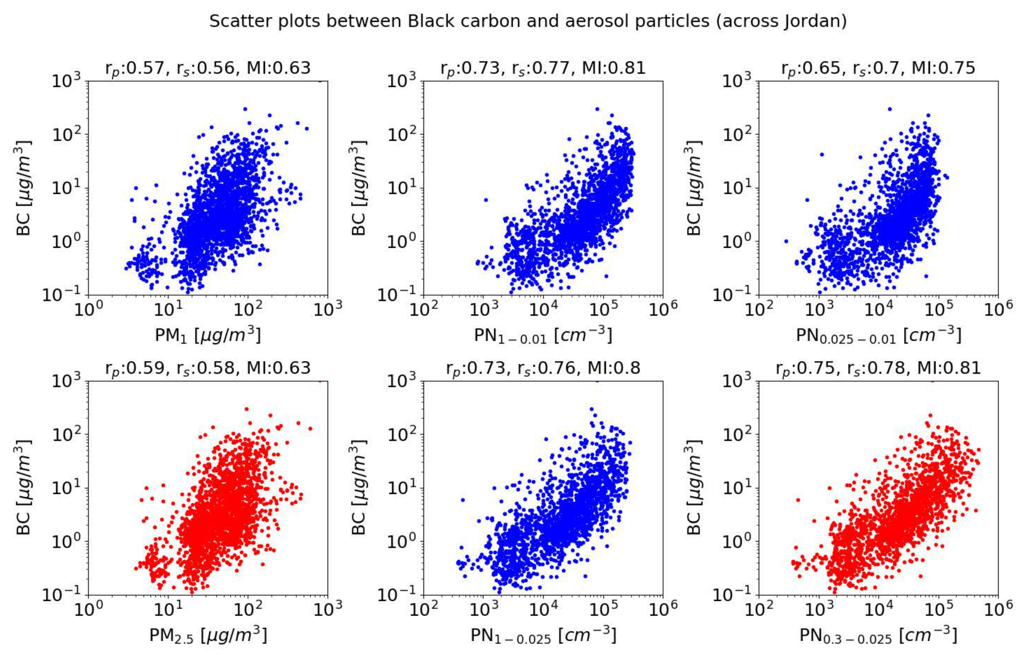
3.1. Features Analysis

The collection of aerosol instrumentation presented in Table 1 permits determination of size-fractionated PM mass concentrations, including PM 1 , PM 2.5 , and PM number concentrations (PN): 0.01–1 μ m (PN 1 0.01 ), 0.01–0.025 μ m (PN 0.025 0.01 ), 0.025–1 μ m (PN 1 0.025 ), and 0.025–0.3 μ m (PN 0.3 0.025 ).
The relationship between BC mass concentrations and size-fractionated PM mass and number concentrations is displayed in Figure 1. The use of all PM size fractions in the BC proxy may be redundant since some variables may have similar contributions and others may not have meaningful associations with BC. Therefore, it is important to analyse the features of the PM and PN concentrations. Three types of correlation analyses are performed including Pearson (r p ), Spearman (r s ), and mutual information (MI). The Pearson correlation coefficient is known to be effective for evaluating the linear relationship between two continuous variables [42], whereas the Spearman correlation coefficient is computed based on the ranked values for each variable rather than the raw data [43]. MI is also applied to ensure undetected non-linear correlations between these variables are captured [44,45].
The relationship between these variables and BC mass concentrations are shown on each subplot of Figure 1. From the correlation analysis, it can be seen that the correlations between each PM variable with BC mass concentrations does not differ significantly. In this case, the variables of PM 2.5 and PN 0.3 0.025 (shown as red data points in Figure 1) are selected as the features for the inputs of the BC proxy based on physical characteristics of BC. The size distribution of BC is known to be in the range of 25–300 nm and that fraction contributes significantly to PM 2.5 [9]. The use of the PM 2.5 variable is advantageous because it is typically included in routine air quality monitoring around the world [46] and is increasingly used as part of low-cost air quality sensing networks [47].

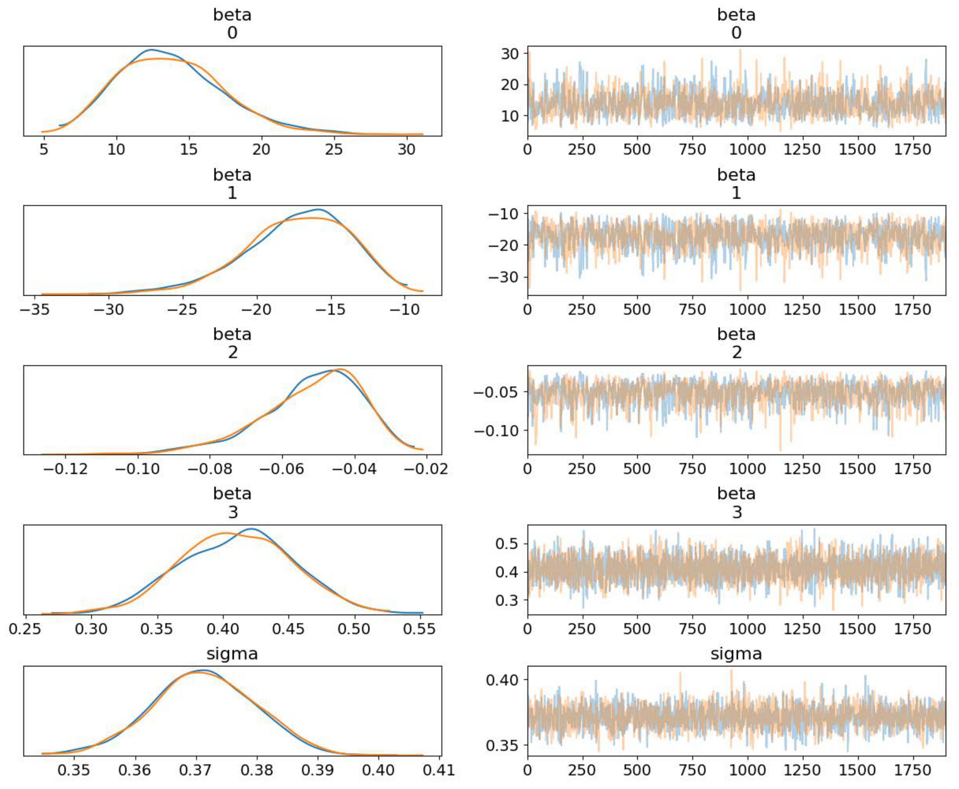
3.2. Bayesian Model: White Box

From the previous subsection, it is known that BC contributes to both PM 2.5 and PN 0.3 0.025 . From Figure 1, it is also known that the relationship between BC mass concentration with PM 2.5 and PN 0.3 0.025 on a logarithmic scale are linear and non-linear, respectively. Therefore, the proposed structure of BC proxy can then be written as:
log 10 [ BC ] = β 1 + β 2 log 10 [ PM 2.5 ] + β 3 e β 4 log 10 [ PN 0.3 0.025 ] + ε
The mathematical description of the proposed proxy structure can be simplified to be:
y = β 1 + β 2 X 1 + β 3 e β 4 X 2 + ε
where y , X 1 , and X 2 are log 10 [ BC ] , log 10 [ PM 2.5 ] , and log 10 [ PN 0.3 0.025 ] , respectively. The notation ε is a random error term that follows a Gaussian distribution, ε N ( 0 , σ 2 ) and σ 2 is a noise variance. Finally, the model coefficient is symbolized by β = { β 1 , β 2 , β 3 , β 4 } . The proxy based on Equation (2) can be considered as a WB model since the relationship between the inputs and output are visible and transparent.
The aim in Bayesian modelling is not only to find single “best” values of model coefficients ( β ), but rather to explicitly account for the uncertainty of the coefficient estimate using the posterior distributions of model coefficients. Bayes’ rule [48] can be defined as:
posterior likelihood × prior
The following sub-subsections will discuss the setup of the prior distribution and likelihood function and then describe the Bayesian inference for obtaining the posterior and predictive distributions.

3.2.1. Prior Distribution

The proxy coefficients are modelled as a Gaussian distribution, given by p ( β ) N ( μ 0 , σ 0 ) , whereas the noise variance is assumed as a random variable following an inverse Gamma distribution, given by p ( σ 2 ) IG ( a , b ) .
Informative priors are established by applying nonlinear regression on the training data. First, the variable, μ 0 , can be initiated using the estimated variables, ^ } β , where the standard deviation, σ 0 , is chosen to be twice that of the mean value, μ 0 . Second, the parameters a and b are estimated by taking the squared residual values between the nonlinear regression estimation and the real BC mass concentration data. This provides the residual mean, μ r , and its corresponding variance, σ r 2 . Using the properties of the inverse Gamma distribution, the parameter a can be estimated using a = ( μ r / σ r ) 2 + 2 , whereas the parameter b can be computed using b = μ r ( μ r / σ r ) 2 + 1 as proposed in Zaidan et al. [49], Zaidan et al. [50]. These prior parameters are then used as starting values for the chosen initiation method for running Markov Chain Monte Carlo (MCMC) algorithm.

3.2.2. Likelihood Function

The likelihood for this model is the conditional probability of observing the data ( X 1 and X 2 ) and the model parameters ( β , σ 2 ). The likelihood also follows a Gaussian distribution and it can be written as:
p ( y | X 1 , X 2 , β , σ 2 ) N ( y | β 1 + β 2 X 1 + β 3 e β 4 X 2 , σ 2 I )

3.2.3. Posterior and Predictive Distributions

Using the likelihood function and the prior distribution, the posterior distribution can be computed using Bayes’ theorem, shown in Equation (3), to give:
p ( β , σ 2 | y , X 1 , X 2 ) posterior dist . p ( y | X 1 , X 2 , β , σ 2 ) likelihood func . p ( β ) p ( σ 2 ) prior dist .
Since the probabilistic model above becomes non-linear, the exact inference is intractable. Hence, in order to estimate posterior distributions, we resort to the use of a sampling method, referred to as No-U-Turn Sampler (NUTS). NUTS is an MCMC algorithm that closely resembles Hamiltonian Monte Carlo [51]. To initialize the NUTS sampler, Automatic Differentiation Variational Inference (ADVI) [52] is used first, where instead of sampling the posterior, the parameters of a tractable distribution are fitted to match the posterior [53,54].
Once posterior distributions have been estimated using the NUTS algorithm, the predictive distribution can be computed by generating data from the model using the posterior draws from parameters. The implementation is done using PyMC3 [55].

3.3. Bayesian Model: Black Box

Neural networks can be considered as BB models since they provide little explanatory insight into the relative influence of the independent variables in the prediction process [56]. From a statistical perspective, neural networks are a robust approximator to estimate real-valued (prediction) and discrete-valued (classification) target functions because they can mimic the non-linearity of the functions and their learning methods are well-developed [57]. Neural networks and their family have been used in a large number of applications [58], including air pollution research [24]. In order to enable for a fair comparison with the Bayesian WB approach, here a Bayesian method is implemented into neural networks, known as a Bayesian neural network (BNN) [45].
A neural network, f ( X , β ) , can be viewed as a probabilistic model, that follows a Gaussian distribution, given by:
p ( y | X , β , γ ) N ( y | f ( X , β ) , γ 1 )
where the notations of X , β , and γ are the inputs, the neural network parameters (i.e., weights), and the precision of the Gaussian distribution, respectively. Equation (6) is also known as a likelihood function.
In a Bayesian framework, a prior distribution needs to be assigned, where in this case, the prior follows a Gaussian distribution with mean zero and the precision of α , given by:
p ( β | α ) N ( β | 0 , α 1 I )
Using the prior distribution and likelihood function, the posterior distribution for the BNN can be computed based on Bayes theorem, shown in Equation (3), to give:
p ( β | y , X , α , γ ) posterior dist . p ( y | X , β , γ ) likelihood func . p ( β | α ) prior dist .
The inclusion of the prior distribution leads to a regularization, which then counters over-fitting [59,60]. Furthermore, BNN provides a degree of belief on the estimated output, which can be used to assess the quality of the predictions. However, due to the non-linear dependence of f ( X , β ) on β , the posterior distribution calculation is intractable.
The first solution to estimate the BNN posteriors was proposed using a Laplace approximation [61,62]. Solutions to compute more accurate posterior distributions have been developed, including variational inference [63], sampling-based variational inference [64], and expectation propagation [65]. In this case, we adopt the recent solution based on automatic differentiation to variational inference (ADVI) proposed by Kucukelbir et al. [52], Blundell et al. [66]. This approach optimises the weights by minimising a compression cost, known as the variational free energy or the expected lower bound on the marginal likelihood.
The structural details of the BNN can be found in Hagan et al. [59], whereas the posterior based Bayesian optimisation can be found in Blundell et al. [66]. As with the Bayesian implementation of WB modelling, the BNN implementation also uses pyMC3 [55].

4. Results

This section discusses the BC proxy modelling process and explains the performance of the BC proxies.

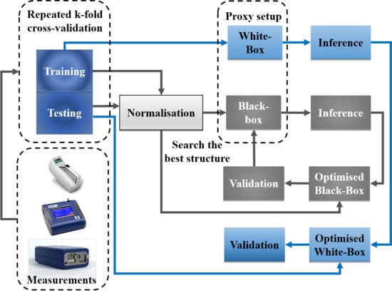
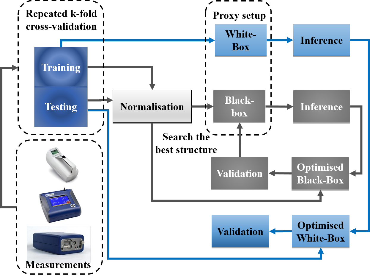
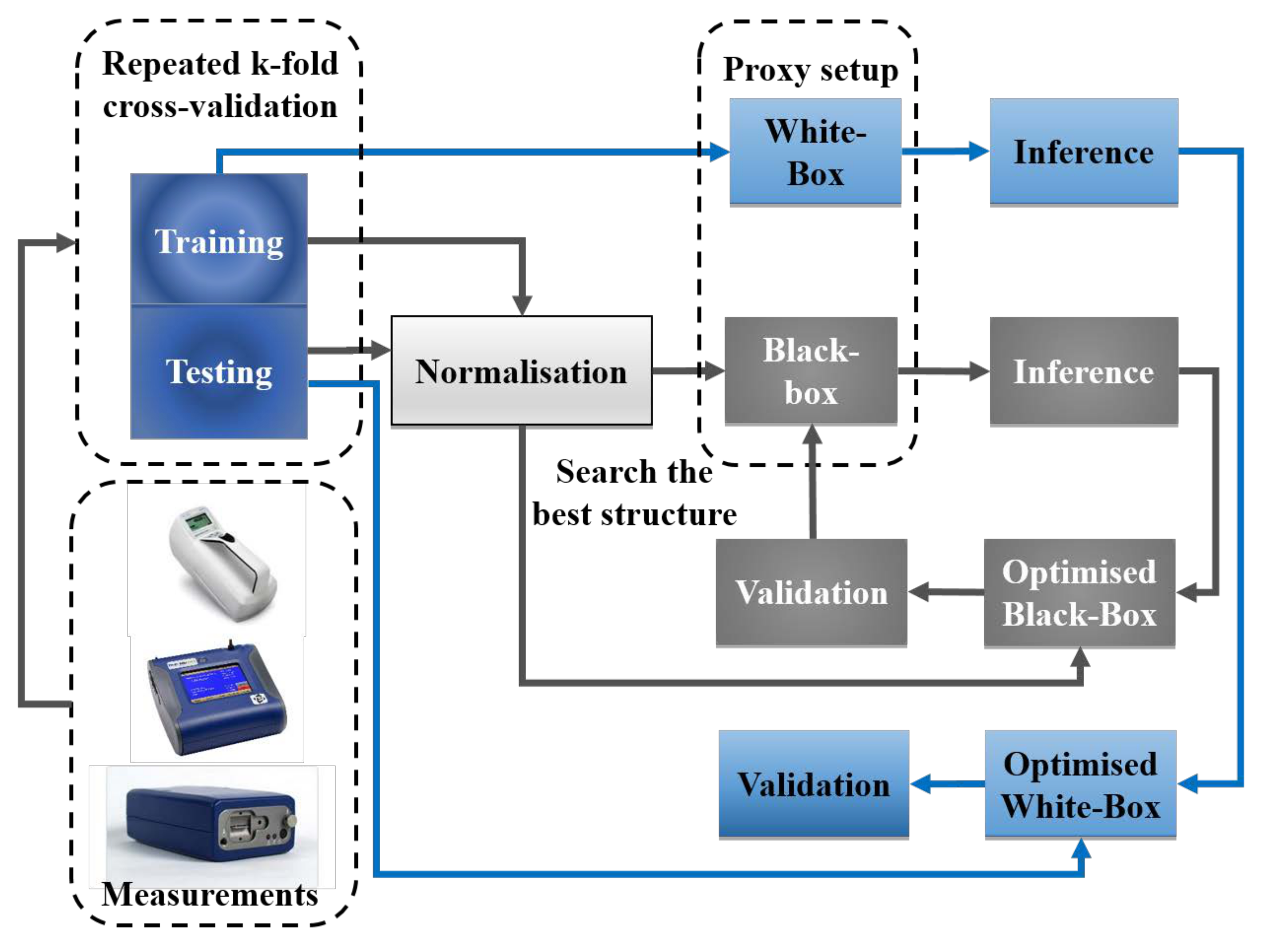
4.1. Modelling Process

As discussed in Section 3.1, the PM 2.5 and PN 0.3 0.025 data sets are used as inputs to the BC proxy, whereas BC data is assigned as the proxy’s output. K-fold cross-validation is used to select the training and testing data. The cross-validation is repeated many times with different randomization in each repetition, where the method is known as repeated k-fold cross-validation [67].
For the WB model, the proposed proxy structure, shown in Equation (1), is first established. Then the model coefficients of β and noise variance ( σ 2 ) can be estimated using the NUTS inference, as explained in Section 3.2. Multi-process sampling is performed on two core processors simultaneously (i.e., 2 chains in 2 jobs). Figure 2 shows an example of the posterior distribution of our parameters and the individual samples drawn. These include all model parameters that are β and σ . The colors blue and orange show two different samplings performed in parallel. It can be seen that the sampling chains for the individual parameters, shown in the subplots on the right hand side, converge well and are stationary (e.g., no large drifts or other odd patterns). As mentioned previously, the predictive distributions can then be obtained by generating data from the models using the estimated posterior distributions.
For the BB model, the data needs to first be normalized. In this way, the weight-input product is guaranteed to be small when initialising the network weights to small random values. The magnitudes of the weights also have a consistent meaning [59]. The next step is to setup the many possibilities of the BNN structures, including the different number of hidden layers, different activation functions on hidden layers, such as rectified linear unit (ReLU), sigmoid and hyperbolic tangent function (tanh) [68], and the number of neurons on each layer. We start the training from the simplest BNN structure first, then the results are validated using the testing data and the performance is recorded. The training and validation processes are performed iteratively by increasing the complexity of the BNN structure to find the best BNN structure.
For the BB model, it is not possible to run an MCMC sampler, such as NUTS, because the sampling will become very slow as the model is scaled up to deeper architectures with more layers and/or the number of neurons increases. Instead, the ADVI variational inference algorithm is used as mentioned in Section 3.3. The ADVI is based on a mean-field approximation such that the correlations in the posterior are neglected, with the advantage of being computationally much faster and scaling well to higher dimensions. The “brute-force” method is applied to find the best BNN structure using performance metrics, which are also used for model evaluation, as described in Section 4.2. It is then found that the most optimal BNN structure is one single hidden layer network with a ReLU function with 100 neurons.
Figure 3 shows the procedure of the WB and BB model developments. The database is established using the measurement campaign data as explained in Section 2. The data is then divided into training and testing data using repeated k-fold cross-validation. The parameter k is chosen between 2 and 10 and each process is repeated 50 times with different randomisation. The key differences between WB and BB development are in the normalisation method for the data sets applied to the BB model and the search of optimal structure for the BB model. The approaches utilised are computationally demanding, therefore these modelling process are performed in a super-cluster, provided by CSC-IT Center for Science Ltd. [69].

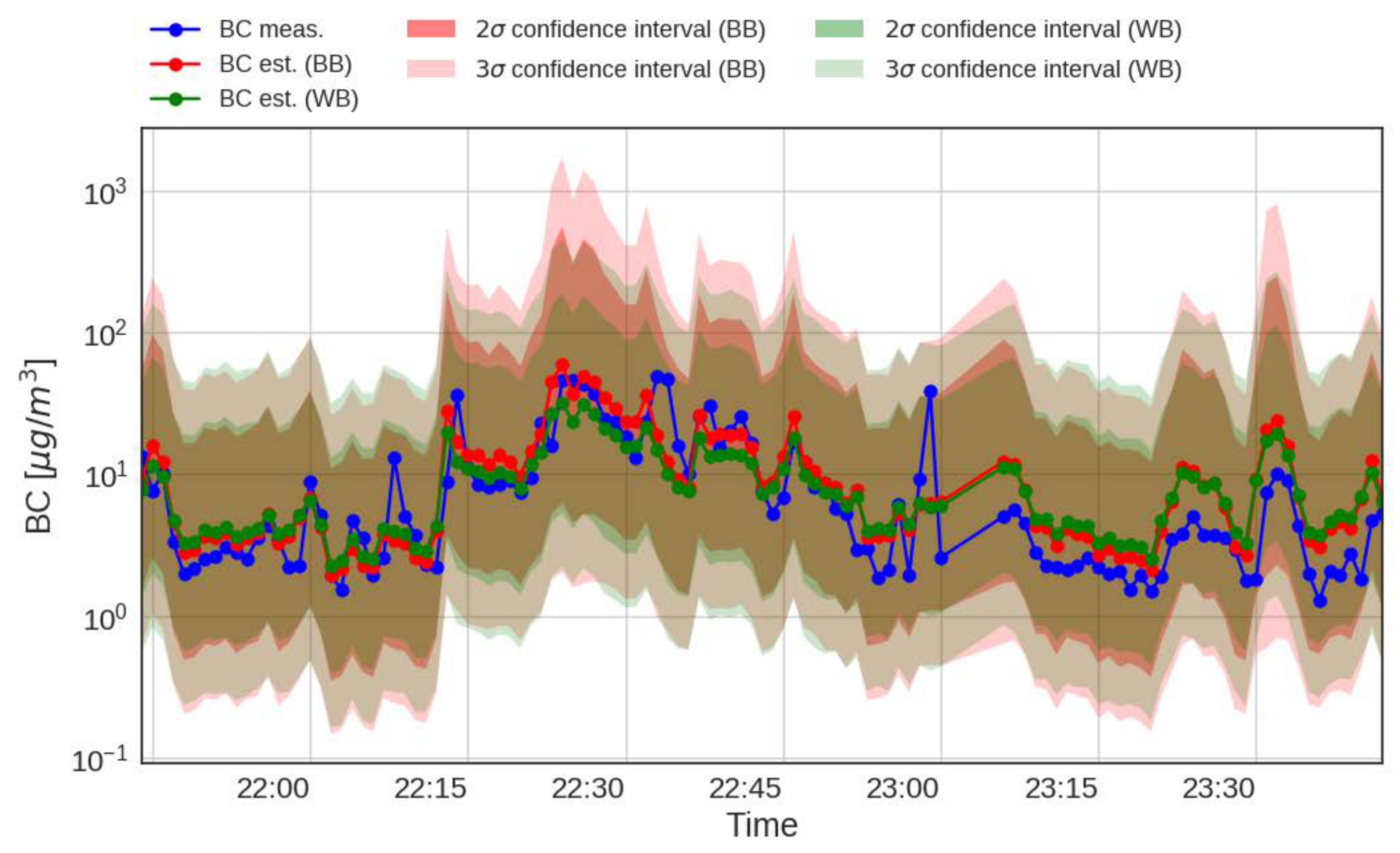
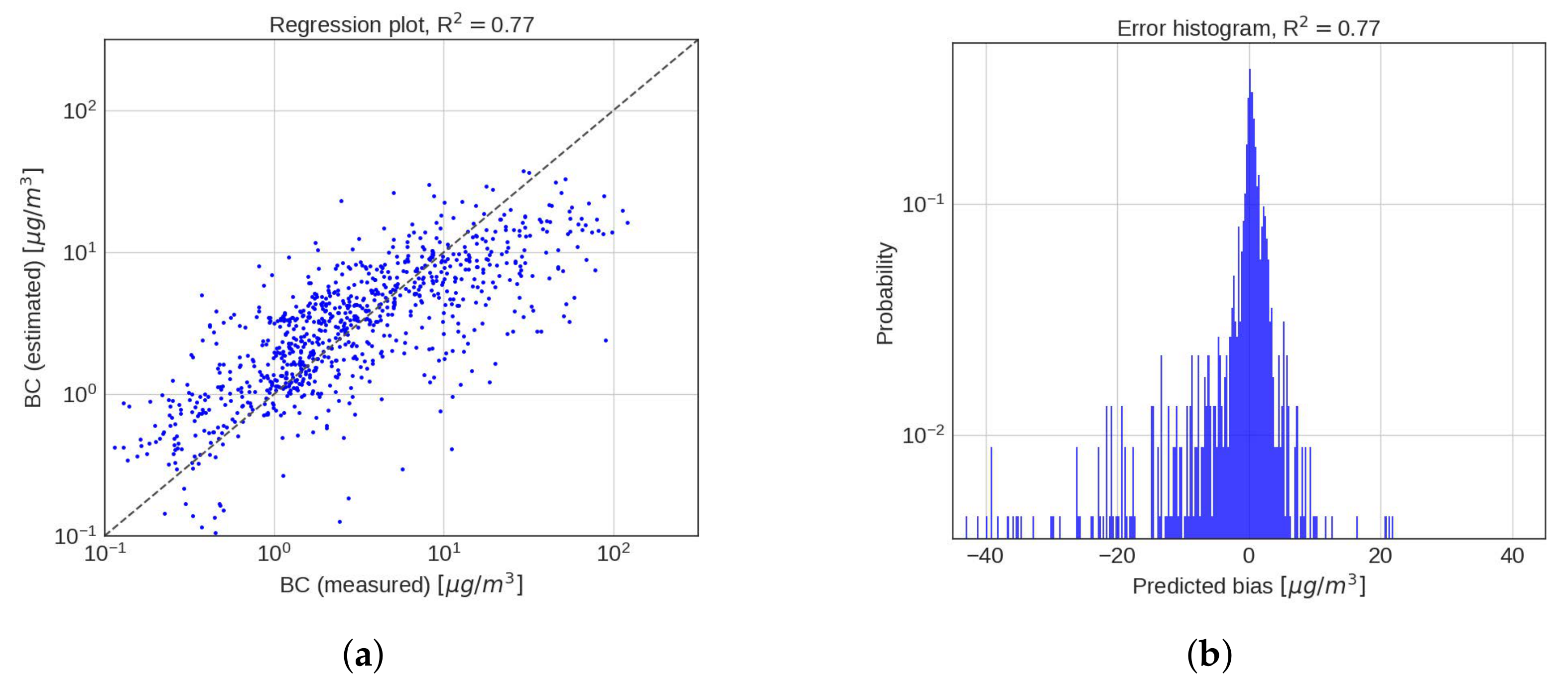
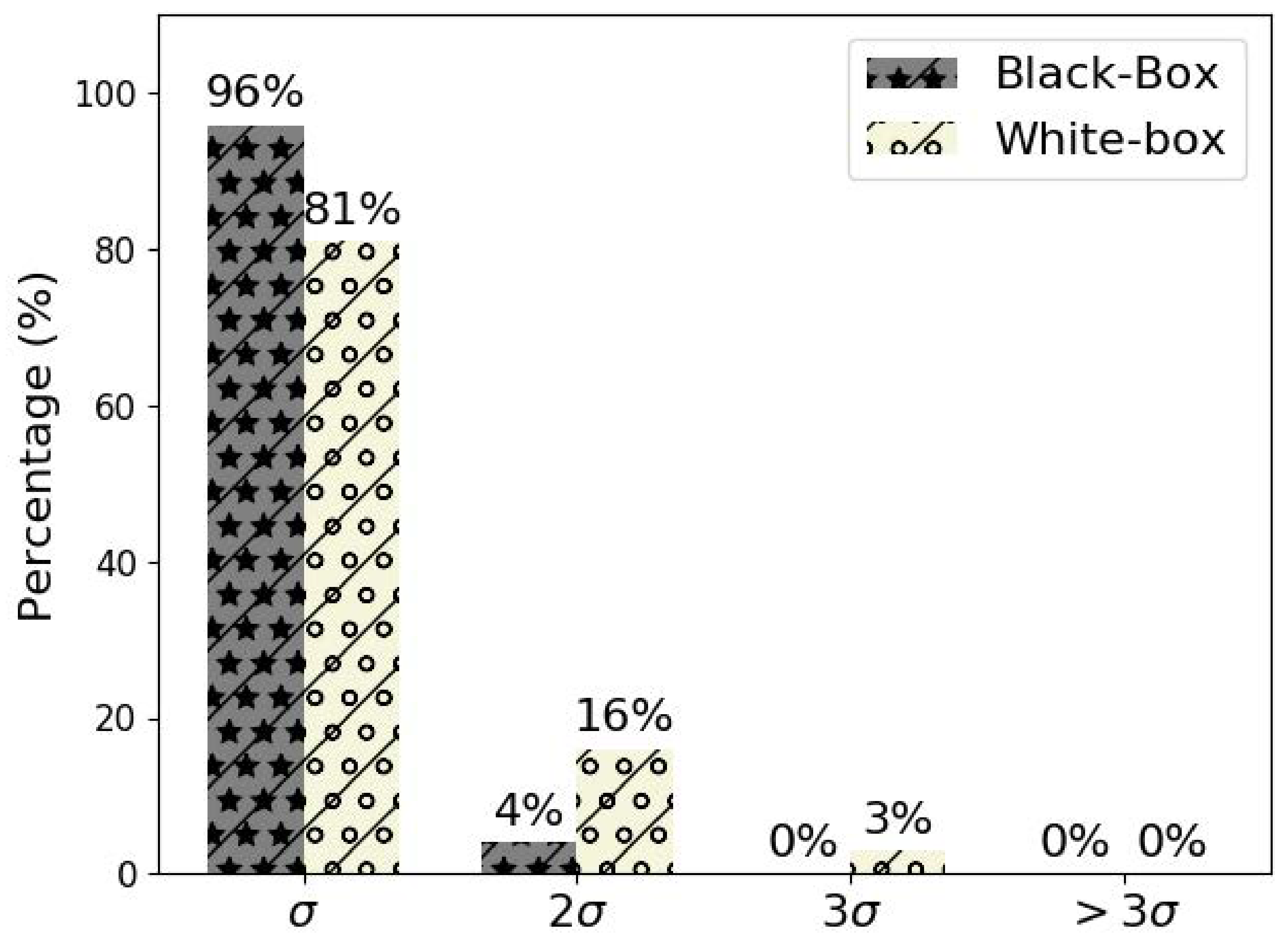
4.2. Performance Analysis

This subsection discusses the performance analysis of the developed BC proxies. Figure 4 shows a fraction of the time-series results of the BC proxies tested on data measured in Amman city center on 29 May 2014 from 21:44 to 23:42. The blue, red, and green lines represent the real BC measurement and the estimated BC quantity via the BB and WB proxies, respectively. The red and green light areas are 2 σ and 3 σ predicted uncertainty of their respected estimations. Even though the BC proxies do not fit perfectly the data points of BC measurement, it can be seen that both BC estimations track well the pattern of the BC measurement. Furthermore, the uncertainty estimations of 2 σ nearly cover the entire region of the BC measurement. Nevertheless, the time-series result only displays a snapshot in a particular area at particular time, it does not represent the overall performance metric of the proxy development results.
Three additional metrics are used to describe the overall quality of the BC proxy performance. The first metric is called the mean absolute error (MAE). It has a simple interpretation as the average absolute difference between the predicted proxy values ( y ^ ) and the real measurement data points ( y ). The second metric is the root mean squared error (RMSE), which is also known as the standard deviation of the residuals (prediction errors). The third metric is called the coefficient of determination, denoted by R 2 . It provides a measure of how well the observed outcomes are replicated by the proxy, based on the proportion of total variation of outcomes explained by the proxy. The summary of these three performance metrics is shown in the Table 2.
The proposed BC proxies are implemented on the data obtained from the measurements performed across urban areas (i.e., Amman and Zarqa) and throughout Jordan (including urban areas). The repeated k-fold cross-validation is used to establish training and test data sets. Using the performance metrics shown in Table 2, the performance of the proxies are then evaluated and the results are presented in Table 3. The low values of MAE and RMSE indicate that the proxy performance is better than the high values of these metrics. On the other hand, the high R 2 values indicate the proxy performance is better than the lower values. It can be seen here that in both cases and across different areas in Jordan, all performance metrics indicate that the BB model outperforms the WB model. However, it can be observed that the difference in the performance metric values are relatively small indicating that the performance of the WB and BB models are similar. In this case, considering the complexity of setting up the BB model, as well as its non-transparency, it is worthwhile to utilise the developed WB model for estimating BC measurements.
The following performance metrics will focus on the WB model development applied on the Jordan data. In addition to these three metrics, we present the WB model results as a regression plot and an error histogram (Figure 5). The regression plot displays the relationship between the outputs of the proxy (y-axis) and the real measurement data (x-axis) (Figure 5a). The error histogram shows the histogram of the difference between estimated proxy values and real measurement values (Figure 5b). From both figures, it can be observed that the results are adequate: most of estimated BC values lie close to the ground truth line in the regression plot (with R 2 is at 0.77 ), whereas the error histogram demonstrates that the highest probability (i.e., histogram peak) lies at zero. The latter means that the difference between the BC estimations and the BC measurements are mostly close to zero. These figures conclude that the developed WB proxy is adequate for field deployment under measurement conditions similar to those in urban areas of Jordan.

4.3. Discussion

This subsection discusses the advantages of using the developed proxy in terms of uncertainty analysis, as well as its potential to be embedded in low-cost PM sensors, and bias-variance trade-off in modelling choice.
Since we can directly estimate the uncertainty associated with our prediction using the (Bayesian) predictive distributions, we are able to quantify how many estimated BC data points fall within each degree of model uncertainty (standard deviation, symbolized as σ ). Figure 6 shows the bar chart of the percentage of estimated BC data points that lie within σ to 3 σ . It can be seen that about 81% and 96% of the estimated BC proxy data points lie within a very high confidence interval ( σ ) for both the WB and BB models. The remaining BB estimation (4%) lie within 2 σ , whereas 16% and 3% of the WB estimations lie on confidence intervals of 2 σ and 3 σ , respectively. In this case, BB is slightly better than WB due to its model flexibility, therefore it is able to adequately mimic the real BC measurements. Nevertheless, both methods successfully estimate all BC measurements to within 3 σ confidence intervals.
It is also beneficial to embed the developed proxies into low-cost PM sensors. Low-cost sensor devices have become increasingly popular to fill the data gap between air quality networks [70]. However, BC measurement using low-cost sensors is often absent due to the complexity of the measurement technique [71]. This motivates the integration of the developed proxy for estimating BC mass concentrations using inputs from low-cost PM sensors. In addition to trace gases, PM 2.5 has been a standard measurement of many low-cost air quality sensors [47,72,73]. However, there has been no low-cost technologies available to monitor UFPs as of yet, such as PN 0.3 0.025 [74]. Therefore, the number of proxy inputs needs to be reduced to one, by taking only PM 2.5 measurements. In this case, the input of PN 0.3 0.025 is excluded, the equation then becomes:
log [ BC ] = β 1 + β 2 log [ PM 2.5 ] + ε
The above formulation simplifies the BC proxy to be a linear regression model which can also be treated through a Bayesian formulation. The use of a linear model leads to an exact Bayesian inference computation as described in Zaidan et al. [75]. Having an exact Bayesian solution also makes the proxy easy to be embedded in low-cost PM sensors. However, after applying it on this case study, the performance degrades, as shown in Table 4. Nevertheless, the function of low-cost PM sensors is typically not for scientific research, instead they are often used to provide an approximation of air pollution information to the public. Therefore, the results of the proxy embedded in low-cost PM sensors should be implementable for scaling-up the air pollution information.
The combination of air pollutant proxies with low-cost sensors and “real” instruments is promising because proxies are not affected directly by physical sensor failures and environmental conditions. However, the proxy accuracy might drift over time because there may be new measured data that has not been incorporated in the process of proxy development, which is known as extrapolation, or the low-cost sensors/instruments might physically degrade. This phenomenon can be detected through uncertainty quantification from the proxy-based Bayesian predictive distribution and the proxy can then be re-trained and updated accordingly.
In term of the choice of proxy approach, consideration of WB or BB models also needs to take into account the relative predictive performance in terms of bias or variability (bias-variance tradeoff) [76]. An estimator can be biased if the estimate is consistently higher or lower than the true estimate. Although WB models are easier to understand and fast to train, they can (in general) be less flexible, which may result in estimates far away from the true values (potential for high bias). On the other hand, although BB models have the ability to capture unexplained complexity and provide accurate estimates (low bias), the additional complexity may result in high variance [77], that is they can be very sensitive to small fluctuations in the training set. This phenomena is often referred to as over-fitting. In this situation, estimates can also change considerably if different training data is used (leading to a lack of reproducibility). The main objective of any supervised machine learning algorithm is to obtain low bias and low variance, although there is often a trade off involved. In our approaches, the variance associated with the estimates and predictions is minimised in the Bayesian models using (informative) prior information which is often referred to as a form of parameter regularisation. In complex settings and in particular with noisy data there is an increasing need to impose some form of regularisation in the model. As we have seen in the results, the inclusion of this information does not come at a significant cost in terms of the parameter estimates as the results for the complex BB provides similar performance to the WB model. Therefore, the Bayesian WB models are able to provide good performance across these two known issues (bias and variance).

5. Conclusions

This paper presents the development of BC proxies based on a Bayesian framework using WB and BB models. A considerable advantage of the Bayesian methods presented is the prevention of over-fitting and an explicit understanding of the uncertainty surrounding the BC mean prediction. The results demonstrate that the performance of the WB and BB proxies does not differ significantly. Both methods are evaluated on data obtained from a mobile air pollution measurement campaign in Jordan and give adequate results. Reasonable coefficients of determination (R 2 ) are achieved: 0.77 and 0.78 for the WB and BB proxies, respectively. Both methods also estimate the BC mass concentration to within one standard deviation of the predictive distributions at 81% and 96% of data points for the WB and BB models, respectively. All estimations lie within 3 σ standard deviation of the predictive distribution. Since both types of proxies provide similar performance, the WB proxy is relatively more convenient to be deployed in practice than the BB proxy as the WB model structure can be relatively easily built upon using known relationships in the data or using expert information. The data used in the BB proxy is also required to be normalised. This is not the case for the WB model, where the normalisation scaling factors may be difficult to determine when they are used in testing data.
Nevertheless, the proposed method may not always be applicable to be deployed in practice, because PN measurement is not always performed at every air pollution measurement station. As demonstrated in the discussion, the developed proxy based on a single input PM 2.5 has shown a reduction in the proxy performance. As the first future effort which can be extended from this work is to carry out more experiments in the same and/or other regions with additional measured variables involved. The inclusion of measurements of trace gases, radiation, and meteorological variables is expected to improve the robustness of the BC proxies. Therefore, other variables associated with BC emissions can be investigated. For example, the proposed proxies can be improved by accommodating more input variables which are typically measured in most official air pollution stations and/or via low-cost sensors, such as NO x , which is known to correlate well with BC [78]. Furthermore, in order to improve the proxy performance, more advanced models will be developed that include temporal information for BC mass concentration and/or spatial information. For example, AutoRegressive (AR) type models representing WB, such as AutoRegressive with eXogenous inputs (ARX) models, can be developed further within Bayesian frameworks. This type of model is also equivalent to dynamic neural-networks, such as recurrent neural networks representing BB models. Finally, in order to scale-up the usage of the proposed proxy, PM 2.5 and other variable measurements using low-cost sensors will be carried out together with the existing instruments for validation. Then, the developed proxy will also be deployed by taking input from low-cost sensor measurements. In this way, low-cost estimation of BC mass concentrations can be realised.

Author Contributions

Conceptualisation, M.A.Z., T.H. and D.W.; Methodology, M.A.Z., T.H. and D.W.; Validation, M.A.Z.; Formal analysis, M.A.Z.; Investigation, M.A.Z. and T.H.; Resources, M.A.Z., T.H. and B.E.B.; Data curation, T.H.; Writing—original draft preparation, M.A.Z.; Writing—review and editing, M.A.Z., T.H., D.W., B.E.B.; Visualisation, M.A.Z.; Supervision, T.H.; Project administration, M.A.Z. and T.H.; Funding acquisition, M.A.Z. and T.H.

Funding

This research was funded by the Deanship of Academic Research (DAR, project number 1516) at the University of Jordan. This research was part of a close collaboration between the University of Jordan and the Institute for Atmospheric and Earth System Research (INAR/Physics, University of Helsinki) via ERA-PLANET (www.era-planet.eu), trans-national project SMURBS (www.smurbs.eu) (Grant Agreement n. 689443, funded under the EU Horizon 2020 Framework Programme), and Academy of Finland via the Center of Excellence in Atmospheric sciences and NanoBioMass (project number 1307537). This manuscript was written and completed during the sabbatical leave of the last author (T.H.) that was spent at the University of Helsinki and supported by the University of Jordan during 2019. The first author (M.A.Z.) has been supported by the Academy of Finland Centre of Excellence in Atmospheric Sciences (project number 307331) and EU Urban Innovative Actions via HOPE project (grant number UIA03-240).

Acknowledgments

The authors acknowledge use of the CSC-IT Center for Science Ltd. Finland for computational resources.

Conflicts of Interest

The authors declare that they have no conflict of interest.

Abbreviations

The following abbreviations are used in this manuscript:
ADVIAutomatic Differentiation to Variational Inference
ARAuto Regressive
ARXAuto Regressive eXogenous
BBBlack Box
BCBlack Carbon
BNNBayesian Neural Network
COCarbon Monoxide
MAEMean Absolute Error
MCMCMarkov Chain Monte Carlo
MENAMiddle East and North Africa
NONitrogen Oxides
NUTSNo-U-Turn Sampler
O 3 Ozone
PMParticulate Matter
PNParticle Number
ReLURectified Linear Unit
RMSERoot Mean Squared Error
SO 2 Sulfur Dioxide
tanhhyperbolic tangent function
UFPUltra-Fine Particle
WBWhite Box
WHOWorld Health Organization

References

  1. WHO Global Ambient Air Quality Database. Available online: https://www.who.int/airpollution/data/en/ (accessed on 17 August 2019).
  2. Kumar, R.; Peuch, V.H.; Crawford, J.H.; Brasseur, G. Five Steps to Improve Air-Quality Forecasts. Nature 2018, 561, 27–29. [Google Scholar] [CrossRef] [PubMed]
  3. Guarnieri, M.; Balmes, J.R. Outdoor air pollution and asthma. Lancet 2014, 383, 1581–1592. [Google Scholar] [CrossRef]
  4. Fuzzi, S.; Baltensperger, U.; Carslaw, K.; Decesari, S.; Denier van der Gon, H.; Facchini, M.C.; Fowler, D.; Koren, I.; Langford, B.; Lohmann, U.; et al. Particulate matter, air quality and climate: lessons learned and future needs. Atmos. Chem. Phys. 2015, 15, 8217–8299. [Google Scholar] [CrossRef]
  5. Evans, K.A.; Halterman, J.S.; Hopke, P.K.; Fagnano, M.; Rich, D.Q. Increased ultrafine particles and carbon monoxide concentrations are associated with asthma exacerbation among urban children. Environ. Res. 2014, 129, 11–19. [Google Scholar] [CrossRef] [PubMed]
  6. Reche, C.; Querol, X.; Alastuey, A.; Viana, M.; Pey, J.; Moreno, T.; Rodríguez, S.; González, Y.; Fernández-Camacho, R.; Rosa, J.; et al. New considerations for PM, Black Carbon and particle number concentration for air quality monitoring across different European cities. Atmos. Chem. Phys. 2011, 11, 6207–6227. [Google Scholar] [CrossRef]
  7. Singh, V.; Ravindra, K.; Sahu, L.; Sokhi, R. Trends of atmospheric black carbon concentration over the United Kingdom. Atmos. Environ. 2018, 178, 148–157. [Google Scholar] [CrossRef]
  8. Yang, F.; Tan, J.; Zhao, Q.; Du, Z.; He, K.; Ma, Y.; Duan, F.; Chen, G. Characteristics of PM 2.5 speciation in representative megacities and across China. Atmos. Chem. Phys. 2011, 11, 5207–5219. [Google Scholar] [CrossRef]
  9. Ding, A.; Huang, X.; Nie, W.; Sun, J.; Kerminen, V.M.; Petäjä, T.; Su, H.; Cheng, Y.; Yang, X.Q.; Wang, M.; et al. Enhanced haze pollution by black carbon in megacities in China. Geophys. Res. Lett. 2016, 43, 2873–2879. [Google Scholar] [CrossRef]
  10. Bond, T.C.; Doherty, S.J.; Fahey, D.; Forster, P.; Berntsen, T.; DeAngelo, B.; Flanner, M.; Ghan, S.; Kärcher, B.; Koch, D.; et al. Bounding the role of black carbon in the climate system: A scientific assessment. J. Geophys. Res. Atmos. 2013, 118, 5380–5552. [Google Scholar] [CrossRef]
  11. Ramanathan, V.; Ramana, M.V.; Roberts, G.; Kim, D.; Corrigan, C.; Chung, C.; Winker, D. Warming trends in Asia amplified by brown cloud solar absorption. Nature 2007, 448, 575. [Google Scholar] [CrossRef]
  12. Saide, P.; Spak, S.; Pierce, R.; Otkin, J.; Schaack, T.; Heidinger, A.; da Silva, A.; Kacenelenbogen, M.; Redemann, J.; Carmichael, G. Central American biomass burning smoke can increase tornado severity in the US. Geophys. Res. Lett. 2015, 42, 956–965. [Google Scholar] [CrossRef]
  13. Zhang, J.; Liu, J.; Tao, S.; Ban-Weiss, G. Long-range transport of black carbon to the Pacific Ocean and its dependence on aging timescale. Atmos. Chem. Phys. 2015, 15, 11521–11535. [Google Scholar] [CrossRef]
  14. Petzold, A.; Ogren, J.A.; Fiebig, M.; Laj, P.; Li, S.M.; Baltensperger, U.; Holzer-Popp, T.; Kinne, S.; Pappalardo, G.; Sugimoto, N.; et al. Recommendations for reporting “black carbon” measurements. Atmos. Chem. Phys. 2013, 13, 8365–8379. [Google Scholar] [CrossRef]
  15. Sharma, S.; Leaitch, W.R.; Huang, L.; Veber, D.; Kolonjari, F.; Zhang, W.; Hanna, S.J.; Bertram, A.K.; Ogren, J.A. An evaluation of three methods for measuring black carbon in Alert, Canada. Atmos. Chem. Phys. 2017, 17, 15225–15243. [Google Scholar] [CrossRef]
  16. Junger, W.; De Leon, A.P. Imputation of missing data in time series for air pollutants. Atmos. Environ. 2015, 102, 96–104. [Google Scholar] [CrossRef]
  17. Mishra, D.; Goyal, P.; Upadhyay, A. Artificial intelligence based approach to forecast PM2. 5 during haze episodes: A case study of Delhi, India. Atmos. Environ. 2015, 102, 239–248. [Google Scholar] [CrossRef]
  18. Chang, M.E.; Cardelino, C. Application of the urban airshed model to forecasting next-day peak ozone concentrations in Atlanta, Georgia. J. Air Waste Manag. Assoc. 2000, 50, 2010–2024. [Google Scholar] [CrossRef]
  19. Mueller, S.F.; Mallard, J.W. Contributions of natural emissions to ozone and PM2. 5 as simulated by the community multiscale air quality (CMAQ) model. Environ. Sci. Technol. 2011, 45, 4817–4823. [Google Scholar] [CrossRef]
  20. Hanna, S.R.; Lu, Z.; Frey, H.C.; Wheeler, N.; Vukovich, J.; Arunachalam, S.; Fernau, M.; Hansen, D.A. Uncertainties in predicted ozone concentrations due to input uncertainties for the UAM-V photochemical grid model applied to the July 1995 OTAG domain. Atmos. Environ. 2001, 35, 891–903. [Google Scholar] [CrossRef]
  21. Borrego, C.; Monteiro, A.; Ferreira, J.; Miranda, A.; Costa, A.; Carvalho, A.; Lopes, M. Procedures for estimation of modelling uncertainty in air quality assessment. Environ. Int. 2008, 34, 613–620. [Google Scholar] [CrossRef]
  22. Sun, W.; Zhang, H.; Palazoglu, A.; Singh, A.; Zhang, W.; Liu, S. Prediction of 24-hour-average PM2.5 concentrations using a hidden Markov model with different emission distributions in Northern California. Sci. Total Environ. 2013, 443, 93–103. [Google Scholar] [CrossRef] [PubMed]
  23. Jiang, P.; Dong, Q.; Li, P. A novel hybrid strategy for PM2.5 concentration analysis and prediction. J. Environ. Manag. 2017, 196, 443–457. [Google Scholar] [CrossRef] [PubMed]
  24. Cabaneros, S.M.S.; Calautit, J.K.; Hughes, B.R. A review of artificial neural network models for ambient air pollution prediction. Environ. Model. Softw. 2019, 119, 285–304. [Google Scholar] [CrossRef]
  25. Zhou, Y.; De, S.; Ewa, G.; Perera, C.; Moessner, K. Data-driven air quality characterization for urban environments: A case study. IEEE Access 2018, 6, 77996–78006. [Google Scholar] [CrossRef]
  26. Wang, R.; Tao, S.; Shen, H.; Wang, X.; Li, B.; Shen, G.; Wang, B.; Li, W.; Liu, X.; Huang, Y.; et al. Global emission of black carbon from motor vehicles from 1960 to 2006. Environ. Sci. Technol. 2012, 46, 1278–1284. [Google Scholar] [CrossRef]
  27. Liu, M.; Peng, X.; Meng, Z.; Zhou, T.; Long, L.; She, Q. Spatial characteristics and determinants of in-traffic black carbon in Shanghai, China: Combination of mobile monitoring and land use regression model. Sci. Total Environ. 2019, 658, 51–61. [Google Scholar] [CrossRef]
  28. Cooke, W.F.; Wilson, J.J. A global black carbon aerosol model. J. Geophys. Res. Atmos. 1996, 101, 19395–19409. [Google Scholar] [CrossRef]
  29. Yang, J.; Kang, S.; Ji, Z.; Chen, D. Modeling the origin of anthropogenic black carbon and its climatic effect over the Tibetan Plateau and surrounding regions. J. Geophys. Res. Atmos. 2018, 123, 671–692. [Google Scholar] [CrossRef]
  30. Boniardi, L.; Dons, E.; Campo, L.; Van Poppel, M.; Panis, L.I.; Fustinoni, S. Annual, seasonal, and morning rush hour Land Use Regression models for black carbon in a school catchment area of Milan, Italy. Environ. Res. 2019, 176, 108520. [Google Scholar] [CrossRef]
  31. Zhang, Y.; Li, M.; Cheng, Y.; Geng, G.; Hong, C.; Li, H.; Li, X.; Tong, D.; Wu, N.; Zhang, X.; et al. Modeling the aging process of black carbon during atmospheric transport using a new approach: A case study in Beijing. Atmos. Chem. Phys. 2019, 19, 9663–9680. [Google Scholar] [CrossRef]
  32. Maciejewska, K.; Juda-Rezler, K.; Reizer, M.; Klejnowski, K. Modelling of black carbon statistical distribution and return periods of extreme concentrations. Environ. Model. Softw. 2015, 74, 212–226. [Google Scholar] [CrossRef]
  33. Isiugo, K.; Jandarov, R.; Cox, J.; Chillrud, S.; Grinshpun, S.A.; Hyttinen, M.; Yermakov, M.; Wang, J.; Ross, J.; Reponen, T. Predicting indoor concentrations of black carbon in residential environments. Atmos. Environ. 2019, 201, 223–230. [Google Scholar] [CrossRef] [PubMed]
  34. Hussein, T.; Saleh, S.S.A.; dos Santos, V.N.; Abdullah, H.; Boor, B.E. Black Carbon and Particulate Matter Concentrations in Eastern Mediterranean Urban Conditions: An Assessment Based on Integrated Stationary and Mobile Observations. Atmosphere 2019, 10, 323. [Google Scholar] [CrossRef] [Green Version]
  35. Hussein, T.; Boor, B.E.; dos Santos, V.N.; Kangasluoma, J.; Petäjä, T.; Lihavainen, H. Mobile Aerosol Measurement in the Eastern Mediterranean—A Utilization of Portable Instruments. Aerosol Air Qual. Res. 2017, 17, 1775–1786. [Google Scholar] [CrossRef] [Green Version]
  36. Hussein, T.; Juwhari, H.; Al Kuisi, M.; Alkattan, H.; Lahlouh, B.; Al-Hunaiti, A. Accumulation and coarse mode aerosol concentrations and carbonaceous contents in the urban background atmosphere in Amman, Jordan. Arabian J. Geosci. 2018, 11, 617. [Google Scholar] [CrossRef] [Green Version]
  37. Cheng, Y.H.; Lin, M.H. Real-time performance of the microAeth® AE51 and the effects of aerosol loading on its measurement results at a traffic site. Aerosol Air Qual. Res. 2013, 13, 1853–1863. [Google Scholar] [CrossRef] [Green Version]
  38. Sohlberg, B. Grey box modelling for model predictive control of a heating process. J. Process Control 2003, 13, 225–238. [Google Scholar] [CrossRef]
  39. Hayashi, Y. The right direction needed to develop white-box deep learning in radiology, pathology, and ophthalmology: A short review. Front. Robot. AI 2019, 6, 24. [Google Scholar] [CrossRef]
  40. Yang, J.H.; Wright, S.N.; Hamblin, M.; McCloskey, D.; Alcantar, M.A.; Schrübbers, L.; Lopatkin, A.J.; Satish, S.; Nili, A.; Palsson, B.O.; et al. A White-Box Machine Learning Approach for Revealing Antibiotic Mechanisms of Action. Cell 2019, 177, 1649–1661. [Google Scholar] [CrossRef]
  41. Molnar, C.; Interpretable machine learning. In A Guide for Making Black Box Models Explainable; 2019. Available online: https://christophm.github.io/interpretable-ml-book/ (accessed on 19 November 2019).
  42. Lee Rodgers, J.; Nicewander, W.A. Thirteen ways to look at the correlation coefficient. Am. Stat. 1988, 42, 59–66. [Google Scholar] [CrossRef]
  43. Croux, C.; Dehon, C. Influence functions of the Spearman and Kendall correlation measures. Stat. Methods Appl. 2010, 19, 497–515. [Google Scholar] [CrossRef] [Green Version]
  44. Zaidan, M.A.; Haapasilta, V.; Relan, R.; Paasonen, P.; Kerminen, V.M.; Junninen, H.; Kulmala, M.; Foster, A.S. Exploring non-linear associations between atmospheric new-particle formation and ambient variables: A mutual information approach. Atmos. Chem. Phys. 2018, 18, 12699–12714. [Google Scholar] [CrossRef] [Green Version]
  45. Zaidan, M.A.; Dada, L.; Alghamdi, M.A.; Al-Jeelani, H.; Lihavainen, H.; Hyvärinen, A.; Hussein, T. Mutual information input selector and probabilistic machine learning utilisation for air pollution proxies. Appl. Sci. 2019, 9, 4475. [Google Scholar] [CrossRef] [Green Version]
  46. IARC. IARC Monographs on the Evaluation of Carcinogenic Risks to Humans: Vol. 109, Outdoor Air Pollution; IARC: Lyon, France, 2015. [Google Scholar]
  47. Williams, R.; Duvall, R.; Kilaru, V.; Hagler, G.; Hassinger, L.; Benedict, K.; Rice, J.; Kaufman, A.; Judge, R.; Pierce, G.; et al. Deliberating performance targets workshop: Potential paths for emerging PM2. 5 and O3 air sensor progress. Atmos. Environ. X 2019, 2, 100031. [Google Scholar] [CrossRef]
  48. Gelman, A.; Carlin, J.B.; Stern, H.S.; Dunson, D.B.; Vehtari, A.; Rubin, D.B. Bayesian Data Analysis; Chapman and Hall/CRC: New York, NY, USA, 2013. [Google Scholar]
  49. Zaidan, M.A.; Harrison, R.F.; Mills, A.R.; Fleming, P.J. Bayesian hierarchical models for aerospace gas turbine engine prognostics. Expert Syst. Appl. 2015, 42, 539–553. [Google Scholar] [CrossRef]
  50. Zaidan, M.A.; Rishi, R.; Mills, A.R.; Harrison, R.F. Prognostics of gas turbine engine: An integrated approach. Expert Syst. Appl. 2015, 42, 8472–8483. [Google Scholar] [CrossRef]
  51. Hoffman, M.D.; Gelman, A. The No-U-Turn sampler: adaptively setting path lengths in Hamiltonian Monte Carlo. J. Mach. Learn. Res. 2014, 15, 1593–1623. [Google Scholar]
  52. Kucukelbir, A.; Tran, D.; Ranganath, R.; Gelman, A.; Blei, D.M. Automatic differentiation variational inference. J. Mach. Learn. Res. 2017, 18, 430–474. [Google Scholar]
  53. Turner, R.; Neal, B. How well does your sampler really work? arXiv 2017, arXiv:1712.06006. [Google Scholar]
  54. Pizzolato, M.; Yu, T.; Canales-Rodriguez, E.J.; Thiran, J.P. Robust T2 Relaxometry with Hamiltonian MCMC for Myelin Water Fraction Estimation. In Proceedings of the IEEE 16th International Symposium on Biomedical Imaging (ISBI 2019), Venice, Italy, 8–11 April 2019. [Google Scholar]
  55. Salvatier, J.; Wiecki, T.V.; Fonnesbeck, C. Probabilistic programming in Python using PyMC3. PeerJ Comput. Sci. 2016, 2, e55. [Google Scholar] [CrossRef] [Green Version]
  56. Olden, J.D.; Jackson, D.A. Illuminating the “black box”: A randomization approach for understanding variable contributions in artificial neural networks. Ecol. Model. 2002, 154, 135–150. [Google Scholar] [CrossRef]
  57. Zaidan, M.A.; Canova, F.F.; Laurson, L.; Foster, A.S. Mixture of clustered Bayesian neural networks for modeling friction processes at the nanoscale. J. Chem. Theory Comput. 2016, 13, 3–8. [Google Scholar] [CrossRef] [PubMed] [Green Version]
  58. Liu, W.; Wang, Z.; Liu, X.; Zeng, N.; Liu, Y.; Alsaadi, F.E. A survey of deep neural network architectures and their applications. Neurocomputing 2017, 234, 11–26. [Google Scholar] [CrossRef]
  59. Hagan, M.T.; Demuth, H.B.; Beale, M.H.; De Jesus, O. Neural Network Design; PWS Publishing Company: Boston, MA, USA, 2014. [Google Scholar]
  60. Zaidan, M.A.; Mills, A.R.; Harrison, R.F.; Fleming, P.J. Gas turbine engine prognostics using Bayesian hierarchical models: A variational approach. Mech. Syst. Signal Process. 2016, 70, 120–140. [Google Scholar] [CrossRef]
  61. MacKay, D.J. A practical Bayesian framework for backpropagation networks. Neural Comput. 1992, 4, 448–472. [Google Scholar] [CrossRef]
  62. Neal, R. Bayesian Learning for Neural Networks. Ph.D. Thesis, Department of Computer Science, University of Toronto, Toronto, ON, Canada, 1995. [Google Scholar]
  63. Barber, D.; Bishop, C.M. Ensemble learning in Bayesian neural networks. Nato ASI Ser. F Comput. Syst. Sci. 1998, 168, 215–238. [Google Scholar]
  64. Paisley, J.; Blei, D.M.; Jordan, M.I. Variational Bayesian inference with stochastic search. In Proceedings of the International Conference on Machine Learning (ICML 2012), Edinburgh, UK, 26 June–1 July 2012. [Google Scholar]
  65. Hernández-Lobato, J.M.; Adams, R. Probabilistic backpropagation for scalable learning of bayesian neural networks. In Proceedings of the International Conference on Machine Learning (ICML 2015), Lille, France, 6–11 July 2015. [Google Scholar]
  66. Blundell, C.; Cornebise, J.; Kavukcuoglu, K.; Wierstra, D. Weight uncertainty in neural networks. In Proceedings of the International Conference on Machine Learning (ICML 2015), Lille, France, 6–11 July 2015. [Google Scholar]
  67. Kim, J.H. Estimating classification error rate: Repeated cross-validation, repeated hold-out and bootstrap. Comput. Stat. Data Anal. 2009, 53, 3735–3745. [Google Scholar] [CrossRef]
  68. Karlik, B.; Olgac, A.V. Performance analysis of various activation functions in generalized MLP architectures of neural networks. Int. J. Artif. Intell. Expert Syst. 2011, 1, 111–122. [Google Scholar]
  69. Taito Supercluster, CSC - IT Center for Science Ltd. Available online: https://research.csc.fi/taito-supercluster (accessed on 17 September 2019).
  70. Popoola, O.A.; Carruthers, D.; Lad, C.; Bright, V.B.; Mead, M.I.; Stettler, M.E.; Saffell, J.R.; Jones, R.L. Use of networks of low cost air quality sensors to quantify air quality in urban settings. Atmos. Environ. 2018, 194, 58–70. [Google Scholar] [CrossRef]
  71. Caubel, J.; Cados, T.; Kirchstetter, T. A new black carbon sensor for dense air quality monitoring networks. Sensors 2018, 18, 738. [Google Scholar] [CrossRef] [Green Version]
  72. Lagerspetz, E.; Motlagh, N.H.; Zaidan, M.A.; Fung, P.L.; Mineraud, J.; Varjonen, S.; Siekkinen, M.; Nurmi, P.; Matsumi, Y.; Tarkoma, S.; et al. Megasense: Feasibility of low-cost sensors for pollution hot-spot detection. In Proceedings of the 2019 IEEE 17th International Conference on Industrial Informatics (INDIN), Helsinki, Finland, 23–25 July 2019. [Google Scholar]
  73. Motlagh, N.H.; Zaidan, M.A.; Lagerspetz, E.; Varjonen, S.; Toivonen, J.; Mineraud, J.; Rebeiro-Hargrave, A.; Siekkinen, M.; Hussein, T.; Nurmi, P.; et al. Indoor air quality monitoring using infrastructure-based motion detectors. In Proceedings of the 2019 IEEE 17th International Conference on Industrial Informatics (INDIN), Helsinki, Finland, 23–25 July 2019. [Google Scholar]
  74. Morawska, L.; Thai, P.K.; Liu, X.; Asumadu-Sakyi, A.; Ayoko, G.; Bartonova, A.; Bedini, A.; Chai, F.; Christensen, B.; Dunbabin, M.; et al. Applications of low-cost sensing technologies for air quality monitoring and exposure assessment: How far have they gone? Environ. Int. 2018, 116, 286–299. [Google Scholar] [CrossRef] [PubMed]
  75. Zaidan, M.A.; Mills, A.R.; Harrison, R.F. Bayesian framework for aerospace gas turbine engine prognostics. In Proceedings of the 2013 IEEE Aerospace Conference, Big Sky, MT, USA, 2–9 March 2013; pp. 1–8. [Google Scholar]
  76. Nelles, O. Nonlinear System Identification: From Classical Approaches to Neural Networks and Fuzzy Models; Springer-Verlag: Berlin/Heidelberg, Germany; New York, NY, USA, 2013. [Google Scholar]
  77. Geman, S.; Bienenstock, E.; Doursat, R. Neural networks and the bias/variance dilemma. Neural Comput. 1992, 4, 1–58. [Google Scholar] [CrossRef]
  78. Ward-Caviness, C.K.; Nwanaji-Enwerem, J.C.; Wolf, K.; Wahl, S.; Colicino, E.; Trevisi, L.; Kloog, I.; Just, A.C.; Vokonas, P.; Cyrys, J.; et al. Long-term exposure to air pollution is associated with biological aging. Oncotarget 2016, 7, 74510. [Google Scholar] [CrossRef] [Green Version]
Figure 1. Scatter plots between black carbon (BC) mass concentrations and size-fractionated particulate matter (PM) mass/number concentrations measured throughout Jordan. Pearson (r p ) and Spearman (r s ) correlation coefficients and mutual information (MI) values are shown on the top of each subplot. The red data points represent the used features for the BC proxies’ inputs whereas the blue data points indicate the remaining unused features.
Applsci 09 04976 g001
Figure 2. The estimated posterior distributions. The left-hand side is the marginal posterior distribution and the right-hand side is the sampling chain of each model parameter. The multi-process sampling is done in parallel and both demonstrate similar results.
Applsci 09 04976 g002
Figure 3. The procedure of the modelling processes for the white-box (WB) and black-box (BB) proxies.
Applsci 09 04976 g003
Figure 4. Time-series data of BC mass concentrations in the Amman city center. The blue dot is the measured BC, whereas the red dashed line and the light green region are the measured BC and its 2 σ uncertainty.Two numerical solutions
Applsci 09 04976 g004
Figure 5. Regression plots between measured and estimated BC mass concentrations and error histogram between measured and estimated BC mass concentrations. (a) Regression plot.(b) Error histogram.
Applsci 09 04976 g005
Figure 6. Bar chart of the percentage of measured BC data points within three levels of the confidence interval ( σ ) of the estimated BC.
Applsci 09 04976 g006
Table 1. List of aerosol instrumentation and measured variables involved in the mobile air pollution measurement campaign in Jordan.
Measured VariableInstrumentMeasurement RangeMaximum Concentration
Submicron particle number concentration (cm 3 )CPC 3007-2 (TSI Inc.)
P-Trak 8525 (TSI Inc.)
0.01 μ m–1 μ m
0.02 μ m–1 μ m
4 × 10 5 cm 3
Particle number size distribution (cm 3 )AeroTrak 9306-V2 (TSI Inc.)0.3 μ m–25 μ m
(6 channels)
210 cm 3
PM x ( μ g/m 3 )DustTrak DRX 8533
(TSI Inc.)
PM 1 , PM 2.5 , PM 10 150 mg/m 3
Black carbon, BC ( μ g/m 3 )microAeth AE51
aethalometer (AethLabs)
Fine fraction1 mg/m 3
Table 2. The performance metrics used for evaluation of the developed BC proxies. The real measurement value, the mean of the measurement data points, and the predicted proxy value are symbolized by y, y ¯ , and y ^ , respectively. The notations of i and n are the point number and the total predicted values from the proxies, respectively.
Performance MetricsFormulation
Mean Absolute Error MAE = i = 1 n | y ^ i y i | n
Root Mean Squared Error RMSE = i = 1 n ( y ^ i y i ) 2 n
Coefficient of Determination R 2 = i = 1 n ( y ^ i y i ) 2 i = 1 n ( y i y ¯ ) 2
Table 3. Mean absolute error (MAE), root mean squared error (RMSE), and coefficient of determination (R 2 ) of the proposed BC proxies evaluated on BC measured at urban areas across Jordan.
Measurement LocationsMAE ( μ g/m 3 )RMSE ( μ g/m 3 )R 2
WBBBWBBBWBBB
Urban (Amman and Zarqa)1.8341.7772.1112.0610.760.77
Jordan (including urban)1.9451.8932.4142.3580.770.78
Table 4. The performance metrics of the Bayesian WB proxy using one and two types of inputs.
Proxy Usage TypeMAE ( μ g/m 3 )RMSE ( μ g/m 3 )R 2
Low-cost sensor use (one input)2.3282.9500.54
“Real" instrument use (two inputs)1.9452.4140.77

