Article

Lateral Stability of a Mobile Robot Utilizing an Active Adjustable Suspension

1
School of Transportation Science and Engineering, Beihang University, Beijing 100191, China
2
Shandong Wuzheng Group, Rizhao 276800, China
*
Authors to whom correspondence should be addressed.
Appl. Sci. 2019, 9(20), 4410; https://doi.org/10.3390/app9204410
Submission received: 26 September 2019 / Revised: 12 October 2019 / Accepted: 15 October 2019 / Published: 18 October 2019
(This article belongs to the Section Mechanical Engineering)

Abstract

:

Featured Application

The mobile robot can not only be applied to agriculture, especially in hilly and mountainous terrain, but can also be used as an unmanned vehicle in the agriculture forestry sector, military applications, rescue operations, and disaster environments.

Abstract

Mobile robots are expected to traverse on unstructured terrain, especially uneven terrain, or to climb obstacles or slopes. This paper analyzes one such passively–actively transformable mobile robot that is principally aimed at the above issue. A passive locomotion traverses on a rough and flat terrain; an active reconfiguration with an active suspension. This paper investigates the lateral stability of this mobile robot when it reconfigures itself to adjust its roll angle with the active suspension. The principles and configurations of the robot and its active suspension are presented. To analyze the effects of the suspensions’ inputs on robot stability, a mathematic model of the robot on side slopes is presented. Based on the evaluation method of the stability pyramid theory, an analytical expression representing the relationship between the input of the active suspension (linear actuator length) and stability evaluation index on transverse slopes is obtained. The results show that there is an increase in both the lateral stability and minimum lateral tip-over angle under different ground clearances when adjusting the active inputs. Furthermore, the models presented here provide theoretical references and optimization directions for the design and control of mobile robots with adjustable suspensions.

1. Introduction

Mobile robots are widely used for diverse applications, such as terrestrial and planetary exploration, forestry, agriculture, mining industries, and reconnaissance [1,2]. They are normally used to enter unstructured, severe, and hostile environments while equipped with various tools [3]. In these scenarios, mobile robots must conduct high-performance locomotion tasks while ensuring system safety. Such tasks can result in a loss of wheel traction, entrapment, loss of stability, and tip over. Clearly, tip-over instability can result in robot damage and total mission failure [4]. Therefore, mobility (viz. stability) on a rugged terrain is critical for mobile robot design. Enhancing the locomotion performance in such an environment requires the design of innovative locomotion systems.
Bruzzone and Quaglia reviewed the locomotion systems of ground mobile robots, which are classified as wheeled robots, tracked robots, legged robots, wheel–leg robots, wheel–track robots [5], wheel–legged–tracked robots [6], and hybrid mobile robots [1]. Usually, wheeled robots can be constructed in the simplest configuration so that fast movement and good energy efficiency can be guaranteed without any complicated control strategy [7]. Thus, a passively articulated frame is the traditionally adopted design for wheeled mobile robots to ensure that all wheels remain in contact with the ground.
Mobile robots with active suspensions can alter their structures and configurations to change their center of mass to avoid tipping over while traversing complicated unstructured terrains [1,2]. The Sample Return Rover [8], Scarab [9], ATHLETE [10], Tri-star [11], Sherpa [12], Workpartner [13], Azimut [14], TRREx [15,16], and Hylos [17] are examples. Additionally, Zheng et al. proposed a wheel–step rover with a modified active rocker-bogie suspension that could use both wheeled and legged motions [18]. Considering stability, Iagnemma et al. proposed a method for stability-based articulated suspension control and demonstrated it experimentally on the Sample Return Rover developed by the Jet Propulsion Laboratory [4]. Grand et al. developed a wheeled–legged hybrid mobile robot and proposed a control method that optimized both traction and stability [17,19]. Kubota and Naiki investigated a posture-control method to increase rollover stability and adhesion for an actively articulated rover with a rocker-bogie suspension [20]. However, these studies primarily focused on controlling the robot to increase their stability. Thus, the relationship of the attitude of the mobile robot and stability was neither considered explicitly, nor was it evaluated.
Chen and Genta developed a dynamic model for wheeled planetary rovers with active suspensions; when the attitude of the rover is controlled, strong lateral wheel slips are prevented [21]. Inotsume et al. proposed a reconfigurable rover and modeled the relationship between the attitude of a rover and its slip, showing that a rover could traverse slopes covered with loose soil with less downhill slippage by properly adjusting its configuration [22,23]. Gao et al. developed a hillside vehicle power chassis with a balanced rocker suspension mechanism. This platform could obtain variable ground clearance and variable wheel tracking. They also studied the vehicle’s attitudinal effect on stability [24,25]. Wang et al. developed a small remote control hillside tractor. They made the tractor level on different slopes by adjusting its lateral tilt [26]. All these studies indicate that stability during locomotion can be enhanced by adjusting the robots’ configurations. However, the studies rarely addressed the specific active suspension, which can be used to adjust the attitude of the locomotion. Consequently, it is important to understand the complex interactions occurring between the specific active suspension and the stability of the mobile robot.
This paper presents the development of a mathematical model that focuses the lateral stability of a mobile robot in the active model. An active suspension that can adjust its ground clearance with input (linear actuator length) is described and designed. The mobile robot can actively adjust its posture using the two active suspensions, which are on both sides of the robot. Furthermore, when the locomotion of the robot is leveled, its equipped devices can work smoothly. Then, a mathematic model of a mobile robot on side slopes is presented, and lateral stability analysis associated with the active input of the active suspension is conducted.
Thus, the main contribution of this study is the development of a mathematic model representing the relationship between the input of the active suspension and the robot’s lateral stability. This active suspension can be easy controlled by a linear actuator while ensuring the coincident motions of the front and rear wheels. Another contribution is the parameter design of this active suspension. It provides a method to choose an appropriate linear actuator for the active suspension. In addition, the designed parameters can be adapted to the mathematic model. The mathematic model developed here can also be adapted for controlling the robot in order to increase its stability.
The rest of this paper is organized as follows. Section 2 describes a mobile robot with an active suspension. Section 3 designs the active suspension while achieving the input–output relationship. Section 4 describes the lateral stability of the mobile robot with an active suspension. Section 5 includes case studies for both the active suspension and the robot’s lateral stability. Section 6 describes the manufacture and test of a prototype.

2. Mobile Robot with Active Suspension

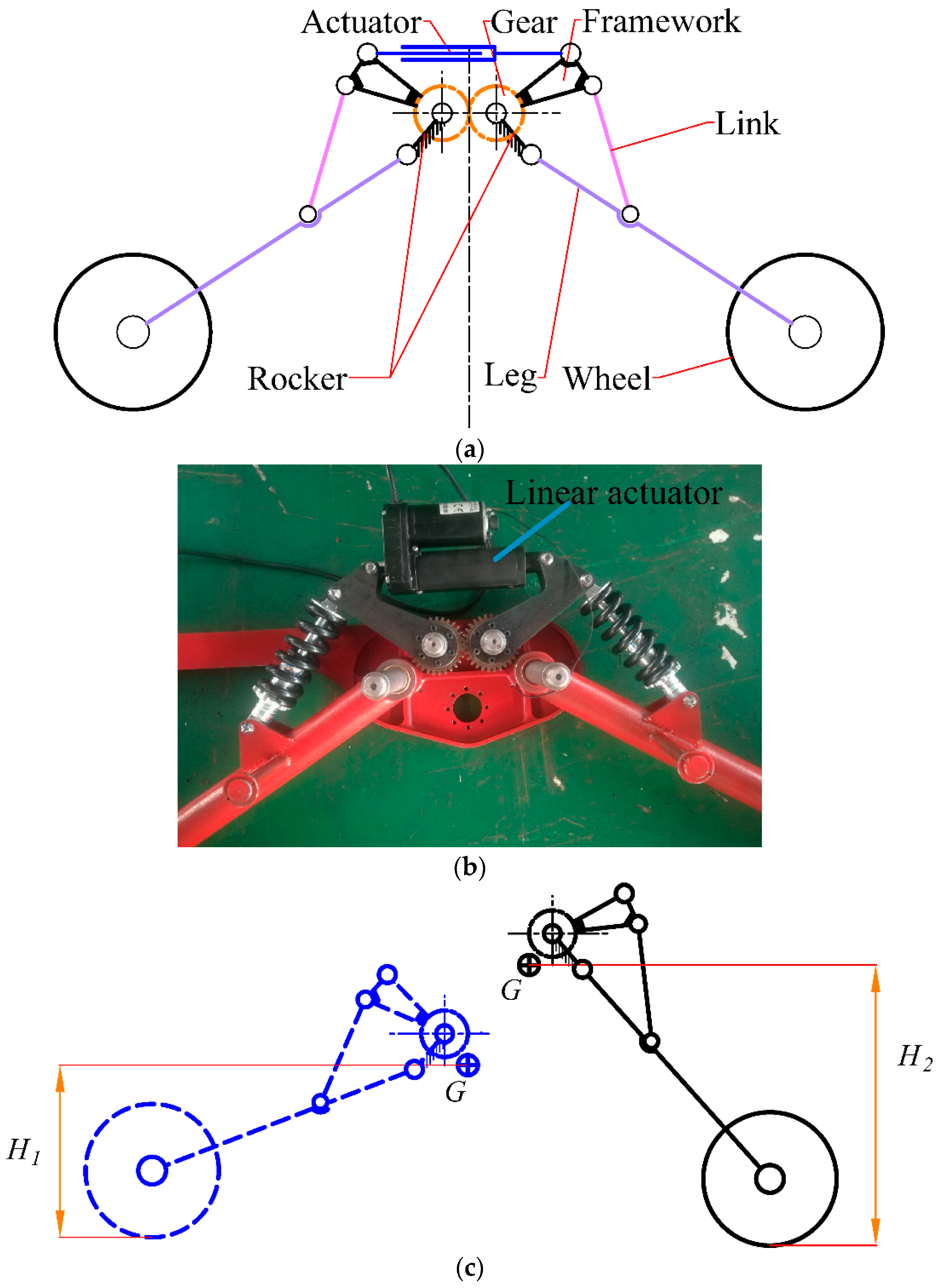
2.1. Concept of the Active Suspension

The concept of the novel active suspension was first proposal by Jiang et al. [27]. As shown in Figure 1, the active suspension is a type of symmetrical structure, in which each side is composed a gear, a framework, a link, a leg, and a wheel, respectively. The gear is fix-connected to the framework. Additionally, the gear ratio of this pair of driving gears is 1, ensuring that the motions between the left and right sides of the active suspension are coincident. Thus, the two legs can maintain an angular bisection rotation. By changing the input of the active suspension, a pair of gears are driven. Then, the height of each side can be actively adjusted.
In this paper, the active DoF (degree of freedom) is driven by a linear actuator. This linear actuator is a kind of electromotive handspike. The electromotive handspike is a displace implementing and position control mechanism for adjusting the state and control the system. In addition, the electromotive handspike is always self-locking during the process. As shown in Figure 1b, this electromotive handspike is a telescopic structure connecting the left and right sides of the active suspension, which is placed in the horizontal direction. Thus, the height of each side can be adjusted by controlling a linear actuator. Furthermore, the input (a linear actuator) is self-locking, and the robot with this active suspension can maintain its posture. The actuators only have to be driven when a change in the locomotion system is desired. Thus, the energy efficiency of wheeled locomotion is maintained.
In general, the height of each side can be changed via input to the active suspension (linear actuator length). There are three advantages of this suspension. (1) Two motor gears ensure that two legs can maintain their angular bisection rotation. The left and right frameworks are connected by a linear actuator. (2) The angle between each leg is adjusted by this actuator, facilitating a change in the height of each adjustable active suspension. Thus, this active suspension provides easy control for adjusting the robot’s attitude. (3) The positions of revolute joints in the active suspension are flexible [27].

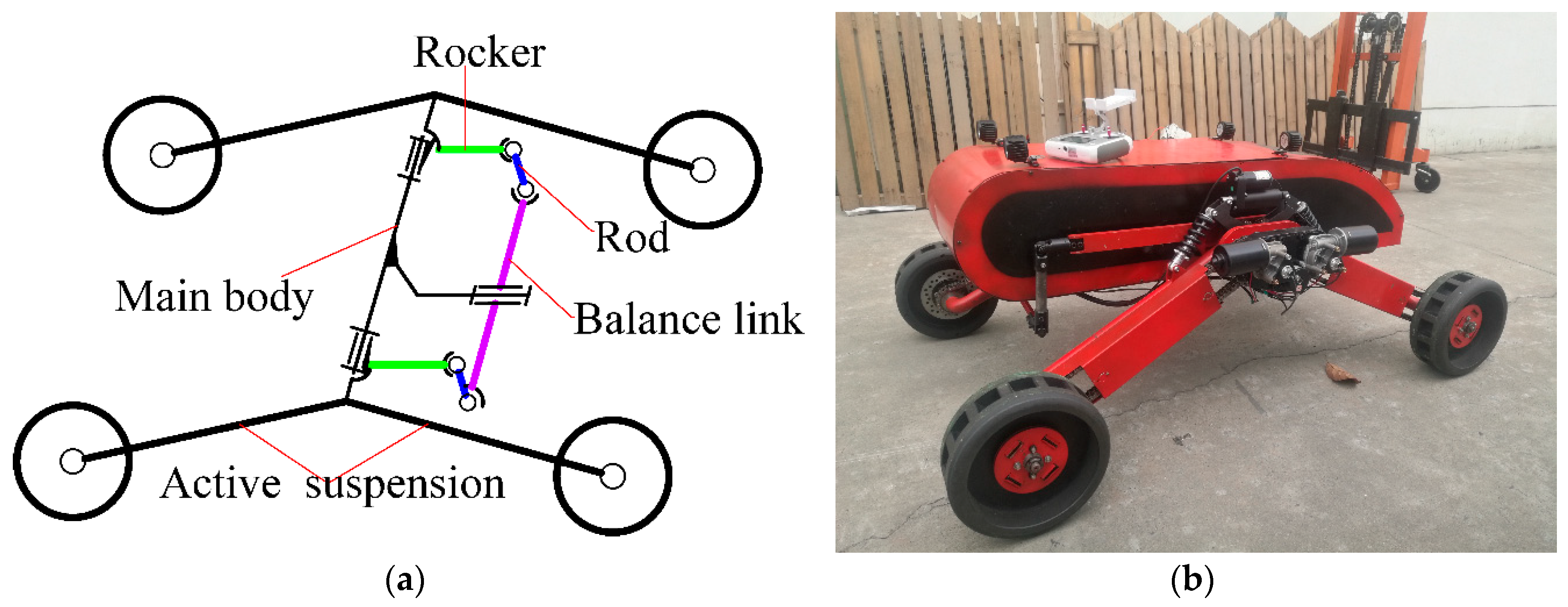
2.2. Mobile Robot with Active Suspension

As shown in Figure 2, this active suspension is mounted on the mobile robot by using a balance–rocker mechanism. The mobile robot has two active suspensions, a balance–rocker mechanism and a main body. As shown in Figure 2a, two rockers, two rods, and the balance-link comprise the balance–rocker mechanism. It uses a differencing linkage to ensure four-time four-wheel drive in a complex road environment while maintaining the main body at a constant level attitude in the angle bisector of the two active suspensions [28]. Another function supports the main body. With the balance–rocker mechanism, the robot can passively adapt to uneven terrain.
As shown in Figure 2, the mobile robot can actively reconfigure itself with the inputs of the left and right active adjustable suspensions. As referenced in Section 2.1, the height of each side can be changed in this way, via the length of the linear actuators. Thus, the mobile robot can actively reconfigure itself with the linear actuators in both sides. The mobile robot can be also controlled by changing the lengths of the left and right linear actuators. Additionally, the power requirements of reconfiguration are provided by the two electromotive handspikes, which act as the linear actuators. As shown in Figure 3a,b, when the inputs of the left and right active suspensions are equal, the ground clearance can be continuously and actively adjusted. As shown in Figure 3c, when the inputs of the left and right active suspensions differ, the roll angle of the robot can be actively adjusted to enhance the robot’s mobility.
Generally, a mobile robot can actively adjust its roll angle using its two side actuators, causing the lateral stability to improve.

3. Active Suspension’s Model

This study proposes a model that represents the relationship between the active input of a robot and its lateral stability. Consequently, two models are proposed: a complete active suspension model and a robot model. The former expresses the relationship between the input (i.e., configuration of the active suspension) and the output (i.e., center of gravity (COG) of the active suspension). The latter introduces lateral stability as a function of the positions of the COG on both sides. By combining these two models, a sufficient amount of stability is obtained for arbitrary robot configuration.
Firstly, the parameters of this suspension are designed. Based on the designed parameters, the relationship between the input (i.e., configuration of the active suspension) and the output (i.e., center of gravity (COG) of the active suspension) is achieved.

3.1. Parameters Design

In this section, we design the parameters of this active suspension. The aim of this section is to achieve the length ranges of the linear actuator when the structural parameters are given. As shown in Figure 4, the active suspension is symmetric. It comprises quadrangle E 1 E 2 B 2 B 1 , symmetric triangle EBD, and symmetric quadrangle ACBD. The parameters are defined as follows: E 2 B 2 B 1 = β 1 , EBD = β 2 , C 2 B 2 B 1 = β 3 , ACO = β 4 , DBC = α 1 , and ACB = π α 3 . The length of BD, AD, AC, BC, C 1 C 2 , B 1 B 2 , and EB are denoted by l 1 ,   l 2 ,   l 3 ,   l 4 ,   l 5 ,   l 6 , and l 7 , respectively.
Among the overall design of the mobile robot, ground clearance is an important index that can affect the mobility of this mobile robot. Thus, the input of the active suspension (length of the linear actuator) can be determined with the desired lowest and highest ground clearances. The min and max limited positions of the length of the linear actuator ( L e m i n   and   L e m a x ) correspond to the min and max ground clearances ( H C m i n   and   H C m a x ), respectively. As shown in Figure 4, the relationship between L e and H C is shown below:
H C = L 0 cos ( α 2 ) + R + H 3
where L 0 is the leg length, α is the two legs, including the angle, and H 3 is the vertical displacement between the ground clearance and the hinged point of the leg.
1. Solving α :
Solving Equation (1) leads to the following equation:
α ( H C ) = 2  *  arcos ( H C R H 3 L 0 ) .
2. Solving α 3 :
As shown in Figure 4, the relationship between α 3 and α can be written as follows:
α 3 ( H C ) = α ( H C ) 2 β 3 + β 4 + π 2 .
3. Solving α 1 :
As shown in Figure 4c, A C B D is a planar four-bar linkage, α 1 and α 3 are the input and output rotation angles, thus:
A cos α 1 + B sin α 1 + C = 0 ,
where:
{ A = l 3 cos α 3 + l 4 B = l 3 sin α 3 C = l 2 2 ( A ) 2 ( B ) 2 l 1 2 2 l 1 .
Thus:
α 1 ( H C ) = 2 arctg B ± ( A ) 2 + ( B ) 2 ( C ) 2 A C = u ( α 3 ( H C ) ) .
4. Solving L e :
The upper part of the active suspension is shown in Figure 4b. According to quadrangles E 1 E 2 B 2 B 1 and B 1 B 2 C 2 C 1 , which are all symmetric:
L e ( H C ) = 2 l 7 sin ( π β 2 α 1 ( H C ) arcsin ( l 5 l 6 2 l 4 ) ) + l 6 .
Thus, the length of the linear actuator L e can be achieved when the ground clearance ( H C ) is given with Equations (2)–(6), the relationship is described below:
L e = v ( H C ) ,
where L e is the length of the linear actuator, and H C is the ground clearance.
According to Equation (7), the min and max length of the linear actuator ( L e m i n and L e m a x ) can be achieved when the lowest and highest ground clearance are given, respectively.

3.2. Relationship between Input and Output

In this section, we describe the input–output relationship of the active suspension. As shown in Figure 4, the aim of this mechanism is to achieve the relationship between input ( L e ) and output (H). L e is the linear actuator length, and H is the height of the COG. Thus:
H ( L e ) = L 0 cos ( α 2 ) + R + H 2
where L 0 is the length of the leg, α is the included angle of two legs, and H 2 is the vertical displacement between the hinged point of the leg and the COG.
Hence, the entire equations to obtain the input–output relationship can be found in Appendix A [27], by substituting Equations (A2), (A4) and (A7) into Equation (8), the following deduction can be made:
H ( L e ) = L 0 cos ( w ( α 1 ( L e ) ) + arcsin ( l 5 l 6 2 l 4 ) + π 2 β 4 π 2 ) + R + H 2
Then, H is the function of independent variable ( L e ):
H = f ( L e )
Therefore, the relationship between the input (linear actuator length) and the output (COG) of the active suspension is given by Equation (10). Each active suspension can actively adjust its COG.

4. Lateral Stability

Stability is important for locomotion systems; it is the essential prerequisite for the robot to travel on unstructured terrain. Posture control in an articulated ground vehicle is a possible way to enhance the locomotion performance [17]. The mobile robot proposed here can adjust its roll angle by using its active suspension.
The purpose of this study is to propose a model that represents the relationship between the active input of a robot and its lateral stability. The kinematic model of the active suspension was established in Section 3. The relationship between the input, configuration, output, and COG of the active suspension is achieved. Therefore, we propose a mechanical model of a robot on a slope. A stability pyramid method is used to evaluate the robot’s stability. We make several assumptions to simplify the problem [22]:
  • The robot is equipped with four rigid wheels, driven independently.
  • The steering angle of each wheel is fixed at 0.
  • The robot travels along a flat side slope.
  • The traversing speed is low, and the motion of the robot remains in a steady state.

4.1. Corridinate Systems

Here, two coordinate systems (i.e., slope coordinate system and mobile robot coordinate system) are defined. Figure 5 illustrates a mobile robot laterally traversing a slope of angle θ . The mobile robot and its wheels are at a tilted angle, ψ h , against the slope, as shown in Figure 5, ψ h positively increases in the uphill direction. In Figure 5, the slope coordinate system, Σ s , is defined as follows: x ( s ) denotes the desired traversing direction, y ( s ) denotes the uphill direction, and z ( s ) denotes the vertically upward direction against the slope surface as a right-handed system. Then, the mobile robot system, Σ r , is obtained through a rotation of Σ s about the x ( s ) axis with ψ h in the uphill direction.

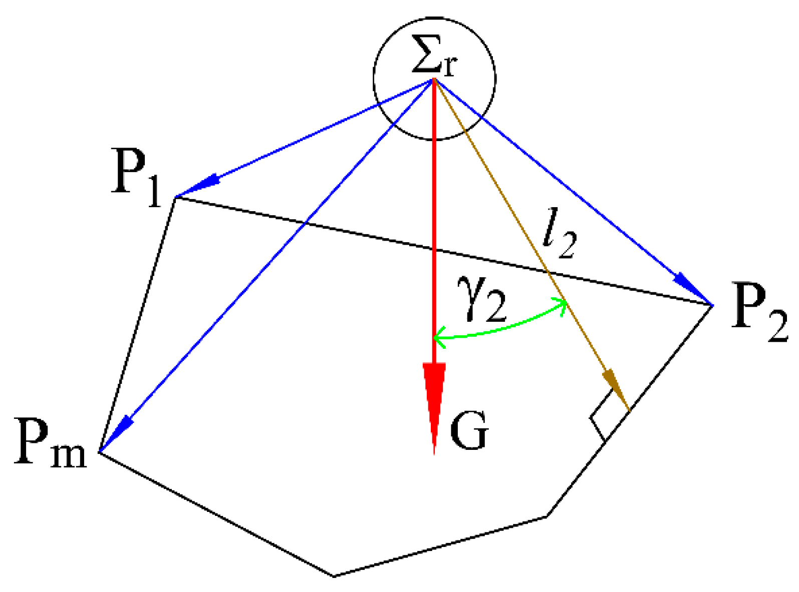
4.2. Define of Lateral Stability Parameters

For the mobile robot, we developed the criterion proposed in Papadopoulos and Rey [29]. As shown in Figure 6, the stability of the robot is evaluated with the gradient stability margin method [29], which can be summarized as follows. The line joining two consecutive terrain contacts, P i , defines a tip-over axis. The unit vector, l i , of the axis joining the robot COG, G , to the center of each tip-over axis is computed. Then, angle γ i , between each l i and the total force vector applied to the robot, gives the stability angle over the corresponding tip-over axis. The gradient, β , is the minimum angle, γ i , necessary to tip the mobile robot over.
β = min ( γ i ) .
Therefore, as shown in Figure 7, we can evaluate the lateral stability with the lateral tip-over gradients [30].
β l = min ( γ 1 , γ 2 )
β l denotes the lateral stability of the mobile robot. The larger the value of | β l | , the greater the lateral stability of the mobile robot over the terrain. Tip-over instability occurs for β l 0 .

4.3. Mechanical Model of a Reconfigurable Mobile Robot

In this section, we propose a mechanical model of a reconfigurable mobile robot on a slope. As shown in Figure 8, we assume that the COG of the mobile robot is located at distances L d and L u from the downhill and uphill wheels along the y ( r ) axis, respectively, and at distances H d and H u from those wheels along the z ( r ) axis. Here, both L d and L u are constant, whereas H d and H u vary with the input of the active suspension, which is obtained with Equation (10). We can actively adjust the inputs of the two active suspensions in both sides together. Then, both H d and H u are changed, and the roll angle of the robot adjusts. Overall, the mobile robot increases its lateral stability with the inputs of the two suspensions together.
As shown in Figure 8, θ denotes the roll angle of the mobile robot, and ψ h is the adjusted angle with regard to the slope. The mobile robot actively adjusts its roll on the slope. The expression of θ is:
{ Initial   state :   θ = θ   Reconfigure   state :   θ = θ ψ h
Therefore, the expressions of the lateral tip-over gradients γ i ( i = 1 , 2 ) are:
{ D o w n h i l l   s i d e :   tan ( γ 1 + θ ) = L d H d U p h i l l   s i d e :   tan ( γ 2 θ ) = L u H u
As shown in Figure 8, in the right-angled triangle, OP1P2, the adjustable angle of the mobile robot with regard to slope ψ h , is:
tan ( ψ h ) = H d H u L d + L u
where H d varies with the input of the downhill-side suspension, and H u varies with the input of the uphill-side suspension.
As referenced in Section 3, we denote L e u and L e d as the inputs of the active suspensions in the uphill and downhill sides, respectively. Putting L e u and L e d into Equation (10), we get:
{ D o w n h i l l   s i d e :   H d = f ( L e d ) U p h i l l   s i d e :   H u = f ( L e u )
By substituting Equations (13), (15) and (16) into Equation (14), solutions for lateral tip-over gradients are obtained employing the inputs, L e d and L e u , which are the lengths of downhill-side and uphill-side linear actuators, as variables.
• Initial state:
{ D o w n h i l l   s i d e :   λ 1 = arctan ( L d H d ) θ U p h i l l   s i d e :   λ 2 = arctan ( L u H u ) + θ
• Reconfigure state:
{ D o w n h i l l   s i d e :   λ 1 = arctan ( L d f ( L e d ) ) ( θ f ( L e d ) f ( L e u ) L u + L d )   U p h i l l   s i d e :   λ 2 = arctan ( L u f ( L e u ) ) + ( θ f ( L e d ) f ( L e u ) L u + L d )
Therefore, the lateral stability criteria, β l , is:
β l = min ( λ 1 , λ 2 ) = v ( L e u , L e d )
where L e d and L e u are the linear actuator lengths on the downhill and uphill sides, respectively, and θ is the slope angle.
Therefore, the lateral stability criteria, β l , can be obtained by employing the inputs L e u and L e d as variables.

5. Case Studies

5.1. Case Study of the Active Suspension

The case study of the active suspension is divided as the design and kinematic modeling.
Firstly, the design parameters of the active suspension are given. According to Equations (1)–(7) in Section 3.1, the ground clearance changes with the input of the active suspension (linear actuator length, L e ). The linear actuator’s min length L e m i n is achieved with the lowest ground clearance H C m i n ; meanwhile, L e m a x (the max length of the linear actuator) is achieved with H C m a x (the highest ground clearance). Table 1 shows the structure parameters of the active suspension used in the simulations, where, L 0 , l 7 l 7 , β 2 , and β 4 are cited from the reference [27]. R is the wheel’s radius; all the four wheels are the same. In addition, all the parameters listed in Table 1 can be measured from the UG/3D drawing software model. Calculations were done using MATLAB software.
The desired ground clearance of this mobile robot is from 350 mm to 550 mm. According to Equation (7) in Section 3.1, the min and max lengths of the linear actuator are solved as L e m i n = 170   m m , L e m a x = 221   m m . Thus, in order to choose a normal electromotive handspike, which can be provided easily, the min and max lengths are rounded as L e m i n = 170   m m , L e m a x = 220   m m . The change distance is 50 mm. Thus, the range of the linear actuator is:
170   m m L e 220   m m
Then, the goal of this section is to obtain the relationship between the input and output of the active suspension. The relationship between input L e (linear actuator length) and output H (height of COG) or ground clearance ( H C ) of the active suspension can be calculated using Equations (1) and (10) in Section 3, respectively. Figure 9 shows the relationship between the input and output of the active suspension. As indicated, both the ground clearance, H C and the height of the COG, H , increase with the increasing linear actuator length, L e , when it is at its minimum value of 170 mm, H is 453 mm, and H C is 348 mm. When L e is at its maximum value of 220 mm, H is 650 mm, H C is 545 mm, and the ground clearance increases by 197 mm.
Generally, the height of each side increases in direct proportion to the input of the increase of the active suspension.

5.2. Case Study for Lateral Stability

From the proposed models, we can obtain both the relationship between the input of an active suspension and the height of each side, with a relationship between the lateral stability parameters and the heights of both sides. Therefore, applying the kinematic model of the active suspension to the reconfigurable mobile robot, the relationship between the inputs of the mobile robot and its lateral stability can be numerically estimated (Equation (19)).
The active model can be shown as below:
L e d L e 0   or   L e u L e 0
where L e 0 is the initial length for both the downhill and uphill linear actuators, and L e d are L e u are the downhill and uphill-side linear actuators’ lengths, respectively.
  • When L e d = L e u < L e 0 , both the height of COG (center of gravity) and the ground clearance are lower than the initial condition.
  • When L e d = L e u > L e 0 , both the height of COG (center of gravity) and the ground clearance are higher than the initial condition.
  • When L e d L e u , the roll angle of the mobile robot is actively adjusted to enhance the stability of the mobile robot.
In the following subsections, various case studies are presented that demonstrate different adjustment models while performing lateral stability. The geometric parameters used in the case studies are listed in Table 2, which are from the reference [27].

5.2.1. Inputs of Uphill and Downhill Sides are Equal

When L e d = L e u L e 0 , the mobile robot can enhance its stability by changing the ground clearance. With the process of changing the ground clearance, the relationship between the length of the linear actuator and the lateral stability (Equation (19)) is shown in Figure 10. The roll angle of the slope was varied from 0° to 20° at 5° intervals.
Figure 10 shows the effect of the length of the linear actuator on mobile lateral stability responses. The lateral stability criteria, β l , exhibit a gradually varying linear growth tendency as the length of linear actuator decreases under different slope angles, and the ground clearance increases with the length of the linear actuator. Thus, the mobile robot is the most stable when it’s at its lowest ground clearance with the minimum value of the length of the linear actuator.

5.2.2. Inputs of Uphill and Downhill Sides are Unequal

According to the relationship between the ground clearance and the lateral stability in Section 5.2.1, the robot is most stable at its lowest ground clearance. When L e d L e u , the roll angle of the robot changes, the mode in this section is to extend the linear actuator on the downhill side. Specifically, the robot is at its lowest ground clearance in its initial state. Then, it adjusts its roll angle by expending the linear actuator on the downhill side. The roll angle of the slope was varied from 0° to 20° at 5° intervals.
The adjustment angle ( ψ h ) can be calculated using Equations (15)–(16). Figure 11a shows the relationship between the linear actuator length on the downhill side ( L e d ) and adjustment angle ( ψ h ). As indicated, the adjustment angle ( ψ h ) increases with the increasing linear actuator length on the downhill side ( L e d ). Its maximum is 12.33°. In other words, the mobile robot can level its configuration when the slope angle is lower than 12.33°.
The roll angle of the robot can be obtained using Equations (13), (15) and (16). As indicated in Figure 11b, when the slope angle is 5° or 10°, the roll angle of the robot decreases to 0°. Then, it increases in the inverse direction. When the slope angle is 15° or 20°, the roll angle of the robot decreases with the increasing linear actuator length on the downhill side ( L e d ).
The relationship between the lateral stability criteria ( β l ) and the linear actuator length on the downhill side ( L e d ) is shown in Figure 11c. When the slope angle is 5°, β l increases first, and then decreases. When the slope angle is 10°, 15°, or 20°, β l increases with L e d . Specifically, when the slope angle is 5°, as the linear actuator length on the downhill side ( L e d ) increases, the adjustment angle ( ψ h ) increases, and the roll angle of the robot ( θ ) first decreases, and then increases in the inverse direction. Referencing Equation (18), the lateral tip-over gradient on the downhill side ( λ 1 ) increases, and the lateral tip-over gradient on the uphill side ( λ 2 ) decreases; when λ 1 = λ 2 , β l obtains its maximum value (41°), it then decreases. When the slope angle is 10°, 15°, or 20°, as the linear actuator length on the downhill side ( L e d ) increases, the adjustment angle ( ψ h ) increases. Referencing Equation (18), the lateral tip-over gradient on the download side ( λ 1 ) increases constantly, and the lateral tip-over gradient on upload side ( λ 2 ) decreases constantly when L e d is at its maximum (220 mm) and β l reaches its maximum. By expending the linear actuator on the downhill side when the slope angle is 5°, β l increases from 39.78° to 41° (3.07%). When the slope angle is 10°, β l increases from 34.78° to 37° (6.38%). When the slope angle is 15°, β l increases from 29.78° to 32° (7.45%). When the slope angle is 20°, β l increases from 24.78° to 27° (8.96%).
Overall, the lateral stability criteria β l can be increased by expending the linear actuator on the downhill side ( L e d ) when the initial state of the robot is in its lowest ground clearance. Then, the lateral stability of the robot increases. Then, the lowest ground clearance is the most stable with respect to the other ground clearances, while referencing Section 5.2.1. Thus, the mobile robot can increase its lateral stability by adjusting the lengths of the linear actuators on both sides, no matter what the initial state of the robot is.

5.2.3. Leveled Configuration

The leveled configuration can also be adjusted, as shown in Figure 3c. The aim of this section is to compare the lateral stability of the initial state and leveled configuration. Specifically, the robot is at its lowest ground clearance in its initial state. Then, it adjusts its roll angle by expending the linear actuator on the downhill side.
The relationship between the lateral stability criteria ( β l ) and the slope angle is shown in Figure 12. Generally, the leveled configuration is more stable than the initial state. When the slope angle is 5°, β l increases from 39.78°to 40.22°(1.11%); when the slope angle is 10°, β l increases from 34.78° to 36.32°(4.43%); when the slope angle is 12°, β l increases from 32.78° to 34.91°(6.5%).

5.2.4. Discussion

The above results show that a mobile robot with an active suspension is able to increase its lateral stability by properly adjusting its configuration. More specifically, the configuration is changed by adjusting the linear actuator lengths on both the downhill and uphill sides.
When the linear actuator lengths on both sides are equal, the ground clearance and the lateral stability can be adjusted. The lowest ground clearance is the most stable with respect to others. In other words, the mobile robot is most stable when the linear actuator lengths on both sides are all at their minimum values. Then, for the initial state, the mobile robot is the most stable at its lowest ground clearance.
Thus, expending the linear actuator on the downhill side when the initial state is at its lowest ground clearance is chosen as the method. With the method, the robot increases its lateral stability, because the initial state at the lowest ground clearance is the most stable with respect to the other states. Thus, the robot’s configuration can enhance its lateral stability with an active suspension amid different ground clearances.
In addition, the leveled posture can be considered as an appropriate configuration, because the equipment on the robot can run smoothly with the level configuration. The mobile robot can level its configuration when the angle of the side slope is less than 12.33°. The leveled configuration is achieved during the process of the method (expending the linear actuator on the downhill side when the initial state is at its lowest ground clearance). During this process, the leveled attitude is not the configuration with maximum stability. Overall, the leveled configuration is a kind of posture that can both enable the robot work smoothly and increase the robot’s lateral stability, to some extent.

6. Manufacture and Test of a Prototype

A prototype mobile robot utilizing an active adjustable suspension is designed, as shown in Figure 2b. It is composed with the balance–rocker mechanism, main body, and two active suspensions on both sides. The robot can achieve basic functions, such as move forward, move back, and turn. Figure 13a shows that the robot overcomes a slope; Figure 13b shows the robot overcomes an obstacle unilaterally.
Some interesting tests are carried out to check the practical performances of the mobile robot. The robot can transform into two locomotion modes: the passive mode with a balance–rocker mechanism, and an active model with an active suspension. When the robot runs on rough and flat terrain, it usually works in the passive mode to achieve high velocity and an easy control system. When the robot encounters large obstacles or complicated terrains, it can transform itself from the passive model into the active mode. Then, the robot is consequently transformed into an active reconfiguration, which helps adapt itself to work on a complex terrain with high obstacles and steep slopes.
Furthermore, Figure 13c–e shows that the robot can actively adjust its configuration. Figure 13c,d shows the robot changes ground clearance with its own inputs (the length of linear actuator) from the lowest point to the highest point. Figure 13e shows that the robot can level itself over the scissors road. Generally, the robot can reconfigure itself in the field.
The test conducted with the physical prototype demonstrates that the prototype of the mobile robot utilizing an active adjustable suspension is successful.

7. Conclusions

We presented a mathematical model of a mobile robot using a novel active adjustable suspension system on side slopes. The relationship between the active inputs of the robot and the lateral stability was thus obtained. The following takeaways can be extracted from this article.
(1)
The ground clearance can be changed by the active suspension, and the robot is most stable at its lowest ground clearance. The height of the COG increases with the input of the active suspension (linear actuator length). When the linear actuator length varies from 170 to 220 mm, the height of the COG changes from 453 to 650 mm.
(2)
With an active suspension, the robot’s configuration can enhance lateral stability by changing the linear actuator lengths on both sides. When the robot is at its lowest ground clearance, the lateral stability criteria increases by expending the linear actuator on the downhill side. Thus, the robot can increase its lateral stability under different ground clearances. In addition, the robot can level itself when the angle of the side slope is less than 12.33°, and leveled posture can be considered as an appropriate configuration to enable the robot and its tools to work smoothly. Thus, the robot can be applied to agriculture, especially in hilly and mountainous terrains.
(3)
The mathematical model represents the relationship between the input (linear actuator lengths on both sides) and the output (stability), providing a theoretical basis for the design and control for mobile robots.

Author Contributions

G.X., F.G. and W.Z. conducted this study and proofread the manuscript together; H.J. conceived the idea, designed and analyzed the mobile robot with an active suspension, and wrote this manuscript; W.Z. and K.C. contributed to the practical model for the mobile robot, and proofread the manuscript.

Funding

This research was funded in part by the National Natural Science Foundation of China under grant numbers 51675027 and 51775016, and in part by the National Key Technology R&D Program of China under grant number 2016YFD0700503-1.

Conflicts of Interest

The authors declare no conflict of interest.

Appendix A. Proof of the Relationship between L e and α in the Active Suspension

This section is the kinematic model of the active suspension with regard to the relationship between L e (length of the linear actuator) and α (the two legs, including the angle).
1. Isosceles trapezoid E 1 E 2 B 2 B 1 :
β 1 = arcsin ( L e l 6 2 l 7 ) + π 2 .
2. Isosceles trapezoid B 1 B 2 C 2 C 1 :
β 3 = arcsin ( l 5 l 6 2 l 4 ) + π 2
3. Solving α 1 :
Figure 4b shows the upper part of the active suspension.
β 1 + β 2 + β 3 + α 1 = 2 π
Substituting Equations (A1) and (A2) into Equation (A3) leads to the following equation:
α 1 = π arcsin ( L e l 6 2 l 7 ) arcsin ( l 5 l 6 2 l 4 ) β 2
where L e is actively adjustable. The other parameters are determined by the structure of the active suspension.
4. A planar four-bar mechanism, ACBD:
Figure 4c shows a planar four-bar mechanism, ACBD. The closed loop equation is:
{ l 1 cos α 1 + l 2 cos α 2 = l 4 + l 3 cos α 3 l 1 sin α 1 + l 2 sin α 2 = l 3 sin α 3
Equation (A5) can be rewritten by eliminating α 2 , as follows:
Acos α 3 + Bsin α 3 + C = 0 ,
where:
{ A = l 4 l 1 cos α 1 B = l 1 s i n α 1 C = A 2 + B 2 + ( l 3 ) 2 ( l 2 ) 2 2 l 6
Then:
α 3 = 2 arctan B ± A 2 + B 2 C 2 A C = w ( α 1 )
5. Solving for α :
α = 2 ( α 3 + β 3 β 4 π 2 )

References

  1. Bruzzone, L.; Quaglia, G. Locomotion systems for ground mobile robots in unstructured environments. Mech. Sci. 2012, 3, 49–62. [Google Scholar] [CrossRef]
  2. Tarokh, M.; Ho, H.D.; Bouloubasis, A. Systematic kinematics analysis and balance control of high mobility rovers over rough terrain. Robot. Auton. Syst. 2013, 61, 13–24. [Google Scholar] [CrossRef]
  3. Luo, Z.; Shang, J.; Wei, G.; Ren, L. A reconfigurable hybrid wheel-track mobile robot based on Watt II six-bar linkage. Mech. Mach. Theory 2018, 128, 16–32. [Google Scholar] [CrossRef] [Green Version]
  4. Iagnemma, K.; Rzepniewski, A.; Dubowsky, S.; Schenker, P. Control of robotic vehicles with actively articulated suspensions in rough terrain. Auton. Robot 2003, 14, 5–16. [Google Scholar] [CrossRef]
  5. Li, Z.; Ma, S.; Li, B.; Wang, M.; Wang, Y. Analysis of the constraint relation between ground and self-adaptive mobile mechanism of a transformable wheel-track robot. Sci. China Technol. Sci. 2011, 54, 610–624. [Google Scholar] [CrossRef] [Green Version]
  6. Zhu, Y.; Fei, Y.; Xu, H. Stability Analysis of a Wheel-Track-Leg Hybrid Mobile Robot. J. Intell. Robot Syst. 2018, 91, 1–14. [Google Scholar] [CrossRef]
  7. Kim, D.; Hong, H.; Kim, H.S.; Kim, J. Optimal design and kinetic analysis of a stair-climbing mobile robot with rocker-bogie mechanism. Mech. Mach. Theory 2012, 50, 90–108. [Google Scholar] [CrossRef]
  8. Iagnemma, K.D.; Rzepniewski, A.; Dubowsky, S.; Pirjanian, P.; Huntsberger, T.L.; Schenker, P.S. Mobile robot kinematic reconfigurability for rough terrain. In Sensor Fusion and Decentralized Control in Robotic Systems III. International Society for Optics and Photonics; Boston, M.A., Ed.; SPIE: Bellingham, WA, USA, 2000; Volume 4196, pp. 413–421. [Google Scholar] [CrossRef]
  9. Wettergreen, D.; Moreland, S.; Skonieczny, K.; Jonak, D.; Kohanbash, D.; Teza, J. Design and field experimentation of a prototype lunar prospector. Int. J. Robot Res. 2010, 29, 1550–1564. [Google Scholar] [CrossRef]
  10. Wilcox, B.H.; Litwin, T.; Biesiadecki, J.; Matthews, J.; Heverly, M.; Morrison, J.; Townsend, J.; Ahmad, N.; Sirota, A.; Cooper, B. ATHLETE: A cargo handling and manipulation robot for the moon. J. Field. Robot 2007, 24, 421–434. [Google Scholar] [CrossRef]
  11. Aoki, T.; Murayama, Y.; Hirose, S. Development of a Transformable Three-wheeled Lunar Rover: Tri-Star IV. J. Field Robot 2014, 31, 206–223. [Google Scholar] [CrossRef]
  12. Cordes, F.; Dettmann, A.; Kirchner, F. Locomotion modes for a hybrid wheeled-leg planetary rover. In Proceedings of the 2011 IEEE International Conference on Robotics and Biomimetics (ROBIO), Karon Beach, Phuket, Thailand, 7–11 December 2011; pp. 2586–2592. [Google Scholar] [CrossRef]
  13. Halme, A.; Leppänen, I.; Salmi, S.; Ylönen, S. Hybrid locomotion of a wheel-legged machine. In Proceedings of the 3rd International Conference on Climbing and Walking Robots (CLAWAR’00), Madrid, Spain, 2–4 October 2000. [Google Scholar]
  14. Michaud, F.; Létourneau, D.; Arsenault, M.; Bergeron, Y.; Cadrin, R.; Gagnon, F.; Legault, M.-A.; Millette, M.; Pare, J.-F.; Tremblay, M.-C.; et al. AZIMUT, a leg-track-wheel robot. In Proceedings of the 2003 IEEE/RSJ International Conference on Intelligent Robots and Systems (IROS 2003), Las Vegas, NV, USA, 27–31 October 2003; pp. 2553–2558. [Google Scholar] [CrossRef]
  15. Edwin, L.E.; Denhart, J.D.; Gemmer, T.R.; Ferguson, S.M.; Mazzoleni, A.P. Performance Analysis and Technical Feasibility Assessment of a Transforming Roving-Rolling Explorer Rover for Mars Exploration. J. Mech. Des. 2014, 136, 071010. [Google Scholar] [CrossRef]
  16. Edwin, L.; Mazzoleni, A.; Gemmer, T.; Ferguson, S. Modeling, construction and experimental validation of actuated rolling dynamics of the cylindrical Transforming Roving-Rolling Explorer (TRREx). Acta Astronaut. 2017, 132, 43–53. [Google Scholar] [CrossRef]
  17. Grand, C.; Benamar, F.; Plumet, F.; Bidaud, P. Stability and traction optimization of a reconfigurable wheel-legged robot. Int. J. Robot Res 2004, 23, 1041–1058. [Google Scholar] [CrossRef]
  18. Zheng, J.; Gao, H.; Yuan, B.; Liu, Z.; Yu, H.; Ding, L.; Deng, Z. Design and terramechanics analysis of a Mars rover utilising active suspension. Mech. Mach. Theory 2018, 128, 125–149. [Google Scholar] [CrossRef]
  19. Besseron, G.; Grand, C.; Amar, F.B.; Bidaud, P. Decoupled control of the high mobility robot hylos based on a dynamic stability margin. In Proceedings of the 2008 IEEE/RSJ International Conference on Intelligent Robots and Systems, Nice, France, 22–26 September 2008; pp. 2435–2440. [Google Scholar] [CrossRef]
  20. Kubota, T.; Naiki, T. Novel mobility system with active suspension for planetary surface exploration. In Proceedings of the 2011 IEEE Aerospace Conference, Big Sky, MT, USA, 5–12 March 2011; pp. 1–9. [Google Scholar] [CrossRef]
  21. Chen, F.; Genta, G. Dynamic modeling of wheeled planetary rovers: A model based on the pseudo-coordiates approach. Acta Astronaut. 2012, 81, 288–305. [Google Scholar] [CrossRef]
  22. Inotsume, H.; Sutoh, M.; Nagaoka, K.; Nagatani, K.; Yoshida, K. Modeling, analysis, and control of an actively reconfigurable planetary rover for traversing slopes covered with loose soil. J. Field Robot 2013, 30, 875–896. [Google Scholar] [CrossRef]
  23. Inotsume, H.; Sutoh, M.; Nagaoka, K.; Nagatani, K.; Yoshida, K. Slope traversability analysis of reconfigurable planetary rovers. In Proceedings of the 2012 IEEE/RSJ International Conference on Intelligent Robots and Systems, Vilamoura, Portugal, 7–12 October 2012; pp. 4470–4476. [Google Scholar] [CrossRef]
  24. Gao, Q.M.; Gao, F.; Zhou, W.H. Stability analysis of hilly power platform with balance rocker suspension. Trans. CSAM 2013, 44, 291–293. [Google Scholar]
  25. Gao, Q.; Gao, F.; Tian, L.; Li, L.; Ding, N.; Xu, G.; Jiang, D. Design and development of a variable ground clearance, variable wheel track self-leveling hillside vehicle power chassis (V2-HVPC). J. Terramech. 2014, 56, 77–90. [Google Scholar] [CrossRef]
  26. Wang, Y.; Yang, F.; Pan, G.; Liu, H.; Liu, Z.; Zhang, J. Design and Testing of a Small Remote-Control Hillside Tractor. Trans. ASABE 2014, 57, 363–370. [Google Scholar] [CrossRef]
  27. Jiang, H.; Xu, G.; Zeng, W.; Gao, F. Design and kinematic modeling of a passively-actively transformable mobile robot. Mech. Mach. Theory 2019, 142, 103591. [Google Scholar] [CrossRef]
  28. Liu, B.; Gao, F.; Jiang, H.; Zhang, B. Attitude control algorithm of balancing-arm mobile robot. J. Beijing Univ. Aeronaut. Astronaut. 2018, 44, 391–398. [Google Scholar] [CrossRef]
  29. Papadopoulos, E.G.; Rey, D.A. A new measure of tipover stability margin for mobile manipulators. In Proceedings of the IEEE International Conference on Robotics and Automation, Minneapolis, MN, USA, 22–28 April 1996; Volume 4, pp. 3111–3116. [Google Scholar] [CrossRef]
  30. Freitas, G.; Gleizer, G.; Lizarralde, F.; Hsu, L.; dos Reis, N.R.S. Kinematic reconfigurability control for an environmental mobile robot operating in the amazon rain forest. J. Field Robot 2009, 27, 1340–1345. [Google Scholar] [CrossRef]
Figure 1. Active suspension: (a) Simple model; (b) Practical model; (c) Principle schematic.
Applsci 09 04410 g001
Figure 2. Mobile robot: (a) Simple model; (b) Practical model.
Applsci 09 04410 g002
Figure 3. Mobile robot reconfigurations: (a) Low ground clearance; (b) High ground clearance; (c) Leveled configuration.
Applsci 09 04410 g003
Figure 4. Parameter model of active suspension: (a) Whole; (b) Upper part; (c) Four-bar linkage.
Applsci 09 04410 g004
Figure 5. Definition of coordinate systems.
Applsci 09 04410 g005
Figure 6. Robot tip-over angles.
Applsci 09 04410 g006
Figure 7. Lateral stability margins for the robot.
Applsci 09 04410 g007
Figure 8. Mechanical mobile robot on a side slope.
Applsci 09 04410 g008
Figure 9. Input–output of the active suspension.
Applsci 09 04410 g009
Figure 10. Inputs on mobile robot stability responses.
Applsci 09 04410 g010
Figure 11. Lateral stability with expending the downhill side actuator: (a) Adjustable angle; (b) Roll angle; (c) Lateral stability criteria.
Applsci 09 04410 g011aApplsci 09 04410 g011b
Figure 12. Lateral stability of leveled configuration.
Applsci 09 04410 g012
Figure 13. Basic field experiments illustration: (a) Slope; (b) Unilateral obstacle; (c) Low ground clearance; (d) High ground clearance; (e) Leveled attitude.
Applsci 09 04410 g013aApplsci 09 04410 g013b
Table 1. Parameters of the active suspension.
ParameterValueUnitParameterValueUnit
L 0 640mm l 1 116.8mm
l 2 160mm l 3 161.1mm
l 4 52.1mm l 5 140.3mm
l 6 58mm l 7 103.1mm
R 150mm H 2 20mm
H 3 −85.5mm β 2 23.6°
β 4 16.9°
Table 2. Parameters of the mobile robot.
ParameterValueParameterValue
L d / mm 450 L u / mm 450

