Article

Aerodynamic Damping Prediction for Turbomachinery Based on Fluid-Structure Interaction with Modal Excitation

1
School of Energy and Power Engineering, Beihang University, Beijing 100191, China
2
Beijing Aerospace Technology Institute, Beijing 100074, China
3
Beijing Power Machinery Institute, Beijing 100074, China
*
Author to whom correspondence should be addressed.
Appl. Sci. 2019, 9(20), 4411; https://doi.org/10.3390/app9204411
Submission received: 4 July 2019 / Revised: 15 October 2019 / Accepted: 15 October 2019 / Published: 18 October 2019

Abstract

:
Aerodynamic damping predictions are critical when analyzing aeroelastic stability. A novel method has been developed to predict aerodynamic damping by employing two single time-domain simulations, specifically, one with the blade impulsed naturally in a vacuum and one with the blade impulsed in flow. The focus is on the aerodynamic damping prediction using modal excitation and the logarithmic decrement theory. The method is demonstrated by considering the first two bending modes with an inter-blade phase angle (IBPA) of 0° on a transonic compressor. The results show that the flutter boundary prediction is basically consistent with the experiment. The aerodynamic damping prediction with an IBPA of 180° is also performed, demonstrating that the method is suitable for different traveling wave mode representations. Furthermore, the influence of the amplitude of modal excitation and mechanical damping using the Rayleigh damping model for aerodynamic damping was also investigated by employing fluid-structure coupled simulations.

1. Introduction

Flutter has gradually become one of the most critical factors affecting turbomachinery reliability as technology has advanced recently (higher pressure ratio, thinner blade, etc.) [1]. Due to the high cost and time requirements of flutter experiments, accurate numerical flutter prediction methods are indispensable in the development of high-performance turbomachinery with wide flutter margins [2].
In turbomachinery, the traveling wave model, which was developed by Lane, is generally used for flutter predictions [3]. This model supposes that the blades in a rotor row vibrate with a constant inter-blade phase angle (IBPA) and frequency. It was first employed in flutter predictions by Carta [4], and subsequently named as an energy method by Bendiksen [5]. Due to its clear physical implications, it is widely used in numerical blade flutter analysis and design optimization [6,7,8]. In this way, the aeroelastic stability of a blade is revealed by aerodynamic damping, which is calculated using the unsteady aerodynamic work integrated into one vibration period with natural frequencies.
General flutter analysis methods, including the energy method, are concerned with the effects of flow on the surrounding structure, and vice versa. The flow and structure behave as a single system, an idea which is based on the small fluid-structure coupling assumption, which is often adequate when only considering the onset of flutter. Furthermore, nonlinear flutter behavior, such as limit-cycle oscillation (LCO), is unpredictable unless the full aeroelastic system is solved, including the flow and structural equations. For the coupled approach, the simultaneous integration of the Navier-Stokes equation and the structure’s motion in time allows for the accurate assessment of energy exchange between the fluid and the blade structure. Sisto et al. [9] applied a coupled method to study stall flutter in a linear cascade. A vortex and boundary layer method was used for incompressible flow, coupled with a spring model for the blade’s motion. A similar structure model was used by Hwang and Fang [10] to study the stall flutter of a transonic cascade. Sadeghi and Liu [11] solved the Euler and Navier-Stokes equations using a transonic cascade coupled with a linear-spring structure model. The coupled results showed strong nonlinear effects for a range of mass flow rates, which was significantly different from results obtained by conventional energy methods. In addition, the effects of frequency mistuning on cascade flutter were studied using this coupled method in their following paper [12]. Zheng and Yang [13] proposed a time-domain coupled fluid-structure method and applied it to the flutter analysis of Rotor 67. Debrabandere et al. [14] and Zhang et al. [15] adopted a two-way fluid-structure coupled method for aeroelastic analysis of a transonic axial compressor. The results showed that the blade vibration frequency deviated from the natural frequency due to the coupled influence. Cheng and Madsen et al. [16] applied fully coupled aero-hydro-servo-elastic time domain simulations to investigate the aerodynamic damping of a floating vertical axis wind turbine, which found the aerodynamic damping was almost independent of the rotor azimuth angle.
In turbomachinery, a coupled fluid-structure analysis for flutter represents the actual physical processes more closely rather than separated fluid and structural models. In the decoupled method, flutter stability is determined by unsteady aerodynamic work on a given rotor blade during an oscillating cycle. However, in the coupled fluid-structure method, the unsteady aerodynamic work usually converges to zero if vibration is stable. Thus, the time-domain fluid–structure coupled method is often only employed to predict the onset of flutter. Aerodynamic damping calculation methods for coupled fluid-structure method are essential to quantify the flutter margin of turbomachinery. Gottfried and Fleeter [17] developed an approach to predict aerodynamic damping with the fluid-structure coupled method and demonstrated it by using a transonic compressor. The same finite element model was applied to both the Euler and structural equations. Unfortunately, only the behaviors of the first bending and first torsion modes were determined by the blade’s simple impulse. Also, the interaction between the blades could not be taken into account, which is problematic considering that this is as a key factor affecting the aeroelastic stability.
In this paper, an aerodynamic damping prediction method based on a time-domain coupled fluid-structure method with modal excitation is developed, and a logarithmic decrement method for damped vibration is employed. In the coupled fluid-structure model, the Navier-Stokes and transient structure equations are processed simultaneously using the Raleigh damping model. The aerodynamic damping computation approach is performed on a transonic compressor flutter test rotor, BF_1_2 [18].

2. Numerical Methods

2.1. Fluid Dynamics

The commercial package ANSYS-CFX17.2 is used for the fluid simulation. Reynolds-averaged Navier-Stokes equations are employed to describe the physics of unsteady, compressible, viscous 3D flow [19]. Equation (1) includes the Reynolds-averaged continuity equation, momentum equation, and energy equation.
{ ρ t + x j ( ρ U j ) = 0 t ( ρ U i ) + x j ( ρ U i U j ) = P x i + x j ( τ i j ρ u i u j ¯ ) + S M t ( ρ h t o t ) P t + x j ( ρ U j h t o t ) = x j ( λ T x j ρ u j h ¯ ) + x j [ U i ( τ i j ρ u i u j ¯ ) ] + S E ,
where t is time, ρ is density, U is the average component of velocity, x is the displacement, P is pressure, τ is the molecular stress tensor (including both the normal and shear components of stress), u is the time varying component of velocity, ρ u i u j ¯ is the Reynolds stresses, S M is the momentum source term, T is temperature, S E is the energy source term, and h t o t is the mean total enthalpy, which is defined by the expression below:
h t o t = h + 1 2 U i U i + k ,
where k is the turbulent kinetic energy, given by:
k = 1 2 u i 2 ¯ .
The boundary conditions of the fluid domain on the fluid-structure interface are represented by Equation (4):
d f = d s ,
where d is the node displacement on the fluid-structure interface, the subscript f represents the fluid domain, and the subscript s represents the solid domain. The variable transferred from the solid domain to the fluid domain through the fluid-structure interface is the node displacement.
Spatial and temporal discretization are based on a second-order upwind difference scheme and a second-order backward Euler scheme, respectively. In addition, the k-ε turbulence model and scalable wall functions are employed for the wall treatment.

2.2. Structural Dynamics

Simultaneously, the commercial package ANSYS 17.2 is used for structural simulation. Structural elastic equations in matrix form are defined as:
{ [ A ] { σ } + { F } = 0 { ε } = [ A ] T { v } { σ } = [ D ] { ε } ,
where [ A ] is the differential operator, { σ } is tress, { F } is body force, { ε } is strain, { v } is the nodal displacement, [ D ] is the elastic matrix. The boundary conditions of solid domain on the fluid-structure interface are defined as Equation (6):
σ s n s = σ f n f ,
where σ s is the stress on solid domain side, σ f is the stress on fluid domain side, n is the normal vector. The aerodynamic load is transferred from the fluid domain across the fluid-structure interface.
Transient structural equations of the mechanical system with finite degrees of freedom are expressed below:
M x ¨ + C x ˙ + K x = F ,
where M is the mass matrix, C is the damping matrix, K is the stiffness matrix, x is the vector of displacements, and F is the external force vector. In this study, the Rayleigh damping model is employed to define mechanical damping. According to the definition of the Rayleigh damping model [19], the damping matrix C can be defined using Equation (8):
C = α M + β K ,
where the Rayleigh damping constants α and β are the mass damping constant and stiffness damping constant, respectively, which agree with the relationship defined in Equation (9):
ζ k = α 2 ω k + β ω k 2 ,
where ω k is the circle frequency of the kth natural mode and ζ k denotes the kth modal damping ratio of the material of the blade.
The Rayleigh damping constants α and β can be calculated by Equation (10) and Equation (11) from a considered frequency range of f l o to f u p , where ζ is considered a constant and f l o and f u p are the lowest and highest frequencies, respectively:
α = 4 π ζ f l o · f u p f l o + f u p ,
β = ζ π ( f l o + f u p ) β = ζ π ( f l o + f u p ) .

2.3. Fluid-Structure Interaction

The two-way coupled, partitioned fluid-solid interaction algorithm [19] is applied to simulate the flow-induced vibration of blade. The algorithm schematic is shown in Figure 1.
Within each real timestep, the flow equations and the structural equations are calculated simultaneously and information is exchanged on the fluid-structure interface. This procedure is repeated until the flow and displacements and the data exchanged on the interface are converged, before proceeding to the next timestep. On the fluid-structure interface, the coupling conditions represented by the boundary conditions in Equations (4) and (6) between the fluid and the structure needed to be satisfied [19].

2.4. Damping Calculation Method

The blade deviates from its equilibrium position when the impulse acts on its surface, and the vibration continues until the energy decays to zero. Damping is calculated using the logarithmic de-cay rates extracted from the time history of the blade displacement response. In the vacuum, the blade vibration always decays with time due to the mechanical damping. In the fluid, the coupled fluid-structure method is used to achieve a blade displacement response, which will diverge due to the summation of the unsteady aerodynamic work on the blade being larger than that of the mechanical dissipation. Otherwise, the blade displacement tends to converge. The logarithmic decrement of the amplitude of the blade’s vibration resulting from the damped vibration is shown in Figure 2; see [20] for further detail.
In this study, the behaviors of the different natural blade modes are determined by the artificial excitation force, which is distributed over the blade nodes and applied for a short time. The blade structural equations are defined in Equation (12), which is applicable when the excitation force is loaded onto the blade:
M x ¨ + C x ˙ + K x = F a + F e ,
where F a is the aerodynamic force transferred from the fluid domain in the CFX through the fluid-structure interface and F e is the excitation force, which can be expressed by the natural blade modes, as shown in Equation (13):
F e i = { k = 1 M A k   ( ψ k ) i sin ( 2 π f k t + φ k 0 ) 0 < t < T f 0 t T f ,
where t represents real time, T f is the excitation time of the blade, F e i is the excitation force on the i-th node, A k is the excitation force amplitude of the kth natural mode, ψ k is the normalized mode of the kth natural mode, ( ψ k ) i is the vibration displacement of the i-th node according to the normalized mode of the kth natural mode, f k is the natural frequency of the k-th mode, φ k 0 is the phase of the excitation force, and M is the concerned mode number.
The parameters in Equation (13) are adjusted to obtain arbitrary natural vibration modes, and the non-zero inter-blade phase angle is achieved by setting different phases of the excitation force on different blades. Curves of the excitation force acting on the tip leading-edge with IBPAs of 0° and 180° are shown in Figure 3a,b, respectively.
The blades vibrate with a certain natural mode and IBPA with a specific excitation force. After the excitation is removed, the damping is calculated using the decay rates extracted from the time history of the blade displacement response, as illustrated in Figure 2.

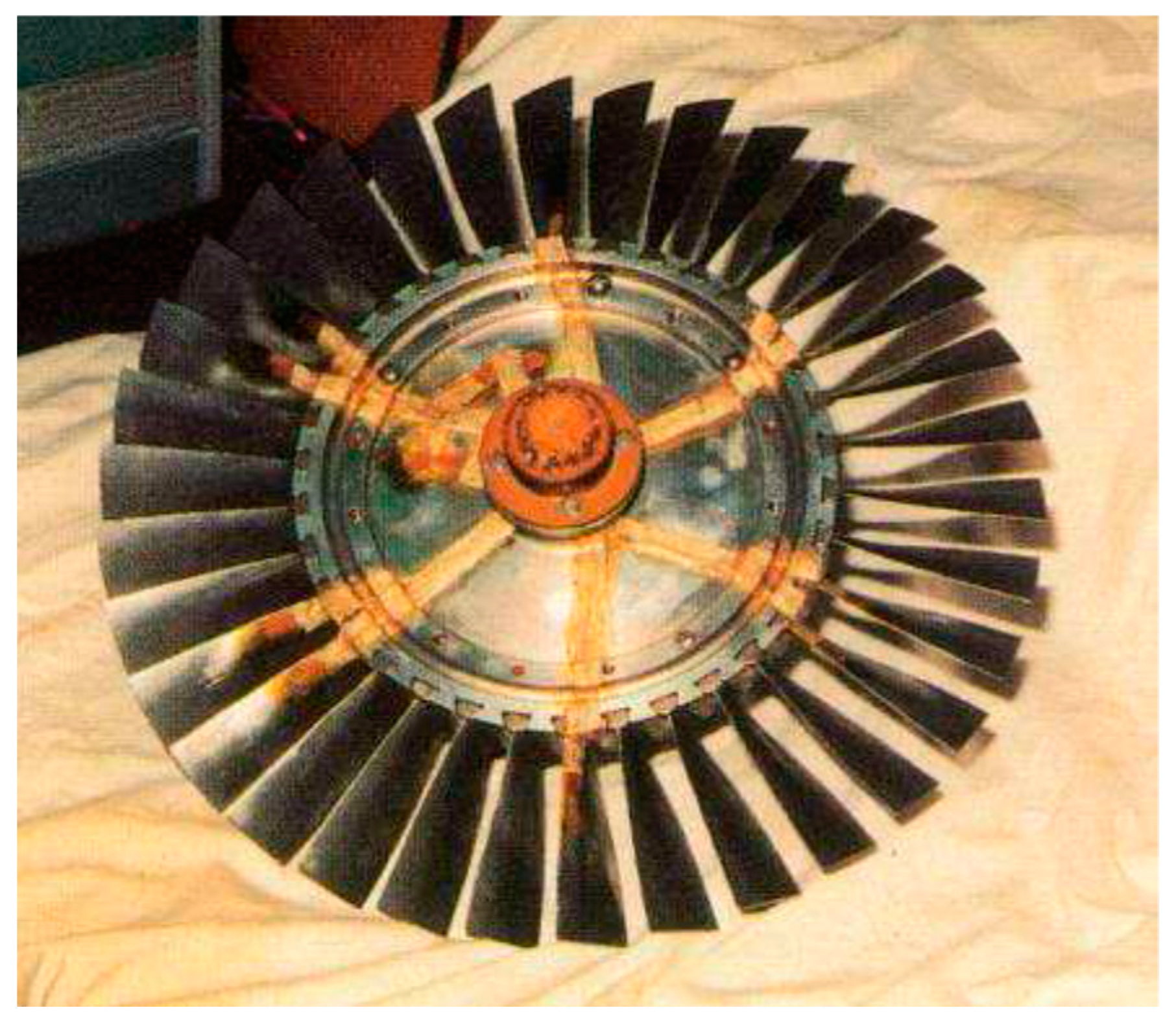
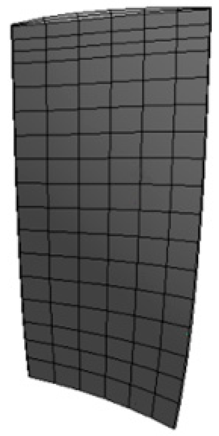
3. Computation Models

The compressor rotor named BF_1_2 is chosen to demonstrate the applicability of the numerical prediction method for aerodynamic damping. The main aerodynamic parameters are presented in Table 1. Figure 4 shows a picture of the testing rotor. Full details are given in [18].
Mode analysis is necessary to define the excitation force before the coupled fluid-structure simulation. The analysis finite element (FE) model is shown in Figure 5; the material is steel, and its main properties are shown in Table 2.
Figure 6 shows the computational fluid dynamics (CFD) model used for the Navier-Stokes computations. Based on the CFD and FE models, the aerodynamic damping prediction method with an IBPA of 0° for different natural modes is detailed. The double passage models are employed to elaborate on the aerodynamic damping prediction method for an IBPA of 180°.
The convergence criteria for the fluid analysis inside a stagger iteration in CFX require that the root mean square of the residuals of the mass and momentum is within 2 × 10⁻⁵. The convergence criteria for the transient structure analysis inside a stagger iteration in ANSYS require that the L2 norm of force is within 0.5%. And the convergence criteria for the stagger iteration require that residuals of all the data that exchanged on the interface are within 0.01. The timestep of the analysis is set to 1.0695 × 10⁻⁵ s.

4. Results and Discussion

The rotor aerodynamic performances at different speeds and blade modes are analyzed, and the numerical results are compared with the experimental results reported in [18]. A novel approach is detailed to predict the aerodynamic damping for different vibration modes. Two time-domain simulations are employed, specifically, one with the blade vibrating in a vacuum and another with the blade vibrating in flow. The effects of the Rayleigh damping and the amplitude of excitation with respect to the blade displacement response, as well as aerodynamic damping, are discussed respectively. The influence of the nonlinear fluid dynamics on aeroelastic stability is demonstrated as well. Finally, the applicability of the method for dealing with non-zero IBPA cases is illustrated.

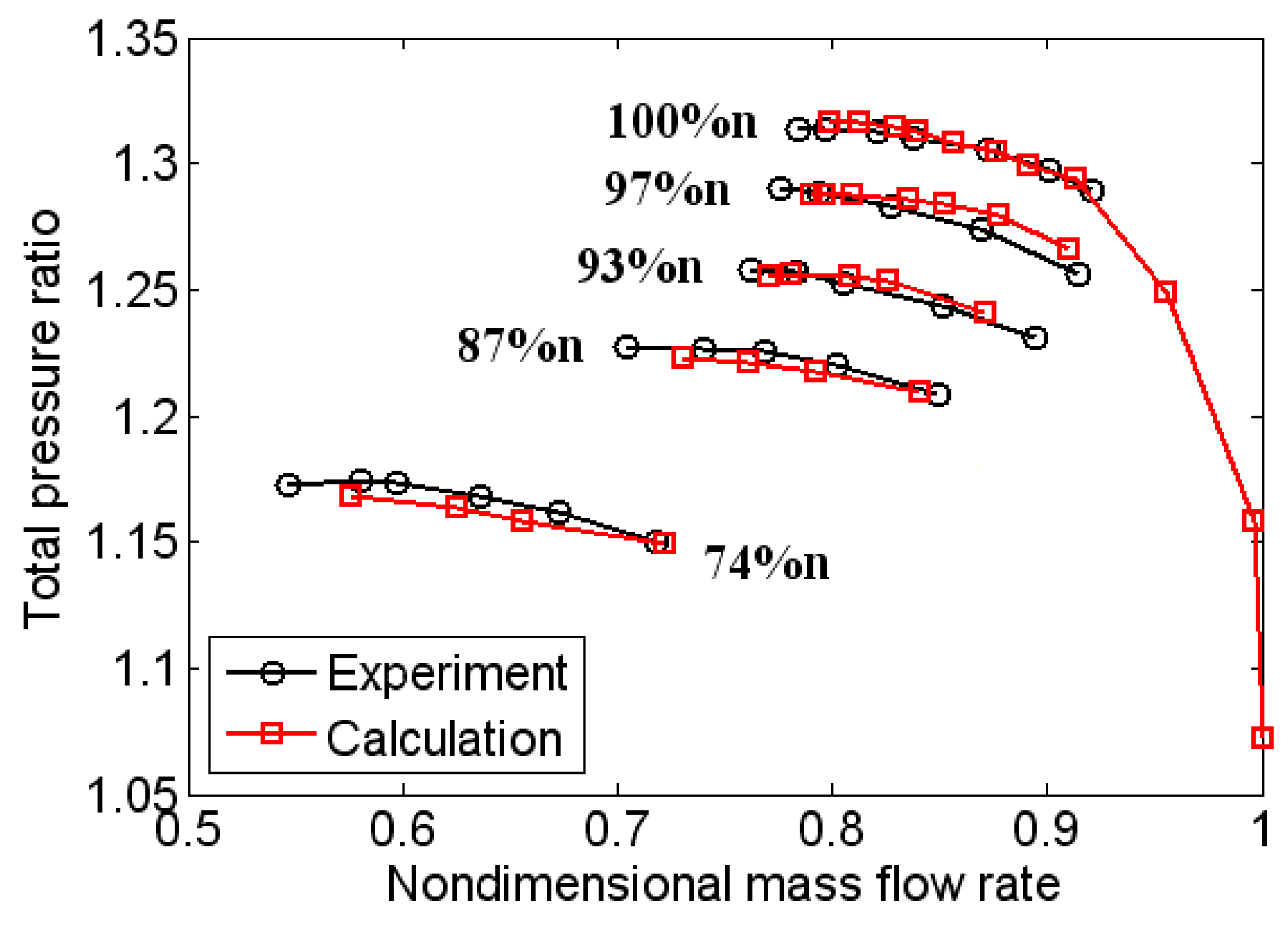
4.1. Aerodynamic Performance

A comparison of the rotor aerodynamic performance at different speeds between the numerical simulations and the experiments is shown in Figure 7. The mass flow-averaged total pressure at the back of the blade trailing edge (1 times the length of chord) was divided by that at front of the blade leading edge (0.5 times the length of chord) to evaluate the total pressure ratio. The numerical curves are basically consistent with the experimental results.

4.2. Modal Analysis of the Rotor Blade

Modal analysis of the blade is carried out to define the excitation force before the fluid-structure simulation. The first and second bending frequencies and the first torsion frequency of the blade in both static and dynamic cases are presented in Table 3. Figure 8 shows the first three mode shapes in the dynamic cases of the blade. Compared with the experimental data, the errors of the calculated static frequency are within 2%.

4.3. Aerodynamic Damping

Both the aerodynamic damping and the non-aerodynamic damping are presented with the vibration of the blade in the flow field, denoted as ξ a and ξ m , respectively. The non-aerodynamic damping is due to numerical and mechanical dissipation, as defined by the Rayleigh damping model. It is presented even when the blade is vibrating in a vacuum, and is calculated using the decay rates extracted from the time history of the blade displacement response in the vacuum. The total damping, denoted as ξ t o t , is calculated using the response of the blade displacement in the flow field. The non-aerodynamic and the total damping of the first two natural modes of the BF_1_2 rotor blade are analyzed using a simulation representing complete fluid-structure interaction. Then, aerodynamic damping is calculated by using the non-aerodynamic and total damping results.

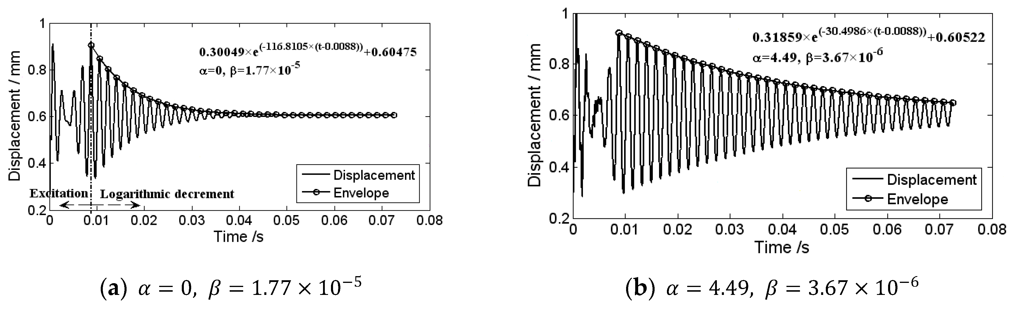
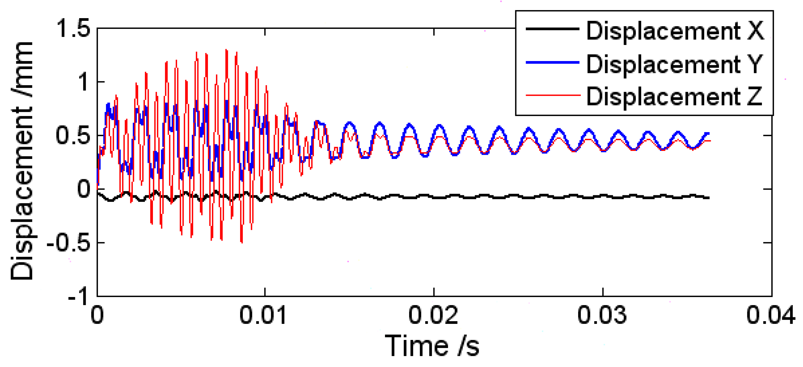
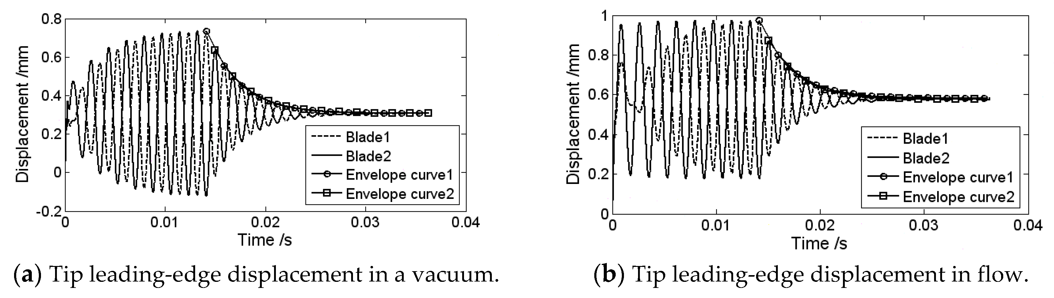
4.3.1. Modal Responses in the Vacuum

The non-aerodynamic damping ξ m is calculated using the decay rates extracted from the time history of the response of the blade displacement in a vacuum. Obviously, this is closely related to the Rayleigh damping constants used to accelerate the convergence of the structure. Figure 9 shows the responses of the tip leading-edge displacement in a vacuum to different Rayleigh damping constants for the first bending modal excitation. The Rayleigh damping constants used in Figure 9a are defined by the frequency range of 0 to the first natural mode, which correspond to the larger β . In Figure 9b, the constants are defined by frequency range of the first natural mode to the third natural mode, which correspond to the smaller β . The amplitude of the excitation force is 0.15 N, which results in noticeable blade tip displacement, but does not plastically deform the blade. The maximum blade displacement due to the bending excitation is small enough (less than 1% of the chord) that the nonlinear aerodynamic effects is negligible.
According to Figure 2, the response envelope for the blade vibrating in a vacuum is A e ( ξ m ω n ( t t 0 ) ) + A , where t 0 and A are the offsets of time and amplitude. In conjunction with Figure 9, the non-aerodynamic damping of ξ m is 0.03167 and 0.00729, which correspond to the Rayleigh damping constants of α = 0 ,   β = 1.77 × 10 5 and α = 4.49 ,   β = 3.67 × 10 6 , respectively.
The blade tip displacement in the vacuum for the second bending modal excitation corresponding to the Rayleigh damping constants of α = 0 and β = 6 × 10 6 is shown in Figure 10. The Rayleigh damping constants are defined by the frequency range of 0 to the second natural mode. Obviously, this is a multi-frequency response; the spectrum analysis is shown Figure 11. The effect of the rotation is taken into account by employing centripetal and Coriolis acceleration terms in the body force. The non-symmetrical nature of the response for the second bending excitation is due to the first bending mode still being present in the response. The response caused by second bending modal excitation is only obtained by filtering the signal. The filtered displacement response for only the second bending modal excitation is shown in Figure 12. The non-aerodynamic damping ξ m achieved by the response envelope is 0.03374.

4.3.2. Modal Response in Flow

Combined with the modal responses in the vacuum that are presented previously, the total damping ξ t o t is calculated using the decay rates extracted from the time history of the blade displacement response in the flow field. The flow field in this section is simulated using a design operation. The response envelope for the blade in flow field is A e ( ξ t o t ω n ( t t 0 ) ) + A . Figure 13 shows the responses of the tip leading-edge displacement in the flow field with respect to different Rayleigh damping constants for the first bending modal excitation; the amplitude of excitation force is 0.15 N. The total damping of ξ t o t is 0.0328 and 0.0857, which correspond to the Rayleigh damping constants α = 0 ,   β = 1.77 × 10 5 and α = 4.49 ,   β = 3.67 × 10 6 , respectively. The total damping values are higher than the corresponding non-aerodynamic damping values, which are shown in Figure 9. This indicates that the blade is aeroelastically stable in the first bending mode of the design operation.
The blade tip displacement and its spectrum analysis in the flow field for the second bending modal excitation, which correspond to the Rayleigh damping constant α = 0 , β = 6 × 10 6 , are shown in Figure 14 and Figure 15, respectively. Obviously, these figures show more significant multi-frequency responses than Figure 10 and Figure 11. Figure 16 shows the filtered displacement response for the second bending modal excitation in the flow field only. The total damping achieved by the response envelope is ξ t o t = 0.0406, which is higher than the corresponding non-aerodynamic damping of ξ m = 0.0337, which is represented in Figure 12. This indicates that the blade is aeroelastic stable in the second bending mode of the design operation.

4.3.3. Aerodynamic Damping Calculation

As previously presented, the non-aerodynamic and total damping values are so small that the influence of the damping on the vibration frequency can be ignored. When f ( t ) is the undamped response of displacement, then the damped response in the vacuum is e ξ m ω k t f ( t ) , where ω k is the natural circle frequency associated with the natural frequency. The vibration damping in flow is composed of two parts, i.e., non-aerodynamic damping and aerodynamic damping. Thus, the damped response in flow can be described by e ( ξ a + ξ m ) ω k t f ( t ) . The total damping in flow can be expressed as ξ t o t = ξ a + ξ m , where ξ t o t and ξ m are predicted quantitatively, as discussed above. Therefore, aerodynamic damping is calculated by the following formula:
ξ a = ξ t o t ξ m .
The total damping only includes the aerodynamic and numerical damping when the Rayleigh damping constants α and β are both zero. Generally, the numerical damping is so small that it can be neglected, and the total damping with the Rayleigh damping constants of α = 0 ,   β = 0 are considered to be mainly due to aerodynamics. Figure 17 shows the aerodynamic damping values which are calculated according to Equation (14) with in accordance with the Rayleigh damping constants α = 0 ,   β = 6 × 10 6 and α = 0 ,   β = 0 for the first bending modal excitation, respectively. As shown in Figure 17, these results basically conform to the predictions. The aerodynamic damping is reduced when the non-dimensional mass flow rate decreases. In particular, the aerodynamic damping value reaches 0 when the non-dimensional mass flow rate is about 0.825, which represents the flutter boundary. This is basically consistent with the experimental results, where the non-dimensional mass flow rate of the flutter boundary is 0.795 [18].
Figure 18 shows the blade tip leading-edge displacement response for zero Rayleigh damping ( α = 0 ,   β = 0 ) at different mass flow rates corresponding to A, B, and C operating conditions, as presented in Figure 17. From A to C, the convergent blade displacement response gradually becomes divergent, indicating that the blade tends to suffer from instability.
Clearly, the ξ m and ξ t o t are affected by mechanical damping. Furthermore, the influence of mechanical damping ( α , β ) on the aerodynamic damping using the fluid-structure interaction simulation is studied. The Rayleigh damping constants are calculated using Equation (10) and Equation (11) from a considered frequency range of f l o to f u p . The aerodynamic damping results with different Rayleigh damping constants, which are calculated using different frequency ranges, are shown in Table 4.
The first three natural frequencies in the dynamic response are f 1 , f 1 , and f 3 . Table 4 shows the significant difference in total damping ξ t o t and non-aerodynamic damping ξ m with various Rayleigh damping, whereas the values of aerodynamic damping ξ a are almost the same except for those defined by the frequency range of 0 to f 1 , which correspond to the largest β . This indicates that the damping constant β is not too large for the accurate prediction of aeroelastic stability. However, the computational cost generally increases as β decreases. The results in Table 4 suggest that the Rayleigh damping constants defined by the frequency range of 0 to the second natural mode are appropriate when considering both computational accuracy and cost for the coupled fluid-structure simulation.
Furthermore, the effect of the amplitude of the excitation force on predicted aerodynamic damping is also studied. Figure 19 shows the amplitudes of the blade vibration in a vacuum and a flow field when the time of excitation is constant. The blade vibration amplitude is defined as the amplitude at the end of excitation. Figure 20 shows the corresponding results of aerodynamic and non-aerodynamic damping.
As shown in Figure 19, for the same excitation force, the vibration amplitudes in the vacuum are all higher than that of the flow due to aerodynamic damping. The amplitude of blade vibration increases approximately linearly alongside increasing excitation force amplitude. As shown in Figure 20, non-aerodynamic damping is almost constant with increasing amplitude of excitation force. However, the aerodynamic damping values show a significant decrease in accordance with the increasing amplitude of excitation force once the amplitude becomes larger than 0.15 N. This phenomenon demonstrates that nonlinear vibration (a large amplitude) has a significant effect on aeroelastic stability. The aerodynamic damping values are all positive, indicating that the blade vibration is stable at the design point. However, the aerodynamic damping transits from positive to negative, indicating that the blade tends to suffer from instability. The aerodynamic damping is almost the same when the amplitude of excitation force is small (0.1–0.15 N), which corresponds to a small vibration amplitude (less than 1% of the chord, as shown in Figure 19), which is considered to be linear. In addition, for the same excitation force, aerodynamic damping values near the flutter points are less than those near the design conditions.
Moreover, IBPA is a key factor for aeroelastic stability in turbomachinery. The applicability of this method for dealing with non-zero IBPAs is illustrated by predicting the aerodynamic damping at an IBPA of 180°, where the double passage model is employed. Figure 21 shows the blade displacement response both in a vacuum and in a flow field. An apparent IBPA of 180° is presented below.
A comparison of aerodynamic damping between an IBPA of 0° and an IBPA of 180° is shown in Figure 22. The blade is more stable at an IBPA of 0° than at an IBPA of 180°.

5. Conclusions

Based on the logarithmic decrement theory, a novel prediction method for aerodynamic damping of a blade under different modes and IBPAs is developed by employing excitation force with different modal frequencies.
This method proves to be suitable when compared with the experiment results using a transonic rotor. A comparison of aerodynamic damping with different Rayleigh damping constants shows that a larger beta damping constant causes inaccurate predictions of the blade aeroelastic stability. It also suggests that Rayleigh damping constants that are defined by the frequency range of zero to the second natural mode are appropriate for this method.
The effect of the amplitude of excitation force on the predicted aerodynamic damping has been investigated. The results show that non-aerodynamic damping is almost the same when the amplitude of excitation force varies, while aerodynamic damping shows the opposite result. This indicates that the nonlinear vibration with a large amplitude has a significant effect on the blade aeroelastic stability.
The applicability of this method for dealing with non-zero IBPAs has also been illustrated. Aerodynamic damping with an IBPA of 180° is predicted by employing the double passage model and different phases of the excitation force. The results show that aerodynamic damping with an IBPA of 180° is higher than when using an IBPA of 0°.

Author Contributions

Conceptualization, J.L. and X.Y.; Data curation, J.L.; Investigation, J.L.; Methodology, J.L.; Supervision, A.H.; Validation, Y.C.; Writing—Original Draft, J.L.; Writing—Review & Editing, A.H., X.Y., Y.C. and M.L.

Funding

This work is supported by the Special Funds of the Foshan Technology Innovation Team of China (No. 2016lt100123).

Conflicts of Interest

The authors declare no conflict of interest.

References

  1. Mikolajczak, A.; Arnoldi, R.A.; Snyder, L.E.; Stargardter, H. Advances in fan and compressor blade flutter analysis and predictions. J. Aircr. 2008, 12, 325–332. [Google Scholar] [CrossRef]
  2. Chen, M.Z. Development of fan/compressor techniques and suggestions on further researches. J. Aerosp. Power 2002, 17, 1–15. (In Chinese) [Google Scholar]
  3. Lane, F. System Mode Shapes in the Flutter of Compressor Blade Rows. J. Aeronaut. Sci. 1956, 23, 54–66. [Google Scholar] [CrossRef]
  4. Carta, F.O. Coupled Blade-Disk-Shroud Flutter Instabilities in Turbojet Engine Rotors. J. Eng. Gas Turbines Power 1967, 89, 419–426. [Google Scholar] [CrossRef]
  5. Bendiksen, O. Aeroelastic problems in turbomachines. In Proceedings of the AIAA/ASME/ASCE/AHS/ASC Structures, Structural Dynamics and Materials Conference, Long Beach, CA, USA, 2–4 April 1990; American Institute of Aeronautics and Astronautics: Washington, DC, USA, 1990; pp. 1736–1761. [Google Scholar]
  6. Cinnella, P.; De Palma, P.; Pascazio, G.; Napolitano, M. A Numerical Method for Turbomachinery Aeroelasticity. J. Turbomach. 2004, 126, 310–316. [Google Scholar] [CrossRef]
  7. Srivastava, R.; Bakhle, M.A.; Keith, T.G.; Hoyniak, D. Aeroelastic analysis of turbomachinery: Part II—Stability computations. Int. J. Numer. Methods Heat Fluid Flow 2004, 14, 382–402. [Google Scholar] [CrossRef]
  8. He, L.; Wang, D.X. Concurrent Blade Aerodynamic-Aero-elastic Design Optimization Using Adjoint Method. J. Turbomach. 2010, 133, 011–021. [Google Scholar] [CrossRef]
  9. Sisto, F.; Thangam, S.; Abdel-Rahim, A. Computational prediction of stall flutter in cascaded airfoils. AIAA J. 1991, 29, 1161–1167. [Google Scholar] [CrossRef]
  10. Hwang, C.J.; Fang, J.M. Flutter Analysis of Cascades Using an Euler/Navier-Stokes Solution-Adaptive Approach. J. Propuls. Power 2008, 15, 54–63. [Google Scholar] [CrossRef]
  11. Sadeghi, M.; Liu, F. Computation of cascade flutter by uncoupled and coupled methods. Int. J. Comput. Fluid Dyn. 2005, 19, 559–569. [Google Scholar] [CrossRef]
  12. Sadeghi, M.; Liu, F. Investigation of Mistuning Effects on Cascade Flutter Using a Coupled Method. J. Propuls. Power 2007, 23, 266–272. [Google Scholar] [CrossRef] [Green Version]
  13. Zheng, Y.; Yang, H. Coupled fluid-structure flutter analysis of a transonic fan. Chin. J. Aeronaut. 2011, 24, 258–264. [Google Scholar] [CrossRef]
  14. Debrabandere, F.; Tartinville, B.; Hirsch, C.; Coussement, G. Fluid–Structure Interaction Using a Modal Approach. J. Turbomach. 2012, 134, 051–057. [Google Scholar] [CrossRef]
  15. Zhang, M.; Hou, A.; Zhou, S.; Yang, X. Analysis on Flutter Characteristics of Transonic Compressor Blade Row by a Fluid-Structure Coupled Method. In Proceedings of the ASME Turbo Expo 2012: Turbine Technical Conference and Exposition, Copenhagen, Denmark, 11–15 June 2012; American Society of Mechanical Engineers: New York, NY, USA, 2013; pp. 1519–1528. [Google Scholar]
  16. Cheng, Z.; Madsen, H.A.; Gao, Z.; Moan, T. Numerical study on aerodynamic damping of floating vertical axis wind turbines. J. Phys. Conf. Ser. 2016, 753, 102001. [Google Scholar] [CrossRef]
  17. Gottfried, D.A.; Fleeter, S. Aerodynamic Damping Predictions in Turbomachines Using a Coupled Fluid-Structure Model. J. Propuls. Power 2005, 21, 327–334. [Google Scholar] [CrossRef]
  18. Song, Z.H.; Feng, Y.C.; Wang, Y.W. The Experimental Research in the Flutter Characteristics of the BF-1 Series of Rotors. In Proceedings of the Fifth International Symposium on Unsteady Aerodynamics and Aeroelasticity of Turbomachines and Propellers, Beijing, China, 18–21 September 1989; pp. 301–311. [Google Scholar]
  19. ANSYS. Inc. ANSYS 17.2 Help Manual [R]; ANSYS: Canonsburg, PA, USA, 2016. [Google Scholar]
  20. Inman, D.J. Engineering Vibration, 4th ed.; Prentice Hall Press: Upper Saddle River, NJ, USA, 2013; pp. 215–220. [Google Scholar]
Figure 1. Fluid-structure interaction algorithm.
Applsci 09 04411 g001
Figure 2. Logarithmic decay of vibration displacement.
Applsci 09 04411 g002
Figure 3. Modal excitation force with different inter-blade phase angles (IBPAs).
Applsci 09 04411 g003
Figure 4. Testing rotor BF_1_2.
Applsci 09 04411 g004
Figure 5. FE model.
Figure 5. FE model.
Applsci 09 04411 g005
Figure 6. Fluid simulation mesh.
Applsci 09 04411 g006
Figure 7. Nondimensionalized rotor aerodynamic performance map.
Applsci 09 04411 g007
Figure 8. Blade mode shape.
Applsci 09 04411 g008
Figure 9. Tip leading-edge displacement in a vacuum for the first modal excitation.
Applsci 09 04411 g009
Figure 10. Tip leading-edge displacement in a vacuum for the second modal excitation.
Applsci 09 04411 g010
Figure 11. Spectrum analysis for the tip leading-edge displacement.
Applsci 09 04411 g011
Figure 12. Tip leading-edge displacement in a vacuum for the second modal excitation after filtering.
Applsci 09 04411 g012
Figure 13. Tip leading-edge displacement in flow for the first modal excitation.
Applsci 09 04411 g013
Figure 14. Tip leading-edge displacement in flow for the second modal excitation.
Applsci 09 04411 g014
Figure 15. Spectrum analysis for tip leading-edge displacement in flow.
Applsci 09 04411 g015
Figure 16. Tip leading-edge displacement in flow for the second modal excitation after filtering.
Applsci 09 04411 g016
Figure 17. Comparison of aerodynamic damping.
Applsci 09 04411 g017
Figure 18. Tip leading-edge displacement in flow for the first modal excitation for α = 0 ,   β = 0 .
Applsci 09 04411 g018
Figure 19. Tip leading-edge vibration amplitude for different excitation force amplitudes.
Applsci 09 04411 g019
Figure 20. ξ a and ξ m for different excitation force amplitudes.
Applsci 09 04411 g020
Figure 21. Tip leading-edge displacement for the first modal excitation at IBPA of 180°.
Applsci 09 04411 g021
Figure 22. Comparison of aerodynamic damping between an IBPA of 0° and an IBPA of 180°.
Applsci 09 04411 g022
Table 1. Main Aerodynamic Parameters.
Mass Flow (kg/s)Ratio of Total PressureRotating Speed (r/min)Blade NumberRelative Mach Number of Blade Tip
12.931.2516,500341.08
Table 2. Blade Material Data.
Density (kg/m3)Young’s Modulus (pa)Poisson’s Ratio
78002.2 × 10110.3
Table 3. Modal Analysis of the Blade.
ModeCalculated Static Frequency (Hz)Experimental Static Frequency (Hz)Calculated Dynamic Frequency (Hz)Error of Static Frequency (%)
1355.8363.0566.31.99
21470.91489.51664.71.25
32112.121492160.21.72
Table 4. Damping of Rotor Blade.
f l o w e r 000 f 1 f 1
f u p p e r f 1 f 2 f 3 f 2 f 3
ξ m 0.03170.01090.00840.00870.0073
ξ t o t 0.03280.01210.00970.01000.0086
ξ a 0.00110.00130.00130.00130.0013

