Article

Chatter Mitigation in Milling Process Using Discrete Time Sliding Mode Control with Type 2-Fuzzy Logic System

by
Satyam Paul
1 and
Ruben Morales-Menendez
2,*
1
School of Science and Technology, Örebro University, 70182 Örebro, Sweden
2
School of Engineering and Sciences, Tecnológico de Monterrey, Monterrey 64849 NL, Mexico
*
Author to whom correspondence should be addressed.
Appl. Sci. 2019, 9(20), 4380; https://doi.org/10.3390/app9204380
Submission received: 2 August 2019 / Revised: 26 September 2019 / Accepted: 11 October 2019 / Published: 16 October 2019
(This article belongs to the Collection Recent Applications of Active and Passive Noise Control)

Abstract

:
In order to achieve a high-quality machining process with superior productivity, it is very important to tackle the phenomenon of chatter in an effective manner. The problems like tool wear and improper surface finish affect the milling process and are caused by self-induced vibration termed as chatter. A strategy to control chatter vibration actively in the milling process is presented. The mathematical modeling of the process is carried out initially. In this paper, an innovative technique of discrete time sliding mode control (DSMC) is blended with the type-2 fuzzy logic system. The proposed active controller results in a significantly high mitigation of vibration. The DSMC is linked to the time-varying gain which is an innovative approach to mitigate chattering. The theorem is laid down which validates that the system states are bounded in the case of DSMC-type-2 fuzzy. Stability analysis is carried out using Lyapunov candidate. The nonlinearities linked with the cutting forces and damper friction are handled effectively by using the type-2 fuzzy logic system. The performance of the DSMC-type-2 fuzzy concept is compared with the discrete time PID (D-PID) and discrete time sliding mode control for validating the effectiveness of the controller. The better performance of DSMC-type-2 fuzzy over D-PID and DSMC-T1 fuzzy in the minimization of milling chatter are validated by a numerical analysis approach.

1. Introduction

Self-generated vibration in the machining process degrades the quality of the finished product and should be given due consideration as it is an important factor associated with manufacturing industries [1]. The self-induced vibration termed as chatter is an important phenomenon which effects the machining process resulting in dimensional inaccuracy and minimization in the removal rate of the material (MRR). The chatter phenomenon also results in low quality finish with significant tool wear [2]. The chatter in the milling process generates a significant amount of vibration which incurs an improper finish due to the change in surface roughness resulting in less production and high delivery time [3].
Machining chatter can be mitigated by utilizing three different techniques. The first option is the utilization of stability lobe diagram (SLD) where the parameters of the machine are choose from outside the stability lobes thus compensating the chattering phenomenon [4]. The second option is to tweak the regenerative effect with the approach of machine parameter change in a continuous manner. The main methodology associated with the second option is spindle speed variation (SSV) [5]. The third option is the alteration of machine tool dynamics for expanding the chatter boundary by implementing active or passive strategies. The most common type of passive devices used for vibration mitigation of the machining process are tuned mass damper (TMD) and dynamic vibration absorber (DVA) [6]. Yang et al. [7] have depicted an innovative concept for the mitigation of chatter in the milling process by making use of TMD. The main positive aspect of passive devices is it is very much flexible with easy instillation, also it is of low cost and does not make the system unstable. However, the main constraint encountered by passive devices is the necessity to tune it accurately at particular frequencies for superior vibration mitigation. So it is not always advantageous to use passive devices due to minimal robustness while handling changing machining conditions. The active control system is a combination of suitable controllers, efficient sensors and dampers which, when implemented, improves the performance of machining with less vibration in the machine tool [8]. The technique of active damper control by implementing the methodology of direct feedback velocity is depicted in the works of Ganguli et al. [9]. The innovative mechanism of active damper for the mitigation of chatter which is justified experimentally has been investigated by Harms et al. [10]. An effective mechanism is proposed in [11] involving an electrostrictive approach in combination with an active damper. The control law was established by using the technique of linear quadratic Gaussian (LQG) which proved to be efficient in terms of robustness and productivity. A concept involving a predictive model for active control of chatter vibration with input constraints is suggested in the work of Zhang et al. [12]. Chen et al. [13] developed an adaptive algorithm on the basis of Fourier series for active control of chatter. Weremczuk et al. [14] proposed an algorithm to control milling chatter using an active approach and harmonic excitation methodology. Alharbi et al. [15] implemented the concept of PID controller for chatter mitigation in the milling process.
Cutting forces associated with the machining process involve nonlinearities [16]. The presence of nonlinearities in a cutting force model is an important aspect and should be analyzed thoroughly [17,18,19]. Exhaustive research unveils that nonlinear modeling is an area of great interest and should be given importance. Moradi et al. [20] demonstrated that the cutting forces are a combination of square as well as cubic polynomial terms which are nonlinear in nature.
In situations where the model of the milling procedure is unknown, fuzzy logic comes in very handy and effective. Fuzzy logic has earned great research reputation due to its capacity to do nonlinear mapping thus maintaining robustness and simplicity. Liang et al. [21] proposed an innovative technique to control chatter in end milling by utilizing the concept of fuzzy logic system. Stability analysis along with uncertainty compensation of the milling process was carried out efficiently by Sims et al. [22]. An effective LMI approach was utilized for the development of static output feedback controller for nonlinear systems described by a continuous-time T-S model [23]. An output PDC (OPDC) controller is proposed and the quadratic Lyapunov technique is implemented to extract the asymptotic stability of the OPDC controller. A type-2 fuzzy logic system performs significantly better than type-1 fuzzy logic system due to its possession of additional DOF which is known as a footprint of uncertainty [24,25]. The concept and methodical approach associated with type-2 fuzzy was demonstrated in the work of Liang and Mendel [26]. The most effective way to handle uncertainities is the implementation of type-2 fuzzy logic because it performs better than type-1 fuzzy logic [27]. Hassani et al. [28] utilized an immeasurable premise variable for detecting the faults in T-S fuzzy systems. In order to tackle the uncertainties in a suitable manner, interval type-2 fuzzy sets were introduced. Moreover, a comparison between robust unknown input fault detection observers (UIFDO) and an existent reference is carried out to validate that the interval type-2 T-S fuzzy model is superior to type-1. In the work of Paul et al. [29], it is demonstrated that the type-2 fuzzy PD/PID controller performed better than the classical fuzzy PD/PID controller in the control of vibration of the structure. An innovative concept involving type-1 and type-2 fuzzy logic systems are proposed for pitch angle controlled wind energy systems as an application for the performance investigation. The results show that the type-2 fuzzy logic system offers better performance in comparison to type-1 fuzzy logic systems [30]. A comparison between type-1 fuzzy and type-2 fuzzy logic controllers implemented in laser tracking systems was carried out by Bai et al. [31]. The simulation results validated that the type-2 fuzzy controller outperformed the type-1 fuzzy controller. The exhaustive research reveals that type-2 fuzzy is superior to type-1 fuzzy. This fact initiate the research motivation of implementing type-2 fuzzy controllers for chatter attenuation. The numerical analysis validated that the results were improved by the incorporation of a type-2 fuzzy logic system.
Sliding mode control (SMC) is a superior control mechanism for vibration attenuation in milling tools since SMC exhibits the same movement pattern as that of the tool vibration pattern. SMC is most suited for nonlinear systems due to its specific design criteria [32]. An SMC controller handles the external noises and fluctuations associated with the parameters with greater effectiveness. Moradi et al. [33] investigated the chatter phenomenon in the turning process and proposed SMC for chatter attenuation. A synergistic combination of proportional-integral (PI) control and fuzzy sliding mode control (FSMC) was proposed by Zhao et al. [34]. In their work, fuzzy logic is utilized to compensate the nonlinearities whereas the PI control is implemented for chatter control. Ma et al. [35] developed an active sliding mode control strategy to mitigate the chatter in the turning process utilizing the concept of dynamic output feedback sliding surface combined with an adaptive law for noise approximation. A model based on an adaptive neuro-fuzzy inference system (ANFIS) and a novel fuzzy sliding mode controller (FSMC) was developed to control the vibration on vehicle the suspension system [36]. An efficient controller based on adaptive hybrid control of interval type-2 fuzzy controller in combination with a new modified sliding mode control is developed to control the vibration in magnetorheological mount [37]. Discrete time sliding mode control (DSMC) is an efficient controller for vibration attenuation due to its criteria of sampling period which is an important aspect in vibration control.
Proportional-integral derivative (PID) control has been widely applied in industrial processes [38,39]. It is an important control strategy because it demonstrates superior capabilities without the knowledge of the model and also due to its simplicity, as well as being incorporated with distinct physical meanings. Alharbi et al. [15] implemented the concept of PID controller for chatter mitigation in the milling process. So in this paper, the PID controller is considered as a potential controller for the comparison with the developed controller.
This work is carried out by implementing the third option “active control of chatter”. In the first instance along x and y components, the mathematical modeling of the milling process is done. Then the nonlinearities are identified for efficient compensation. The actual outcomes of active vibration samper (AVD) was simulated using Matlab/Simulink for chatter suppression. The modeling is accomplished by taking into consideration the dynamics of AVD. Discrete time sliding mode (DSMC) generates the control signals which are used for the suppression of chatter. DSMC is combined with type-2 fuzzy logic (DSMC-T2 fuzzy) for efficiency. The implementation of the type-2 fuzzy system ensures that the nonlinearities are compensated in an effective manner. The approach of Lyapunov stability analysis is implemented to prove that the DSMC-T2 fuzzy controller is a stable one. The chatter attenuation is achieved by the combined action of DSMC-T2 fuzzy with AVD. The wide significance of the concept and methodology is validated using numerical analysis. The results of the DSMC-T2 fuzzy are compared with discrete time sliding mode control with type-1 fuzzy (DSMC-T1 fuzzy) and discrete time PID (D-PID) to prove the effectiveness of the most suited controller. The numerical analysis results validate that the methodology of chatter control can be implemented effectively in the real time milling system. This can be achieved by designing and developing an AVD and placing it on the top of the milling spindle.

2. Modeling of the Milling Process with Active Control

In case of a milling tool with n evenly spaced teeth which is almost flexible to the rigid workpiece, a generalized 2-degrees of freedom mathematical model is [40,41]:
M m x ¨ c ( t ) + C m x ˙ c ( t ) + K m x c ( t ) = F m ( t )
the equivalent mass, damping and stiffness matrices are illustrated by the terms M m , C m and K m , respectively.
M m = m m x 0 0 m m y 2 × 2 , C m = c m x 0 0 c m y 2 × 2 , K m = k m x 0 0 k m y 2 × 2
Again, x c ( t ) = [ x y ] T illustrates the displacement of the tool along x and y components. F m ( t ) = [ F f x F f y ] T illustrates x and y component cutting forces. Along the x and y axes, the new form of Equation (1) is:
m m x 0 0 m m y x ¨ y ¨ + c m x 0 0 c m y x ˙ y ˙ + k m x 0 0 k m y x y = F f x F f y
which generates:
m m x x ¨ + c m x x ˙ + k m x x = F f x m m y y ¨ + c m y y ˙ + k m y y = F f y
It is utter necessary to elaborate the dynamics of the cutting forces along the x and y components. 
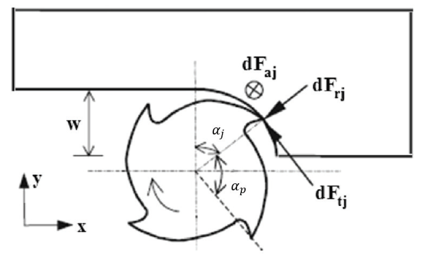
Figure 1 illustrates the dynamics of the milling process [42,43]. The closed form equations representing the nonlinear cutting forces along x and y components are illustrated as [20]:
F x = + N 2 π ζ 1 Δ x 3 + η 1 Δ y 3 + ζ 2 Δ x 2 + η 2 Δ y 2 + ζ 3 Δ x + η 3 Δ y + 3 γ 1 Δ x 2 Δ y + 3 γ 2 Δ x Δ y 2 + 2 γ 3 Δ x Δ y + γ 4 F y = N 2 π ζ 1 * Δ x 3 + η 1 * Δ y 3 + ζ 2 * Δ x 2 + η 2 * Δ y 2 + ζ 3 * Δ x + η 3 * Δ y + 3 γ 1 * Δ x 2 Δ y + 3 γ 2 * Δ x Δ y 2 + 2 γ 3 * Δ x Δ y + γ 4 *
where Δ x + x ( t τ ) = x ( t ) and Δ y + y ( t τ ) = y ( t ) . The time delay is illustrated as τ = 2 π n Ω , Ω = spindle speed ( r a d / s ) . If we consider the present and previous tool period instances, then it is represented by x ( t ) y ( t ) and x ( t τ ) y ( t τ ) , respectively. Considering the start immersion angle as 0 and the exit angle as π 2 , The calculation of the coefficients for half-immersion up-milling is:
ζ 1 = 1 4 ξ 1 + 3 4 π δ 1 , η 1 = 1 4 δ 1 + 3 4 π ξ 1 , ζ 2 = 1 3 ξ 2 + 2 δ 2 , η 2 = 1 3 δ 2 + 2 ξ 2 , ζ 3 = 1 2 ξ 3 + 1 2 π δ 3 , η 3 = 1 2 δ 3 + 1 2 π ξ 3 , γ 1 = 1 4 δ 1 + 1 4 π ξ 1 , γ 2 = 1 4 ξ 1 + 1 4 π δ 1 , γ 3 = 1 3 δ 2 + ξ 2 , γ 4 = ξ 4 + δ 4 ζ 1 * = 1 4 δ 1 + 3 4 π ξ 1 , η 1 * = 1 4 ξ 1 3 4 π δ 1 , ζ 2 * = , 1 3 δ 2 + 2 ξ 2 , η 2 * = 1 3 ξ 2 2 δ 2 , ζ 3 * = 1 2 δ 3 + 1 2 π ξ 3 , η 3 * = 1 2 ξ 3 1 2 π δ 3 , γ 1 * = 1 4 ξ 1 1 4 π δ 1 , γ 2 * = 1 4 δ 1 + 1 4 π ξ 1 , γ 3 * = 1 3 ξ 2 δ 2 , γ 4 * = δ 4 + ξ 4
where 0 is the start immersion angle and π 2 is the exit angle. Moreover, ξ 1 , ξ 2 , ξ 3 , ξ 4 , δ 1 , δ 2 , δ 3 , δ 4 are the cutting force coefficients.

Active Vibration Damper (AVD) for Active Control Mechanism
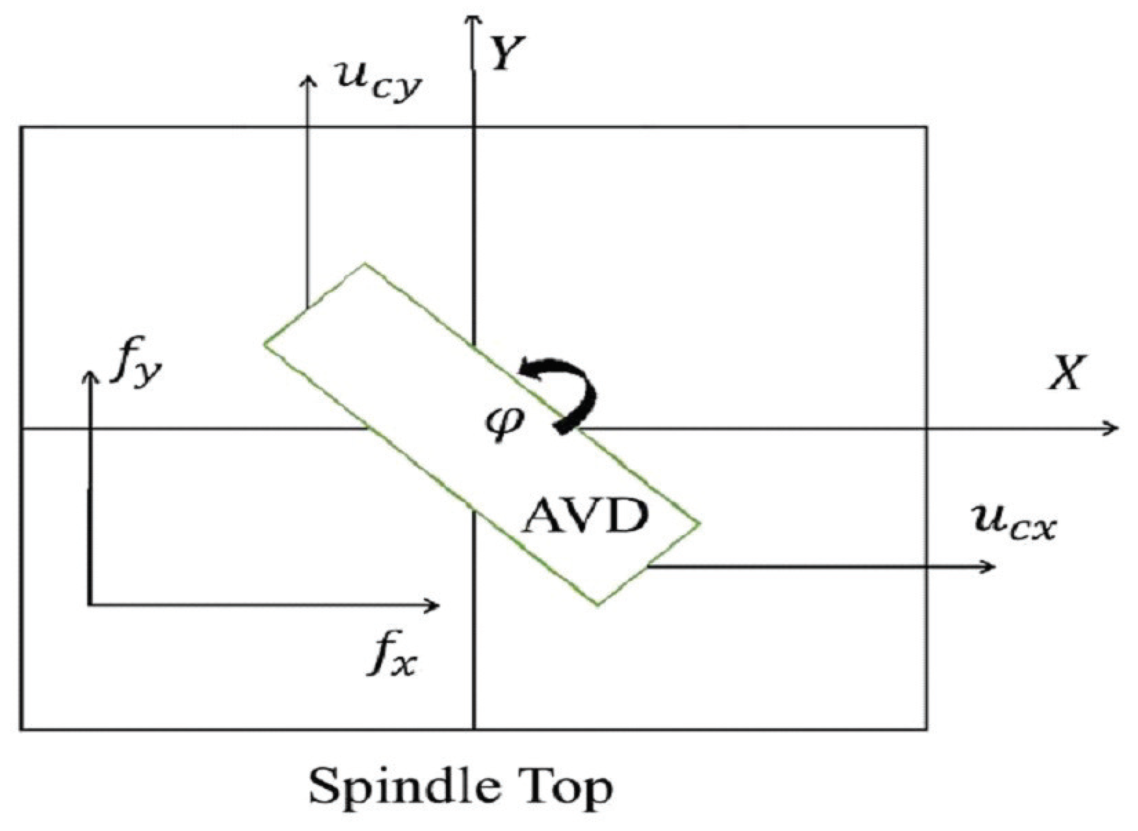
As seen from Figure 2, AVD is placed on the top of the spindle to minimize the tool chattering generated by the external force. The main mechanism behind AVD is that it works as a linear servo actuator. A linear actuator converts the rotary motion of the motor to the required linear motion. The position of the AVD is at the center of mass (CM) and it makes an inclination φ with CM. It is considered to be an effective placement due to the mitigation of spacing problem of the AVD. The efficient placement of damper is cost effective, thus mitigating the requirement of two dampers. The combination of the modeling equation and control force u c yields:
M m x ¨ c ( t ) + C m x ˙ c ( t ) + K m x c ( t ) = F m ( t ) + u c d c
the control signals impinged on the damper along both axes and is illustrated by u c = u c x , u c y T 2 × 1 ; d c = d c x , d c y 2 × 1 is the combined damping-fricton effect resolved along two axes. Now with the control signals the closed loop Equation (1) can be illustrated as:
m m x x ¨ + c m x x ˙ + k m x x = F f x + u c x d c x m m y y ¨ + c m y y ˙ + k m y y = F f y + u c y d c y
The damper force f d is:
f d = m d ( g ¨ i + γ ¨ i )
where m d = mass of the damper, g ¨ i = acceleration of the damper, γ ¨ i = tool acceleration. Moreover, γ ¨ i 2 = a i , x + a i , y implies the relative accelerations of the tool associated with both the axes. Now, f d can be resolved along the x and y components as follows:
f d = m d ( g ¨ i cos φ + a i , x ) cos φ or f d = m d ( g ¨ i sin φ + a i , y ) sin φ γ ¨ i = a i , x cos φ = a i , y sin φ x ¨ i , x a i , x = g ¨ i cos φ , x ¨ i , y a i , y = g ¨ i sin φ
where φ , x ¨ i , x and x ¨ i , y represent the angle of the damper, relative acceleration of the damper along the x component and the relative acceleration of the damper along y component, respectively. Now, f d is represented mathematically:
f d = m d cos φ cos φ g ¨ i + a i , x = m d sin φ sin φ g ¨ i + a i , y
The control action along the x and y directions represented by u c = u c x u c y T is given by:
u c = m d i x ¨ i , x m d i x ¨ i , y T
It is very important to consider the damper friction, which can be resolved as:
d c x = Λ x ˙ i , x + Γ m d g tanh Υ x ˙ i , x d c y = Λ x ˙ i , y + Γ m d g tanh Υ x ˙ i , y
where Λ , Υ and Γ are termed as damping coefficients associated with the Coulomb friction [44], Moreover, d c = [ d c x d c y ] T . Taking into consideration Equations (8) and (13), the combination of the control methodology with the closed loop system is given by:
m m x x ¨ + c m x x ˙ + k m x x = F f x + u c x Λ x ˙ i , x Γ m d g tanh Υ x ˙ i , x m m y y ¨ + c m y y ˙ + k m y y = F f y + u c y Λ x ˙ i , y Γ m d g tanh Υ x ˙ i , y
In Equation (14), the nonlinear terms are Λ x ˙ i , x + Γ m d g tanh Υ x ˙ i , x , Λ x ˙ i , y + Γ m d g tanh Υ x ˙ i , y , F f x and F f y . The intelligent technique is incorporated to deal with the involved nonlinearities.

3. Discrete Time Sliding Mode Control with Type-2 Fuzzy Compensation

Generally the overall stiffness of machine tools is computed using the static loading test. The stiffness calculated by the static test, however, in general cases shows hysterics characteristics. This is due to the fact that the contact area of the bearing changes as the load direction changes [45,46]. The stiffness has been modeled considering it to be a nonlinear in nature and is demonstrated effectively in [14]. The hysteric behavior can be handled effectively using the Bouc-Wen model. The behavior of the structure can be modeled using Bouc-Wen method which separates Equation (15) into two parts (elastic and inelastic) as [47]:
f ρ , i = ϵ ρ i k ρ i x ρ i + ( 1 ϵ ρ i ) k ρ i ϕ ρ i
representing the positive numbers by ρ . The function illustrating nonlinearties ( ϕ ρ i ) is:
ϕ ρ i = 1 η ρ i λ ρ i x ˙ ρ i a ρ i η l i 1 a ρ i v ρ i γ ρ i x ˙ ρ i a ρ i η l i 1 v ρ i a ρ i s i g n ( x ˙ ρ i a ρ i ) ] κ x ˙ ρ i
In the above equation, the positive numbers are κ , λ ρ i , γ ρ i , α ρ i , n and η . Moreover, η ρ i and v ρ i represent the stiffness degradation control factor and strength degradation control factor, respectively. The term, E ρ i = ( 1 α ρ i ) 0 t x ˙ ρ i a ρ i Δ ρ i Δ ρ i d t is defined as dissipated hysteretic energy in normal conditions. Moreover, Δ ρ i = ( λ ρ i + γ ρ i ) 1 η ρ i . The stiffness f k n will be considered as nonlinear. The continuous time model of the milling process, which is a closed loop system from Equation (14), is illustrated as:
M m x ¨ c ( t ) + C m x ˙ c ( t ) + f k n ( x ) = F m ( t ) + u c ( t ) d c
It is very important to discretize the milling process model for digitalization and to make it appropriate for the design of computer based control. For this, the following steps are implemented: V 1 t = x c and V 2 t = x ˙ c . The model represented by Equation (17) is illustrated as a state space model by:
Z ˙ ( t ) = A Z + B u + F k n + f n
Again, V ( t ) = V 1 ( t ) V 2 ( t ) , A D = 0 0 0 M m 1 C m , B D = 0 M m 1 , F k n = M m 1 f k n , f n = M m 1 [ F m + d c ]
In the linear system V ˙ = A D V + u c B D , F k n and f n are considered to be the uncertainties. When there is no external excitations, the tool will be at the stable position. So it is justifiable to consider that F k n is bounded, | | F k n | | d s t . The cutting forces and friction forces are bounded, | | f n ( t ) | | d n . The continuous time model is discretized by assuming that the control force and the external forces are constant during the sampling period T. Now considering the relation k T t ( k + 1 ) T to be valid:
f n ( t ) = f n ( k T ) and u c ( t ) = u c ( k T )
considering V ( k ) to be a state vector with A d i s as a state matrix; moreover, A d i s = e A D T and B d i s = input vector, B d i s = e A D τ d τ B D , u c ( k ) = scalar input, F k n ( Z ( k ) ) = model uncertainty matrix and f d n ( k ) = nonlinearity involved in cutting forces and frictional forces; using Equation (18), the discretized model is [48,49]:
V ( k + 1 ) = A d i s Z ( k ) + B d i s u c ( k ) + F k n ( Z ( k ) ) + f d n ( k )
From Equation (20), the discrete time model is:
V ( k + 1 ) = A d i s V ( k ) + B d i s u c ( k ) + F k n ( Z ( k ) ) + f d n ( k )
From the viewpoint of preciseness and for the introduction fuzzy system to compensate nonlinearities, the following step is considered:
V ( k + 1 ) = j z ( k ) + h z ( k ) u c ( k )
where j z ( k ) = A d i s V ( k ) + F k n ( Z ( k ) ) + f d n ( k ) and h z ( k ) = B d i s , A d i s and B d i s are unknown and F k n ( Z ( k ) ) + f d n ( k ) is nonlinear. So the terms j z ( k ) and h z ( k ) will be modeled using the type-2 fuzzy logic technique.
The type-2 fuzzy sets have a greater capability of modeling big magnitude uncertainties with minimal fuzzy rules when compared to the type-1 fuzzy sets. The concept of membership functions in type-2 fuzzy systems is that it is no longer a crisp value and is considered to be in the interval of 0 , 1 [26]. The fuzzy rules are defined as follows:
R i : IF x i is A 1 i and y i is A 2 i and x ˙ i is A 3 i and y ˙ i is A 4 i THEN f z ( k ) is B 1 i R i : IF x i is A 1 i and y i is A 2 i and x ˙ i is A 3 i and y ˙ i is A 4 i THEN g z ( k ) is B 2 i
where the type-2 fuzzy sets are represented by the terms A 1 i , A 4 i , B 1 i , B 2 i . If G A is the membership function, then the type-2 fuzzy set A is expressed as:
A = { ( x , ς ) , G A ( x , ς ) x ϵ R , ς ϵ M x [ 0 , 1 ] }
with ς as an auxiliary variable and M x as a primary membership function validating the relation 0 G A ( x , ς ) 1 . The type-2 fuzzy logic system with jth output can be expressed as:
f u z j = y r j + y l j 2 = 1 2 ( ϕ r j T ( z ) w r j ( z ( k ) ) + ϕ l j T ( z ) w l j ( z ( k ) )
where y l j = i = 1 p f l j i y l j + i = 1 p f r j i y l k i = 1 q f r i + i = 1 q f l i , y r j = i = 1 p f l j i y r j + i = 1 p f r j i y r k i = 1 q f r i + i = 1 q f l i , q l j i = f l i i = 1 q f r i + i = 1 q f l i , and q r j i = f r i i = 1 q f r i + i = 1 q f l i . Again, f l i and f r i are the firing strengths associated with y l j i and y r j i of the i-th rule. So the compensation technique for j z ( k ) and h z ( k ) are applied as follows:
j ^ = 1 2 w r f ( k ) ϕ r f T [ z ( k ) ] + 1 2 w l f ( k ) ϕ l f T [ z ( k ) ] h ^ = 1 2 w r g ( k ) ϕ r g T [ z ( k ) ] + 1 2 w l g ( k ) ϕ l g T [ z ( k ) ]
For Equation (26), the following learning laws are implemented:
w r f ( k + 1 ) w r f ( k ) = Ω 1 ( k ) e m ( k ) ϕ r f T [ z ( k ) ] w l f ( k + 1 ) w l f ( k ) = Ω 2 ( k ) e m ( k ) ϕ l f T [ z ( k ) ] w r g ( k + 1 ) w r g ( k ) = Ω 1 ( k ) u c ( k ) e m ( k ) ϕ r g T [ z ( k ) ] w lg ( k + 1 ) w lg ( k ) = Ω 2 ( k ) u c ( k ) e m ( k ) ϕ lg T [ z ( k ) ]
Again, Ω 1 k and Ω 2 k satisfy the following:
Ω 1 k = Ω 1 k 1 + Φ 1 ( k ) if e m ( k + 1 ) > 1 β 1 e m ( k ) 0 if e m ( k + 1 ) < 1 β 1 e m ( k ) Ω 2 k = Ω 2 k 1 + Φ 2 ( k ) if e m ( k + 1 ) > 1 β 2 e m ( k ) 0 if e m ( k + 1 ) < 1 β 2 e m ( k )
where 0 < Ω 1 ( k ) 1 and 0 < Ω 2 ( k ) 1 . Moreover, the dead-zone parameters are illustrated by β 1 and β 2 . Again,
Φ 1 ( k ) = ϕ r f T [ z ( k ) ] 2 + ϕ r g T [ z ( k ) ] u c ( k ) 2 Φ 2 ( k ) = ϕ l f T [ z ( k ) ] 2 + ϕ l g T [ z ( k ) ] u c ( k ) 2
Now the modeling error e m ( k ) is represented as:
e m ( k ) = v ^ ( k ) v ( k )
where the state of the fuzzy model is represented by v ^ ( k ) ; therefore:
( β 1 + β 2 ) v ^ ( k + 1 ) = j ^ z ( k ) + h ^ z ( k ) u c ( k )
where β 1 and β 2 are positive constant and β 1 , β 2 > 1 , which is a design parameter. For stability analysis, Equation (31) is illustrated as:
( β 1 + β 2 ) v ( k + 1 ) = 1 2 ω r f * ( k ) ϕ r f T [ z ( k ) ] + 1 2 ω l f * ( k ) ϕ l f T [ z ( k ) ] + 1 2 ω r g * ( k ) ϕ r g T [ z ( k ) ] u c ( k ) + 1 2 ω l g * ( k ) ϕ l g T [ z ( k ) ] u c ( k ) + ( ϵ r f + ϵ l f ) + ( ϵ r g + ϵ l g ) u ( k )
where the unknown optimal weights are ω r f * ( k ) , ω l f * ( k ) , ω r g * ( k ) and ω l g * ( k ) . Moreover, ϵ r f , ϵ l f , ϵ r g and ϵ l f are approximation errors which satisfy the relations f = 1 2 ω r f * ( k ) ϕ r f T [ z ( k ) ] + 1 2 ω l f * ( k ) ϕ l f T [ z ( k ) ] + ( ϵ r f + ϵ l f ) , g = 1 2 ω r g * ( k ) ϕ r g T [ z ( k ) ] + 1 2 ω l g * ( k ) ϕ l g T [ z ( k ) ] + ( ϵ r g + ϵ l f ) . Using Equations (31) and (32), the error dynamics can be stated as:
( β 1 + β 2 ) e m ( k + 1 ) = 1 2 w ˜ r f ( k ) ϕ r f T [ z ( k ) ] + 1 2 w ˜ l f ( k ) ϕ l f T [ z ( k ) ] + 1 2 w ˜ r g ( k ) ϕ r g T [ z ( k ) ] u c ( k ) + 1 2 w ˜ l g ( k ) ϕ l g T [ z ( k ) ] u c ( k ) + ξ f + ξ g u c ( k )
satisfying the relations
ω ˜ r f ( k ) = ω r f ( k ) ω r f * ( k ) ω ˜ l f ( k ) = ω l f ( k ) ω l f * ( k ) ω ˜ r g ( k ) = ω r g ( k ) ω r g * ( k ) ω ˜ l g ( k ) = ω l g ( k ) ω l g * ( k )
where ξ f = ϵ r f + ϵ l f + r f and ξ g = ϵ r g + ϵ l g + r g . Moreover, the remainders of the Taylor formula for j ^ and h ^ are illustrated by r f and r g , respectively.
In case of active vibration control, it considered that v d ( k ) = 0 . The equation validating the control error is:
e c k = v d ( k ) v ( k ) = v ( k )
The SMC can be illustrated as:
u c ( k ) = 2 [ K T e c ( k ) 1 2 ( ω r f ( k ) ϕ r f T [ z ( k ) ] + ω l f ( k ) ϕ l f T [ z ( k ) ] ) σ s i g n s ( k ) ] [ ω r g ( k ) ϕ r g T [ z ( k ) ] + ω l g ( k ) ϕ l g T [ z ( k ) ] ]
where e c ( k ) = e c ( k + 1 n ) e c ( k ) T , The vector representing feedback gain is K G = k n k 1 T R n . The sliding mode gain and switching function are represented by σ and s ( k ) , respectively, where the switching function is:
s ( k ) = K G T e c ( k 1 ) + 1 K G T e c ( k )
Since e c ( k + 1 ) + K G T e c ( k ) = s ( k + 1 ) , so:
e c ( k + 1 ) = A D e c ( k ) + B D s ( k + 1 )
where A D = 0 1 0 0 0 0 1 0 0 0 1 k n k 1 R n × n , B D = 0 , 0 , 1 T R n x 1 . Now using the concept from [50], the relation det s I α A D = α n k n + α n 1 k n 1 s + + α k 1 s n 1 + s n is validated. The selection of gains are carried out in the manner of K G = k 1 k n T so that the polynomial λ n + 2 k 1 λ n 1 + + 2 n 2 k n is stable. This signifies that A D is stable. If A D is stable then the Lyapunov equation 2 A D T P A D = Z U has positive definite solutions for Z ; moreover, U = U T > 0 . Using Equations (22), (31) and (32), it can be validated that the modeling error satisfies:
( β 1 + β 2 ) e m ( k + 1 ) = 1 2 ω ˜ r f ( k ) ϕ r f T [ z ( k ) ] + ω ˜ l f ( k ) ϕ l f T [ z ( k ) ] + 2 ξ f + 1 2 ω ˜ r g ( k ) ϕ r g T [ z ( k ) ] + ω ˜ l g ( k ) ϕ l g T [ z ( k ) ] + 2 ξ g u c ( k )
Combining SMC Equation (36) and the equation of the plant, Equation (22), the system equation in closed-loop form is given by:
v ( k + 1 ) = 1 2 ω ˜ r f ( k ) ϕ r f T [ z ( k ) ] + ω ˜ l f ( k ) ϕ l f T [ z ( k ) ] + 2 ξ f + K T e c ( k ) σ s i g n s ( k ) 1 2 ω ˜ r g ( k ) ϕ r g T [ z ( k ) ] + ω ˜ l g ( k ) ϕ l g T [ z ( k ) ] + 2 ξ g u c ( k )
Using Equation (36) and the relation s ( k + 1 ) = K T e c ( k ) v ( k + 1 ) , the following equation can be validated:
e c ( k + 1 ) + K T e c ( k ) + σ s i g n s ( k ) = 1 2 ω ˜ r f ( k ) ϕ r f T [ z ( k ) ] + ω ˜ l f ( k ) ϕ l f T [ z ( k ) ] + 2 ξ f + 1 2 ω ˜ r g ( k ) ϕ r g T [ z ( k ) ] + ω ˜ l g ( k ) ϕ l g T [ z ( k ) ] + 2 ξ g u c ( k )
Now, using Equation (39),
s ( k + 1 ) + σ s i g n s ( k ) = ( β 1 + β 2 ) e m ( k + 1 )
Since s i g n s ( k ) 1 and e m ( k + 1 ) G
1 G s ( k + 1 ) σ G + ( β 1 + β 2 )
where G is the upper bound of the modeling error. The fuzzy model Equation (31) design parameters are illustrated using β 1 and β 2 .
Theorem 1.
If the fuzzy model Equation (31) is implemented for the compensation of the the nonlinear system outlined in Equation (22) with the updated laws:
w r f ( k + 1 ) w r f ( k ) = Ω 1 ( k ) e m ( k ) ϕ r f T [ z ( k ) ] w l f ( k + 1 ) w l f ( k ) = Ω 2 ( k ) e m ( k ) ϕ l f T [ z ( k ) ] w r g ( k + 1 ) w r g ( k ) = Ω 1 ( k ) u c ( k ) e m ( k ) ϕ r g T [ z ( k ) ] w lg ( k + 1 ) w lg ( k ) = Ω 2 ( k ) u c ( k ) e m ( k ) ϕ lg T [ z ( k ) ]
then the uniform stability of the closed loop system is assured and bounded provided that the identification error e m ( k ) is within the range:
e m ( k ) 2 2 ψ ( k ) ξ ¯ Φ 1 ( k ) + Φ 2 ( k )
and the control error satisfies:
e c ( k ) U 2 σ 2 Z 1 + ( β 1 + β 2 ) G σ
with the gain σ of the discrete-time sliding mode controller Equation (36) establishing
σ G K G ( β 1 + β 2 )
Proof of Theorem 1.
The Lyapunov candidate function L ( k ) is selected as:
L ( k ) = 1 2 ω ˜ r f ( k ) 2 + 1 2 ω ˜ l f ( k ) 2 + 1 2 ω ˜ r g ( k ) 2 + 1 2 ω ˜ lg ( k ) 2 + 1 σ 2 e c T ( k ) Z e c ( k )
Now for simplicity, L ( k ) = L 1 ( k ) + L 2 ( k ) ; therefore:
L 1 ( k ) = 1 2 ω ˜ r f ( k ) 2 + 1 2 ω ˜ l f ( k ) 2 + 1 2 ω ˜ r g ( k ) 2 + 1 2 ω ˜ lg ( k ) 2 L 1 ( k ) = 1 2 t r ω ˜ r f T ( k ) ω ˜ r f ( k ) + 1 2 t r ω ˜ l f T ( k ) ω ˜ l f ( k ) + 1 2 t r ω ˜ r g T ( k ) ω ˜ r g ( k ) + 1 2 t r ω ˜ lg T ( k ) ω ˜ lg ( k )
Now Δ L 1 ( k ) = L 1 ( k + 1 ) L 1 ( k ) ,
Δ L 1 ( k ) = 1 2 [ ω ˜ r f ( k + 1 ) 2 ω ˜ r f ( k ) 2 ] + 1 2 [ ω ˜ l f ( k + 1 ) 2 ω ˜ l f ( k ) 2 ] + 1 2 [ ω ˜ r g ( k + 1 ) 2 ω ˜ r g ( k ) 2 ] + 1 2 [ ω ˜ lg ( k + 1 ) 2 ω ˜ lg ( k ) 2 ]
From the updated Equation (27),
Δ L 1 ( k ) = 1 2 [ ω r f ( k ) Ω 1 ( k ) e i ( k ) ϕ r f T [ z ( k ) ] 2 ω ˜ r f ( k ) 2 ] + 1 2 [ ω l f ( k ) Ω 2 ( k ) e i ( k ) ϕ l f T [ z ( k ) ] 2 ω ˜ l f ( k ) 2 ] + 1 2 [ ω r g ( k ) Ω 1 ( k ) u ( k ) e i ( k ) ϕ r g T [ z ( k ) ] 2 ω ˜ r g ( k ) 2 ] + 1 2 [ ω lg ( k ) Ω 2 ( k ) u ( k ) e i ( k ) ϕ lg T [ z ( k ) ] 2 ω ˜ lg ( k ) 2 ] = 1 2 Ω 1 2 ( k ) e m ( k ) 2 [ ϕ r f T [ z ( k ) ] 2 Ω 1 ( k ) e m ( k ) [ ω ˜ r f ( k ) ϕ r f T [ z ( k ) ] + 1 2 Ω 2 2 ( k ) e m ( k ) 2 [ ϕ l f T [ z ( k ) ] 2 Ω 2 ( k ) e m ( k ) [ ω ˜ l f ( k ) ϕ l f T [ z ( k ) ] + 1 2 Ω 1 2 ( k ) e m ( k ) 2 [ ϕ r g T [ z ( k ) ] u ( k ) 2 Ω 1 ( k ) e m ( k ) [ ω ˜ r g ( k ) ϕ r g T [ z ( k ) ] u c ( k ) + 1 2 Ω 2 2 ( k ) e m ( k ) 2 [ ϕ l g T [ z ( k ) ] u ( k ) 2 Ω 2 ( k ) e m ( k ) [ ω ˜ l g ( k ) ϕ l g T [ z ( k ) ] u c ( k )
Implementing the error dynamics of Equation (33) and using Ω 1 ( k ) = Ω 2 ( k ) = ψ ( k ) :
Δ L 1 ( k ) = 1 2 ψ 2 ( k ) e m ( k ) 2 [ ϕ r f T [ z ( k ) ] 2 + ϕ r g T [ z ( k ) ] u c ( k ) 2 ] + 1 2 ψ 2 ( k ) e m ( k ) 2 [ ϕ l f T [ z ( k ) ] 2 + ϕ l g T [ z ( k ) ] u c ( k ) 2 ] 2 ψ ( k ) e m T ( k ) [ ( β 1 + β 2 ) e m ( k + 1 ) ξ f ξ g u c ( k ) ] Δ L 1 ( k ) = 1 2 ψ 2 ( k ) e m ( k ) 2 [ ϕ r f T [ z ( k ) ] 2 + ϕ r g T [ z ( k ) ] u c ( k ) 2 ] + 1 2 ψ 2 ( k ) e m ( k ) 2 [ ϕ l f T [ z ( k ) ] 2 + ϕ l g T [ z ( k ) ] u c ( k ) 2 ] 2 ψ ( k ) e m ( k ) ( β 1 + β 2 ) e m ( k + 1 ) + 2 ψ ( k ) e m ( k ) [ ξ f + ξ g u c ( k ) ]
using Equations (28) and (29) and utilizing the relations ( β 1 + β 2 ) e m ( k + 1 ) > e m ( k ) and ξ ( k ) = ξ f + ξ g u c ( k ) , it is validated that:
Δ L 1 ( k ) 2 ψ ( k ) e m ( k ) 2 + 1 2 ψ 2 ( k ) e m ( k ) 2 ( Φ 1 ( k ) + Φ 2 ( k ) ) + 2 ψ ( k ) e m ( k ) ξ ( k ) ψ ( k ) e m ( k ) 2 + 1 2 ψ 2 ( k ) e m ( k ) 2 ( Φ 1 ( k ) + Φ 2 ( k ) ) + ψ ( k ) ξ ( k ) 2 ψ ( k ) { 1 ψ ( k ) 2 ( Φ 1 ( k ) + Φ 2 ( k ) } e m ( k ) 2 + ψ ( k ) ξ ( k ) 2
Now the boundary condition of the modeling error ξ ( k ) can be validated using:
ξ ( k ) 2 ξ ¯
Now for achieving Δ L 1 ( k ) 0 ,
ψ ( k ) 2 ( Φ 1 ( k ) + Φ 2 ( k ) } e m ( k ) 2 ψ ( k ) ξ ¯ e m ( k ) 2 2 ψ ( k ) ξ ¯ Φ 1 ( k ) + Φ 2 ( k )
If the β selected is too big then the dead zone becomes small. Hence it is concluded that L 1 ( k ) is bounded, which implies that the identification error e m ( k ) is bounded. Again:
L 2 ( k ) = 1 σ 2 e c T ( k ) Z e c ( k )
Now utilizing Equation (38):
Δ L 2 ( k ) = 1 σ 2 e c T ( k ) Z e c ( k ) + 1 σ 2 e c T ( k + 1 ) Z e c ( k + 1 ) = 1 σ 2 e c T ( k ) A D T Z A D Z e c ( k ) + 2 σ 2 e c T ( k ) A D T Z B D s ( k + 1 ) + 1 σ 2 B D T Z B D s 2 ( k + 1 )
Considering the gain as K G 1 = 1 , k 1 k n T and using Equation (37):
s ( k + 1 ) = K G 1 T e c ( k + 1 )
Again, 1 ( β 1 + β 2 ) s ( k + 1 ) + σ s i g n s ( k ) = e m ( k + 1 ) . Moreover, A D = B D = 1 ; then, utilizing Equation (43):
Δ L 2 ( k ) 1 σ 2 e c ( k ) U 2 2 σ K G 1 ( β 1 + β 2 ) G σ 2 Z e c ( k ) + Z 1 + ( β 1 + β 2 ) G σ 2
From Equation (47):
Δ L 2 ( k ) 1 σ 2 e c ( k ) U 2 + Z 1 + ( β 1 + β 2 ) G σ 2
Now Δ L 2 ( k ) is bounded if 1 σ 2 e c ( k ) U 2 Z 1 + ( β 1 + β 2 ) G σ . Therefore, from the works of [51], it can be establish that since L 2 ( k ) is bounded, e c ( k ) is bounded. Since both L 1 ( k ) and L 2 ( k ) are bounded, L ( k ) is bounded. So it implies that the control error e c ( k ) is bounded. □

4. Validation and Results

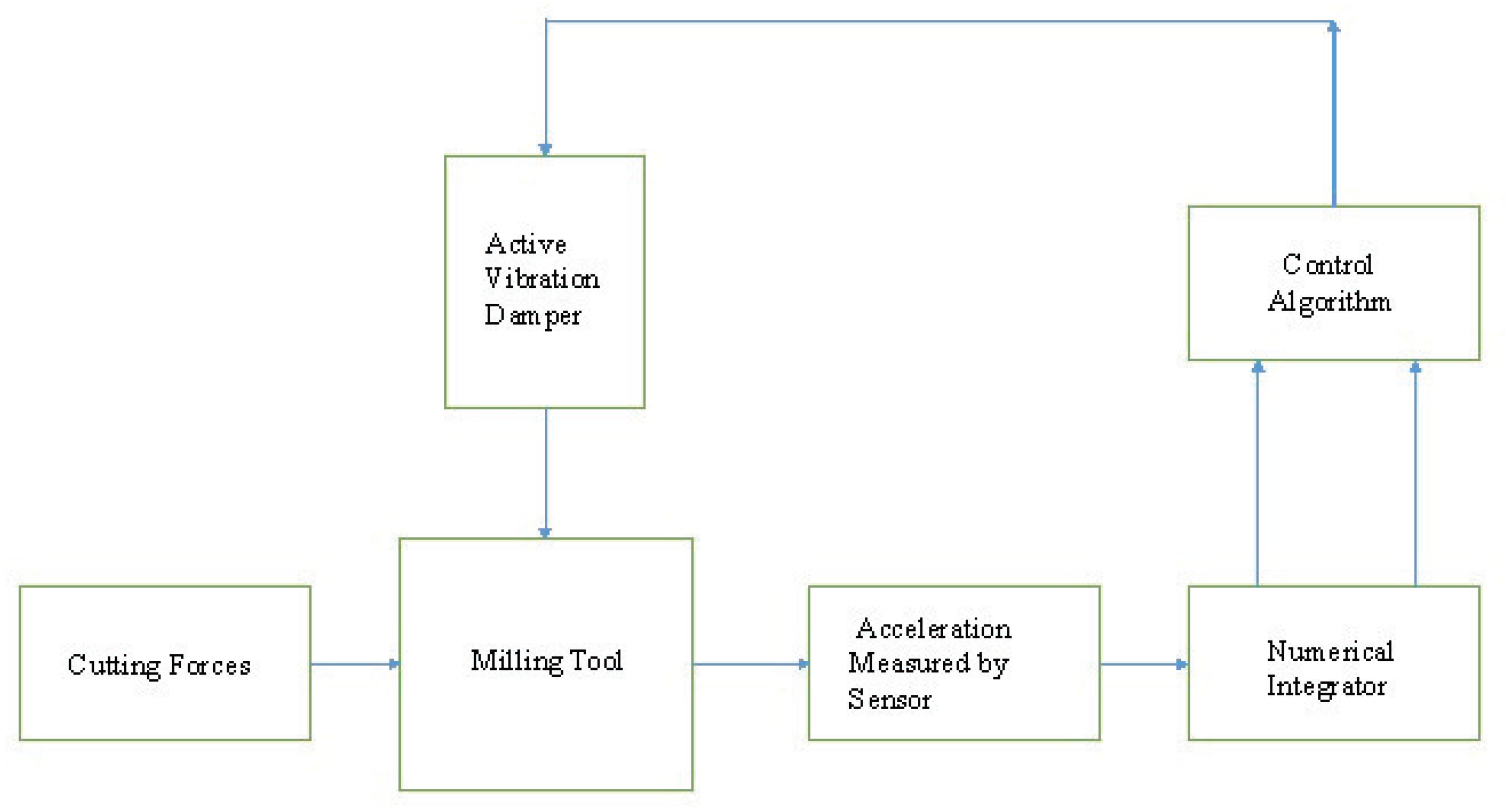
The total control scheme that is essential for having a brief overview of the control process is shown in Figure 3. Initially, to simulate the cutting forces, the cutting conditions are essential. This cutting force has influence on the tool vibration. In the first instance, the cutting conditions of the milling process illustrated in [52] are extracted for tool vibration simulation so as to validate the effectiveness of the developed control mechanism. In Table 1, the tool and cutting parameters are displayed. For the validation of the significant performances of DSMC-T2 fuzzy, the results of DSMC-T2 fuzzy are compared with DSMC-T1 fuzzy and discrete time PID (D-PID).
The ideal continuous time PID controller can be expressed as [53]:
u ( t ) = K p e ( t ) K i 0 t e ( t ) d τ K d e ˙ ( t )
where, u ( t ) , K p , K i , K d and e ( t ) control output, proportional gain, integral gain, derivative gain and error, respectively. The discrete time PID (D-PID) controller in the z-domain is given by [54]:
u ( z ) = K p e ( z ) K i T s z z 1 e ( z ) K d T s ( z 1 z ) e ( z )
where T s is the sampling time. For the purpose of numerical analysis and at par with the best results, the gains for the x and y components are selected as follows:
K p x = 200 , K d x = 84 , K i x = 1500 K p y = 190 , K d y = 76 , K i y = 1400
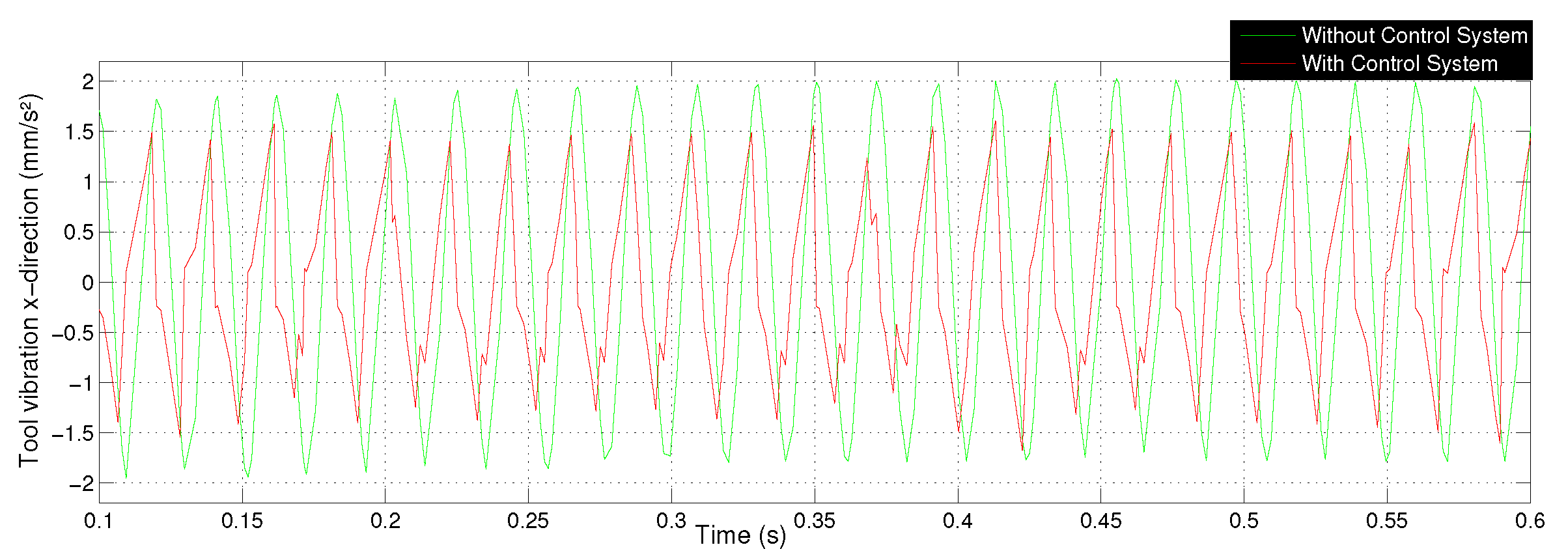
Matlab/Simulink is utilized as the software environment. Simulation results are presented to validate that the tool chatter can be mitigated significantly by implementing the combined technique of AVD and DSMC-T2 fuzzy. The proposed control strategy result is then compared with DSMC, D-PID, DSMC-T1 fuzzy to prove the capabilities of DSMC-T2 fuzzy in vibration mitigation. For the simulation process, a total duration of 0.1 s to 0.6 s is considered. The weight of the AVD is considered to be 5 % of the main device and this assumption is implemented in the simulation process. For the comparison of the results, two subsystem blocks of the milling model are developed using Simulink, where one block includes control systems and the other block has no control. The inputs to the process model are cutting forces and damper forces. The value 650 rad/s is set as the frequency of the simulation procedure. The arrangements of numerical integrators and filters are implemented to convert the acceleration signals to required velocities and positions. The four sets of tests are conducted with DSMC, with D-PID, with DSMC -T1 fuzzy and DSMC-T2 fuzzy for the generation and comparison of results. The toolbox named IT2-FLSs designed by Taksin et al. [55] is utilized for processing type-2 fuzzy operations. The membership functions selected for position error and velocity error are three and two, respectively. The process of normalization is carried out in the form [ 2 , 2 ] . The methodology implemented for the defuzzification of the type-2 fuzzy logic system is Karnik-Mendel technique [26]. In this paper, for the control of chatter considering the type-2 fuzzy logic concept, six fuzzy rules for j ^ as well as four fuzzy rules for h ^ are sufficient for effective control. Considering the type-1 fuzzy logic concept, for the control of chatter, nine fuzzy rules for j ^ and six fuzzy rules for h ^ are sufficient. The membership functions are designed using Gaussian function. IF–THEN rules are applied for both the types of fuzzy system.The chosen learning rates are Ω 1 = Ω 2 = 0.9 . Theorem 1 is utilized for selecting σ which is 0.17 .
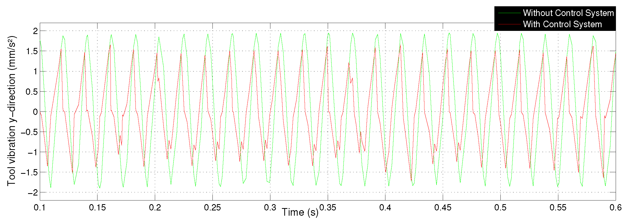
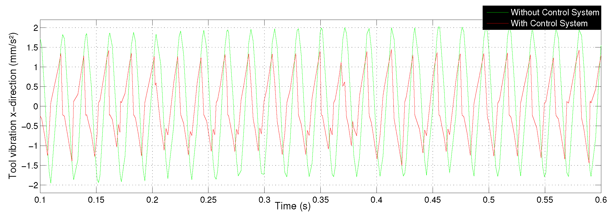
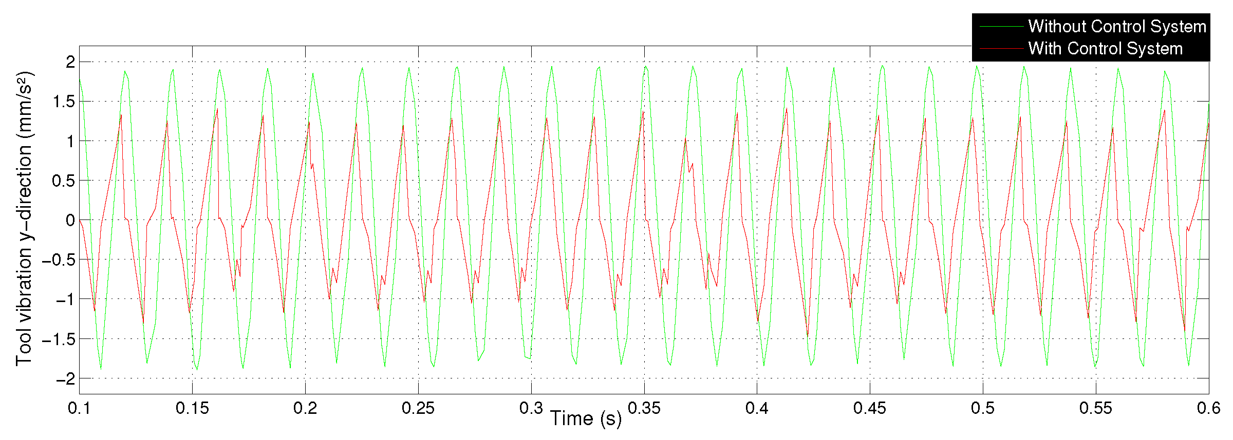
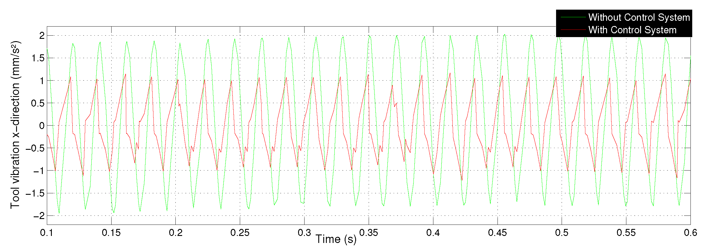
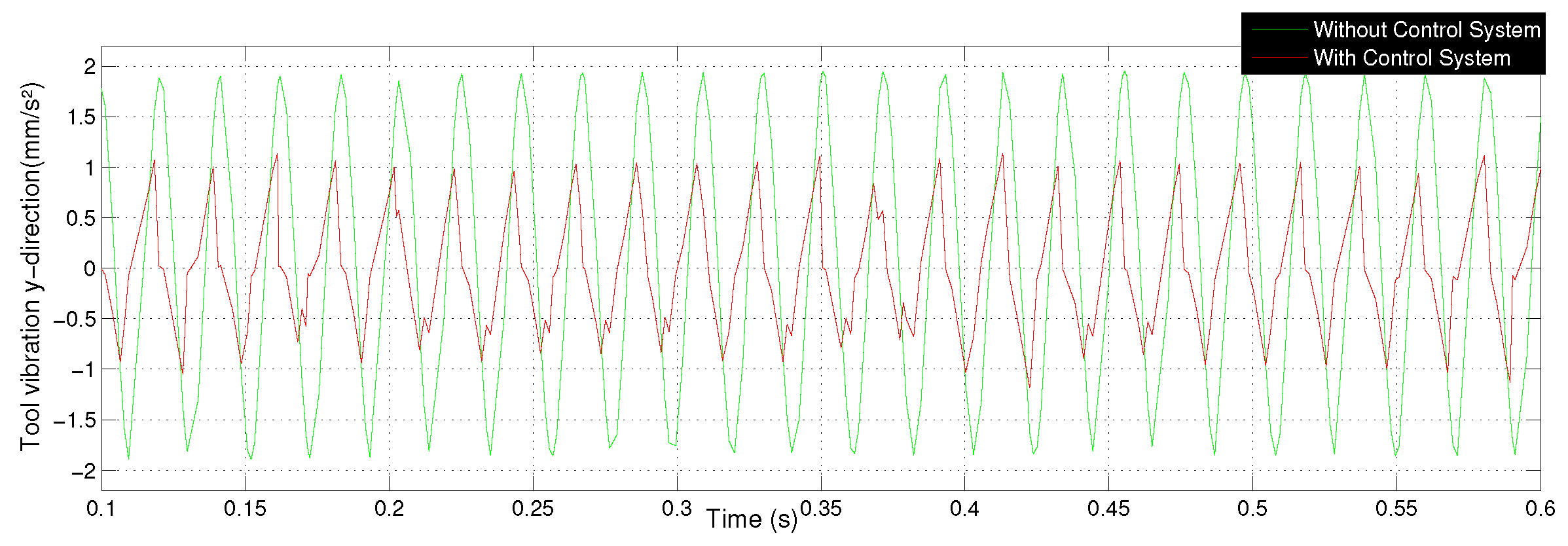
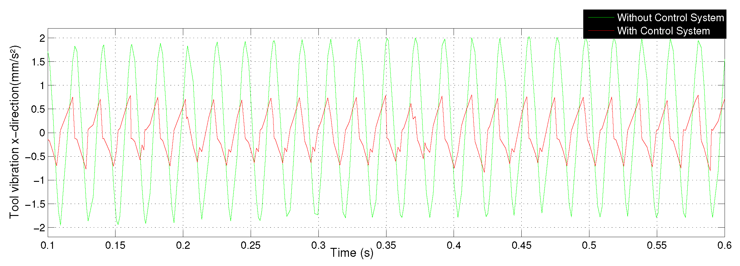
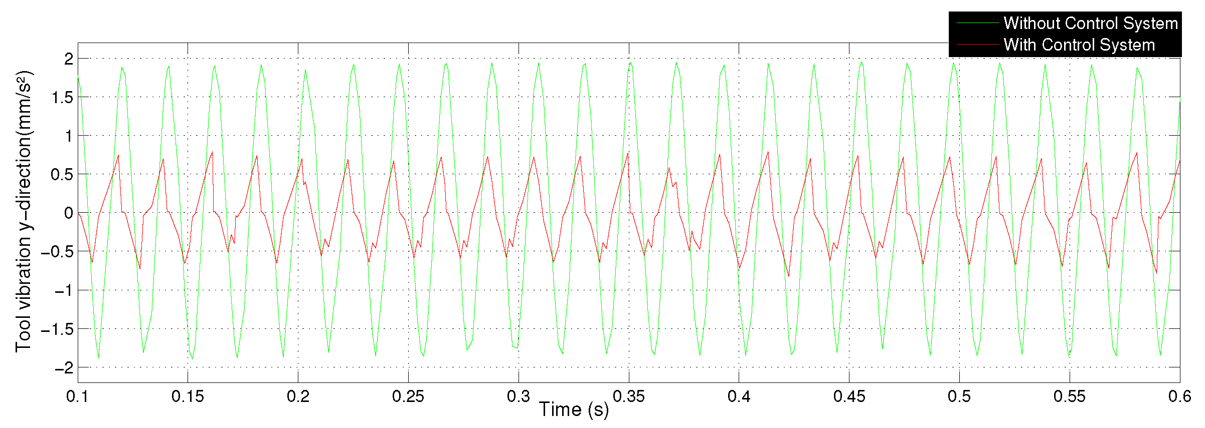
The vibration minimization obtained by implementing the controllers DSMC, D-PID, DSMC-T1 fuzzy and DSMC-T2 fuzzy are compared for validating the effectiveness and the results are shown in the plots given by Figure 4, Figure 5, Figure 6, Figure 7, Figure 8, Figure 9, Figure 10 and Figure 11. The equation mean squared error (MSE) = 1 d k = 1 d x k 2 is implemented to calculate the average vibration minimization results and is displayed in Table 2. In the equation, x k stands for chatter and d illustrates the total amount of data. In the Table 2, T1 is type-1 and T2 is type-2.
The results of percentage vibration minimization of all the controllers are calculated utilizing the MSE indicator. The percentage vibration mitigation using DSMC is 40.88 % along the x component and 36.46 % along the y component, whereas D-PID reduces the vibration by 51.58 % along the x component and 52.89 % along the y component. The percentage vibration mitigation using DSMC-T1 fuzzy is 70.20 % along the x component and 70.63 % along the y component. Finally, the percentage vibration mitigation using DSMC-T2 fuzzy is 79.02 % along the x component and 78.2 % along the y component. So it validated that the implementation of the type-2 fuzzy system in DSMC made it perform better than the DSMC-T1 fuzzy controller. The outcome of percentage vibration suppression depicts that the type-2 fuzzy system performed better than the type-1 fuzzy system. In general, the DSMC-T2 fuzzy controller performed better than all the controllers used in this research.
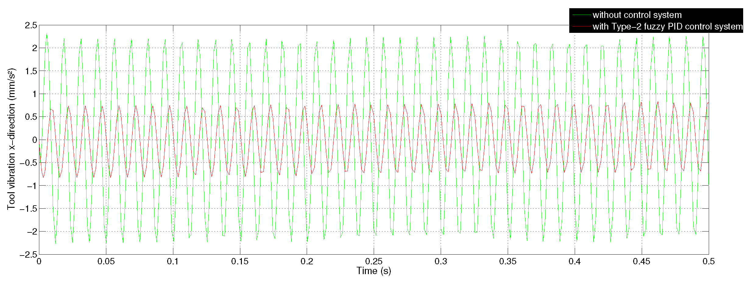
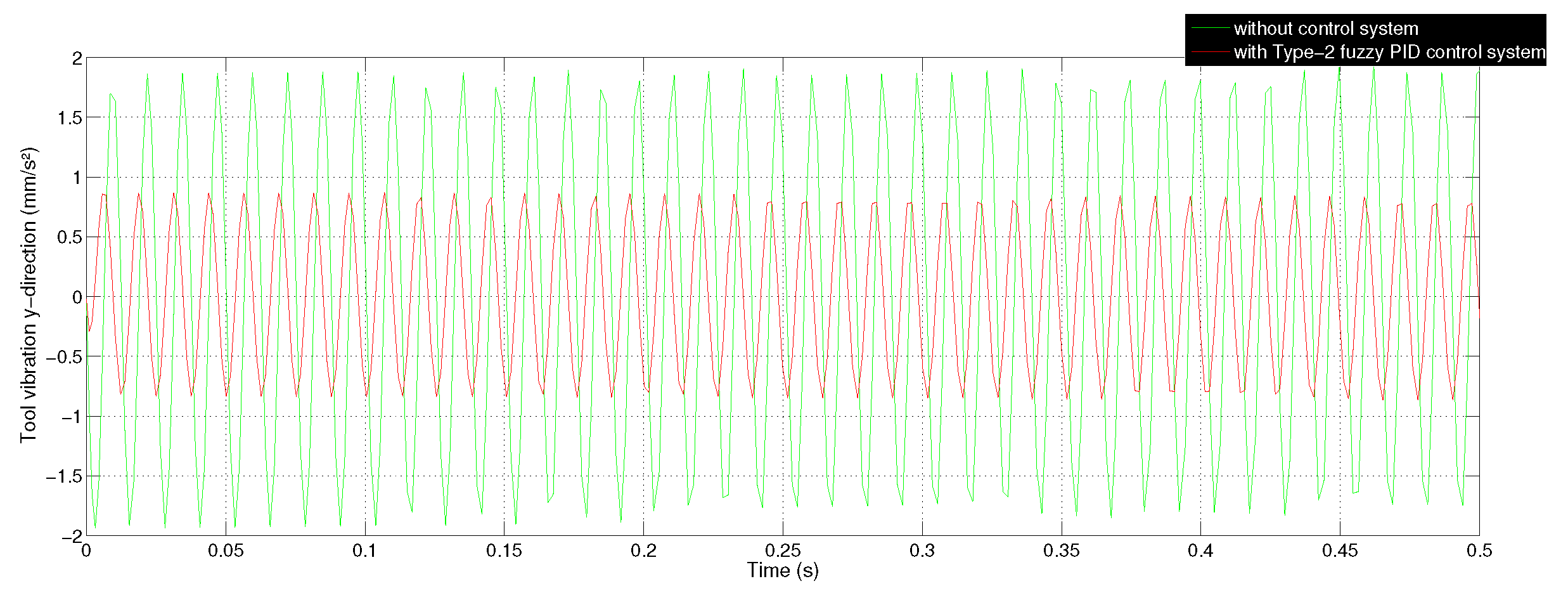
A type-2 fuzzy PID controller was used to mitigate the chatter vibration in the milling process [56]. The plots depicting the vibration attenuation using the type-2 fuzzy PID controller are illustrated in Figure 12 and Figure 13. The MSE results reveal that the average vibration attenuation with the type-2 fuzzy PID controller along the x-direction is 80 % in comparison to 79.02 % with DSMC-T2 fuzzy, whereas along the y-direction with the type-2 fuzzy PID controller is 76.3 % in comparison to 78.2 % with the DSMC-T2 fuzzy. So it is clear that both the controllers performed well and their performances are almost equal. The advantages of using DSMC-T2 fuzzy over type-2 fuzzy PID controller are: (a) It is effective in terms of robustness against the changes in the parameters with external disturbances and can be implemented without the knowledge of system parameters; (b) the computational cost of the type-2 fuzzy PID controller is bigger than the DSMC-T2 fuzzy.
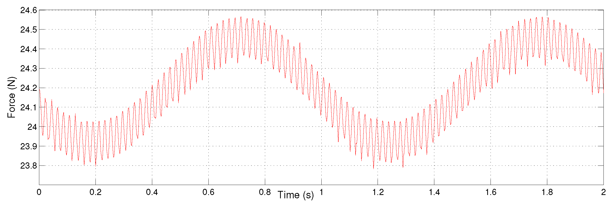
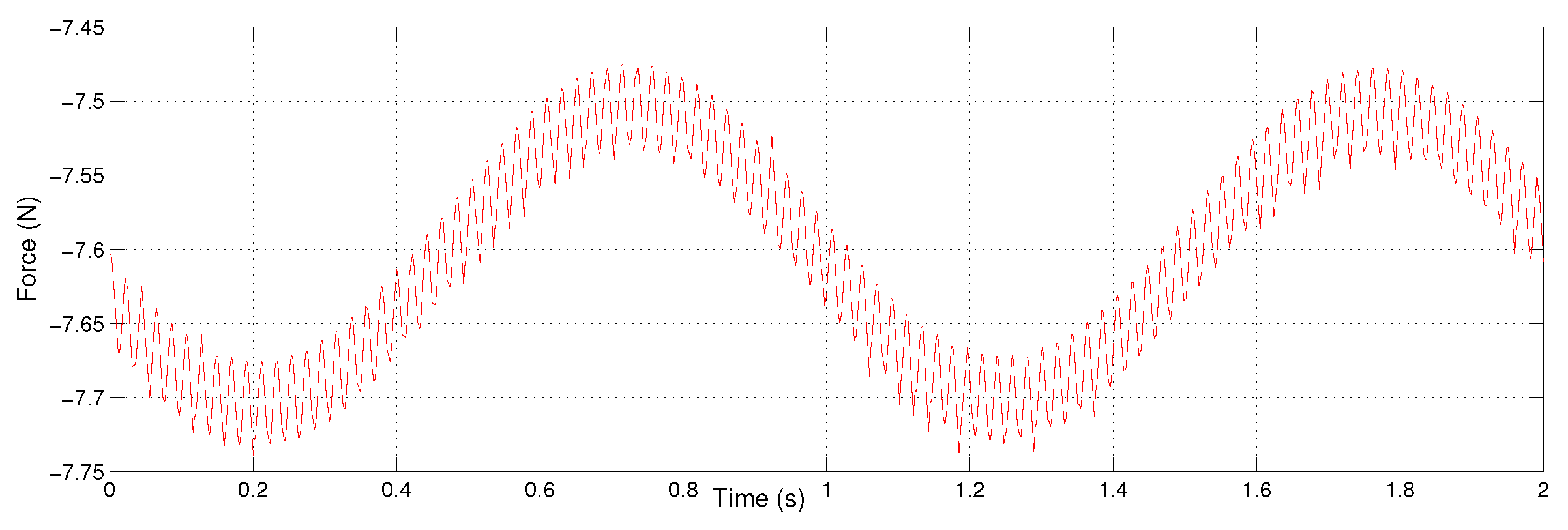
For superior vibration mitigation, it is very important to place the damper in a proper position. This work demands that the vibration attenuation should be accomplished along the x and y components and hence suitably two AVDs need to be installed along the x and y axes, separately. However, in this research, the setup is made cost effective by installing a single AVD in an inclined position to control the forces along the x and y axes. The cutting forces associated with the x and y axes are shown in Figure 14 and Figure 15, respectively. 
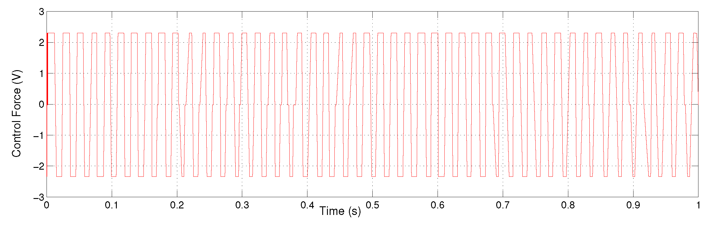
Figure 16 illustrates the behavior of the DSMC-type-2 fuzzy control signal.

5. Conclusions

In this paper, a novel technique for milling chatter mitigation is demonstrated using an active control strategy. In the first phase, the mathematical modeling of the process is carried out. The DSMC is combined with type-2 fuzzy logic for an effective control mechanism. Numerical analysis validated that the innovative controller is able to mitigate vibration significantly. Using the Lyapunov analysis technique, a theorem is laid down to prove that the system states of the DSMC-T2 fuzzy controller are bounded. An efficient approach of the type-2 fuzzy system is implemented to handle the nonlinearities in a suitable manner. The results from numerical analysis establish that the most superior controller is DSMC-T2 fuzzy. As the literature review suggests, SMC in combination with fuzzy is utilized for vibration control, but this combination along with stability analysis is not used for the milling process. In this paper, the stability of the controller is given due importance. The stability of the controller is validated using Lyapunov analysis. Moreover, the concept of implementing type-2 fuzzy logic for nonlinearity compensation in the milling process is done for the first time. Moreover, the research is made cost effective by placing the AVD in an inclined position. The higher computational cost is the primary concern associated with the toolbox of type-2 fuzzy logic and there is a need to deal with this situation with a suitable methodology. The techniques of minimizing the computational cost will be investigated in future work. Moreover, in future, an experimental setup will be developed to validate the theoretical concept. There is also the requirement of designing a torsional actuator for the control of chatter in the theta direction (torsional vibration).

Author Contributions

Conceptualization, S.P.; Methodology, S.P. and R.M.-M.; Software, S.P.; Validation, R.M.-M. and S.P.; Investigation, S.P.; Writing—original draft preparation, S.P.; Writing—review and editing, S.P. and R.M.-M.; Supervision, R.M.-M.; Project administration, R.M.-M.; Funding acquisition, R.M.-M. These authors contributed equally to this work.

Funding

This research was funded by Tecnológico de Monterrey, School of Engineering and Sciences, Monterrey, NL, Mexico.

Conflicts of Interest

The authors declare no conflict of interest.

References

  1. Rusinek, R.; Wiercigroch, M.; Wahi, P. Modelling of Frictional Chatter in Metal Cutting. Int. Mech. Sci. 2014, 89, 167–176. [Google Scholar] [CrossRef]
  2. Parus, A.; Powalka, B.; Marchelek, K.; Domek, S.; Hoffmann, M. Active Vibration Control in Milling Flexible Workpiece. J. Vib. Control 2013, 19, 1103–1120. [Google Scholar] [CrossRef]
  3. Venter, G.S.; Martins da Silva, M. An Analysis of Surface Roughness in Turning/Boring Under Different Chatter Conditions. In Proceedings of the 24th ABCM International Congress of Mechanical Engineering, Curitiba, Brazil, 3–8 December 2017. [Google Scholar]
  4. Erturk, A.; Inman, D. Piezoelectric Shunt Damping for Chatter Suppression in Machining Processes. In Proceedings of the ISMA, Leuven, Belgium, 15–17 September 2008. [Google Scholar]
  5. Venter, G.; Silva, L.; Carneiro, M.; Martins da Silva, M. Passive and Active Strategies Using Embedded Piezoelectric Layers to Improve the Stability Limit in Turning/Boring Operations. Int. Adv. Technol. 2017, 89, 2789–2801. [Google Scholar] [CrossRef]
  6. Ssffury, J.; Altus, E. Chatter Resistance of Non-Uniform Turning Bars with Attached Dynamic Absorbers-Analytical Approach. J. Sound Vib. 2010, 329, 2029–2043. [Google Scholar] [CrossRef]
  7. Yang, Y.; Dai, W.; Liu, Q. Design and Implementation of Two-Degree-of-Freedom Tuned Mass Damper in Milling Vibration Mitigation. J. Sound Vib. 2015, 335, 78–88. [Google Scholar] [CrossRef]
  8. Quintana, G.; Ciurana, J. Chatter in Machining Processes: A Review. Int. J. Mach. Tools Manuf. 2011, 51, 363–376. [Google Scholar] [CrossRef]
  9. Ganguli, A.; Deraemaeker, A.; Preumont, A. Regenerative Chatter Reduction by Active Damping Control. J. Sound Vib. 2007, 300, 847–862. [Google Scholar] [CrossRef]
  10. Harms, A.; Denkena, B.; Lhermet, N. Tool Adaptor for Active Vibration Control in Turning Operation. In Proceedings of the 9th International Conference on New Actuators, Bremen, Germany, 14–16 June 2004; pp. 694–697. [Google Scholar]
  11. Dohner, J.L.; Lauffer, J.P.; Hinnerichs, T.D.; Shankar, N.; Regelbrugge, M.; Kwan, C.-M.; Xu, R.; Winterbauere, B.; Bridgerf, K. Mitigation of Chatter Instabilities in Milling by Active Structural Control. J. Sound Vib. 2004, 269, 197–211. [Google Scholar] [CrossRef]
  12. Zhang, L.; Chen, M.Z.Q. Event-Based Global Stabilization of Linear Systems via a Saturated Linear Controller. Int. J. Robust Nonlinear Control 2015, 26, 1073–1091. [Google Scholar] [CrossRef]
  13. Chen, Z.; Zhang, H.-T.; Zhang, X.; Ding, H. Adaptive Active Chatter Control in Milling Processes. J. Dyn. Syst. Meas. Control 2014, 136, 021007. [Google Scholar] [CrossRef]
  14. Weremczuk, A.; Rusinek, R.; Warminski, J. The Concept of Active Elimination of Vibrations in Milling Process. Procedia CIRP 2015, 31, 82–87. [Google Scholar] [CrossRef] [Green Version]
  15. AlharbiI, W.N.; Batako, A.; Gomm, B. PID Controller Design for VIibratory Milling. In Proceedings of the ISER International Conference, Marrkech, Morocco, 13–14 July 2017. [Google Scholar]
  16. Melkote, S.N.; Endres, W.J. The Importance of Including Size Effect when Modeling Slot Milling. J. Manuf. Sci. Eng. 1998, 120, 68–75. [Google Scholar] [CrossRef]
  17. Stepan, G.; Kalmar-Nagy, T. Nonlinear Regenerative Machine Tool Vibrations. In Proceedings of the 16th ASME Biennial Conference on Mechanical Vibration and Noise, Sacramento, CA, USA, 14–17 September 1997; pp. 1–11. [Google Scholar]
  18. Kalmar-Nagy, T.; Stepan, G.; Moon, F.C. Subcritical Hopf Bifurcation in the Delay Equation Model for Machine Tool Vibrations. Nonlinear Dyn. 2001, 26, 121–142. [Google Scholar] [CrossRef]
  19. Dombovari, Z.; Wilson, R.E.; Stepan, G. Estimates of the Bistable Region in Metal Cutting, Proc. of the Royal Society of London A: Mathematical. Phys. Eng. Sci. 2008, 464, 3255–3271. [Google Scholar] [CrossRef]
  20. Moradi, H.; Bakhtiari-Nejad, F.; Movahhedy, M.R.; Vossoughi, G.R. Stability Improvement and Regenerative Chatter Suppression in Nonlinear Milling Process via Tunable Vibration Absorber. J. Sound Vib. 2012, 331, 4668–4690. [Google Scholar] [CrossRef]
  21. Liang, M.; Yeap, T.; Hermansya, A. A Fuzzy System for Chatter Suppression in End Milling. Proc. Inst. Mech. Part B J. Eng. Manuf. 2004, 218, 403–417. [Google Scholar] [CrossRef]
  22. Sims, N.D.; Manson, G.; Mann, B. Fuzzy Stability Analysis of Regenerative Chatter in Milling. J. Sound Vib. 2010, 329, 1025–1041. [Google Scholar] [CrossRef]
  23. Chadli, M.; Maquin, D.; Ragot, J. Static output feedback for Takagi-Sugeno systems: An LMI approach. In Proceedings of the 10th Mediterranean Conference on Control and Automation, Lisbonne, Portugal, 9–13 July 2002. [Google Scholar]
  24. Barnes, M.R. Neuro-Fuzzy Clustering of Radiographictibia Image Data Using type-2 Fuzzy Sets. Inf. Sci. 2000, 125, 65–82. [Google Scholar]
  25. Mendel, J.M. Uncertain Rule-Based Fuzzy Logic Systems: Introduction and New Directions; Prentice Hall PTR: Upper Saddle River, NJ, USA, 2001. [Google Scholar]
  26. Liang, Q.; Mendel, J.M. Interval type-2 Fuzzy Logic Systems: Theory and Design. IEEE Trans. Fuzzy Syst. 2002, 8, 535–550. [Google Scholar] [CrossRef]
  27. Sepúlveda, R.; Castillo, O.; Melin, P.; Rodríguez-Díaz, A.; Montiel, O. Experimental Study of Intelligent Controllers Under Uncertainty using type-1 and type-2 Fuzzy Logic. Inf. Sci. 2007, 177, 2023–2048. [Google Scholar]
  28. Hassani, H.; Zarei, J.; Chadli, M.; Qiu, J. Unknown Input Observer Design for Interval type-2 T–S Fuzzy Systems With Immeasurable Premise Variables. IEEE Trans. Cybern. 2017, 47, 2639–2650. [Google Scholar] [CrossRef] [PubMed]
  29. Paul, S.; Yu, W.; Li, X. Bidirectional active control of structures with type-2 fuzzy PD and PID. Int. J. Syst. Sci. 2018, 49, 766–782. [Google Scholar] [CrossRef]
  30. Naik, K.A.; Gupta, C.P. Performance comparison of type-1 and type-2 fuzzy logic systems. In Proceedings of the 4th International Conference on Signal Processing, Computing and Control (ISPCC), Solan, India, 21–23 September 2017; pp. 72–76. [Google Scholar]
  31. Bai, Y.; Wang, D. On the Comparison of type-1 and Interval type 2 Fuzzy Logic Controllers Used in a Laser Tracking System. IFAC-PapersOnLine 2018, 51, 1548–1553. [Google Scholar] [CrossRef]
  32. Utkin, V.I. Sliding Modes in Control and Optimization; Springer: Berlin, Germany, 1992. [Google Scholar]
  33. Moradi, H.; Movahhedy, M.R.; Vossoughi, G. Sliding Mode Control of Machining Chatter in the Presence of Tool Wear and Parametric Uncertainties. J. Vib. Control. 2009, 16, 231–251. [Google Scholar] [CrossRef]
  34. Zhao, P.; Shi, Y.; Huang, J. Proportional-integral based fuzzy sliding mode control of the milling head. Control. Eng. Pract. 2016, 53, 1–13. [Google Scholar] [CrossRef]
  35. Ma, H.; Wu, J.; Yang, L.; Xiong, Z. Active chatter suppression with displacement-only measurement in turning process. J. Sound Vib. 2017, 401, 255–267. [Google Scholar] [CrossRef]
  36. Nguyen, S.D.; Kim, W.; Park, J.; Choi, S.-B. A new fuzzy sliding mode controller for vibration control systems using integrated-structure smart dampers. Smart Mater. Struct. 2017, 26, 045038. [Google Scholar] [CrossRef]
  37. Phu, D.X.; Quoc, N.V.; Park, J.-H.; Choi, S.-B. Design of a novel adaptive fuzzy sliding mode controller and application for vibration control of magnetorheological mount. Proc. Institution Of Mech. Eng. Part C J. Mech. Eng. Sci. 2014, 228, 2285–2302. [Google Scholar] [CrossRef]
  38. Çetin, Ş.; Akkaya, A.V. Simulation and hybrid fuzzy-PID control for positioning of a hydraulic system. Nonlinear Dyn. 2010, 61, 465–476. [Google Scholar] [CrossRef]
  39. Yong, Y.; Rydberg, K.; An, L. An improved PI control for active damping of a hydraulic crane boom system. In Proceedings of the ICMIT 2005: Control Systems and Robotics, Chongqing, China, 20–23 September 2005. [Google Scholar]
  40. Zhang, H.-T.; Wu, Y.; He, D.; Zhao, H. Model Predictive Control to Mitigate Chatters in Milling Processes with Input Constraints. Int. J. Mach. Tools Manuf. 2015, 91, 54–61. [Google Scholar] [CrossRef]
  41. Liu, X.; Su, C.Y.; Li, Z.; Yang, F. Adaptive Neural-Network-Based Active Control of Regenerative Chatter in Micromilling. IEEE Trans. Autom. Sci. Eng. 2018, 15, 628–640. [Google Scholar] [CrossRef]
  42. Van Dijk, N.J.M.; van de Wouw, N.; Doppenberg, E.J.J.; Oosterling, H.A.J.; Nijmeijer, H. Robust Active Chatter Control in the High-Speed Milling Process. IEEE Trans. Control. Syst. Technol. 2012, 20, 901–917. [Google Scholar] [CrossRef]
  43. Altintas, Y.; Stepan, G.; Merdol, D.; Dombovari, Z. Chatter Stability of Milling in Frequency and Discrete Time Domain. CIRP J. Manuf. Sci. Technol. 2008, 1, 35–44. [Google Scholar] [CrossRef]
  44. Roldán, C.; Campa, F.J.; Altuzarra, O.; Amezua, E. Automatic Identification of the Inertia and Friction of an Electromechanical Actuator. In New Advances in Mechanisms, Transmissions and Applications; Series Mechanisms and Machine Science; Springer: Dordrecht, The Netherlands, 2014; Volume 17, pp. 409–416. [Google Scholar]
  45. Sarhan, A.A.D.; Matsubara, A. Investigation about the characterization of machine tool spindle stiffness for intelligent CNC end milling. Robot. Comput.-Integr. Manuf. 2015, 34, 133–139. [Google Scholar] [CrossRef]
  46. Sarhan, A.A.D.; Matsubara, A.; Sugihara, M.; Saraie, H.; Ibaraki, S.; Kakino, Y. Monitoring Method of Cutting Force by Using Additional Spindle Sensors. JSME Int. J. Ser. Mech. Mach. Elem. Manuf. 2006, 49, 307–315. [Google Scholar] [CrossRef] [Green Version]
  47. Lee, C.S.; Hong, H.P. Statistics of inelastic responses of hysteretic systems under bidirectional seismic excitations. Eng. Struct. 2010, 32, 2074–2086. [Google Scholar] [CrossRef]
  48. Kim, J.; Oh, S.; Cho, D.; Hedrick, J. Robust Discrete-Time Variable Structure Control Methods. ASME J. Dyn. Sys. Meas. Control 2000, 122, 766–775. [Google Scholar] [CrossRef]
  49. Ding, Y.; Zhu, L.; Zhang, X.; Ding, H. A full-discretization method for prediction of milling stability. Int. Mach. Tools Manuf. 2010, 50, 502–509. [Google Scholar] [CrossRef]
  50. Horn, R.A.; Johnson, C.R. Matrix Analysis; Cambridge University Press: Cambridge, UK, 1985. [Google Scholar]
  51. Ioannou, P.; Sun, J. Robust Adaptive Control; Prentice-Hall: Upper Saddle River, NJ, USA, 1996. [Google Scholar]
  52. Moradi, H.; Movahhedy, M.R.; Vossoughi, G. Dynamics of Regenerative Chatter and Internal Resonance in Milling Process with Structural and Cutting Force Nonlinearities. J. Sound Vib. 2012, 331, 3844–3865. [Google Scholar] [CrossRef]
  53. De Cock, K.; De Moor, B.; Minten, W.; Van Brempt, W.; Verrelst, H. A Tutorial on PID-Control; ESAT-SISTA/TR 1997-08; Katholieke Universiteit Leuren Department of Electrical Eng: Leuren, Belgium, 1997. [Google Scholar]
  54. Chander, S.; Agarwal, P.; Gupta, I. Auto-tuned, discrete PID controller for DC-DC converter for fast transient response. In Proceedings of the India International Conference on Power Electronics 2010 (IICPE2010), New Delhi, India, 28–30 January 2011; pp. 1–7. [Google Scholar]
  55. Taskin, A.; Kumbasar, T. An Open Source Matlab/Simulink Toolbox for Interval type-2 Fuzzy Logic Systems. In Proceedings of the IEEE Symposium Series on Computational Intelligence, Cape Town, South Africa, 7–10 December 2015; Volume 1, pp. 1561–1566. [Google Scholar]
  56. Paul, S.; Morales-Menendez, R. Active Control of Chatter in Milling Process Using Intelligent PD/PID Control. IEEE Access 2018, 6, 72698–72713. [Google Scholar] [CrossRef]
Figure 1. Illustration of milling process dynamics [42,43].
Applsci 09 04380 g001
Figure 2. AVD on Spindle Top.
Applsci 09 04380 g002
Figure 3. Brief overview of control process.
Applsci 09 04380 g003
Figure 4. Tool vibration along x-direction using DSMC.
Applsci 09 04380 g004
Figure 5. Tool vibration along y-direction using DSMC.
Applsci 09 04380 g005
Figure 6. Tool vibration along x-direction using D-PID.
Applsci 09 04380 g006
Figure 7. Tool vibration along y-direction using D-PID.
Applsci 09 04380 g007
Figure 8. Tool vibration along x-direction using DSMC-T1 fuzzy.
Applsci 09 04380 g008
Figure 9. Tool vibration along y-direction using DSMC-T1 fuzzy.
Applsci 09 04380 g009
Figure 10. Tool vibration along x-direction using DSMC-T2 fuzzy.
Applsci 09 04380 g010
Figure 11. Tool vibration along y-direction using DSMC-T2 fuzzy.
Applsci 09 04380 g011
Figure 12. Tool vibration along x - direction using type-2 Fuzzy PID control.
Applsci 09 04380 g012
Figure 13. Tool vibration along y - direction using type-2 Fuzzy PID control.
Applsci 09 04380 g013
Figure 14. Cutting force along x-direction.
Applsci 09 04380 g014
Figure 15. Cutting force along y-direction.
Applsci 09 04380 g015
Figure 16. Control signal of DSMC with type-2 fuzzy logic.
Applsci 09 04380 g016
Table 1. Parameters.
ParameterValueUnitsParameterValueUnits
m x 20kg m y 20kg
c x 1200Ns/m c y 4300Ns/m
k x 7.2 × 10 6 N/m k y 6.48 × 10 7 N/m
ξ 1 6700 × 10 9 N / m 3 δ 1 13,000 × 10 9 N / m 3
ξ 2 4900 × 10 6 N / m 2 δ 2 7200 × 10 6 N / m 2
ξ 3 3000 × 10 3 N/m δ 3 13N
ξ 4 1700 × 10 3 N/m δ 4 25N
n4 Ω 3000 r e v / min
Table 2. Average vibration attenuation, mean squared error (MSE) indicator.
DirectionNo ctrl.DSMCD-PIDDSMC-T1 FuzzyDSMC-T2 Fuzzy
x-direction 0.3823 0.2260 0.1851 0.1172 0.0802
y-direction 0.3702 0.2352 0.1744 0.1087 0.0807

