Abstract
The traditional mean squared error (MSE) criterion can be formulated as a quadratic function of a vector of control filter coefficients, and it is easy to obtain optimal control filter coefficients. Although the MSE criterion can lead to noise reductions in the control area, an unpredictable directional residual sound field is generated. In this paper, we propose a method for multi-channel active harmonic noise control with a local minimax error criterion based on the Nelder–Mead algorithm, which leads to reductions at all error positions and greater reductions at controllable positions. Directional noise reduction experiments of two areas are presented for two different error criteria at discrete locations in an anechoic chamber. Compared with a system employing the traditional MSE criterion, the results show that an active noise control system with the proposed criterion can achieve extra reductions at specified locations and overall noise reductions at the same time. The present research offers some important insights into directional control.
1. Introduction
Currently, acoustic noise problems are very serious as more noise sources, such as car engines, fans, transformers, and compressors, emerge. Noise control technology can be divided into two categories: passive and active noise control [1]. Passive control, such as enclosures, barriers, and silencers, are no longer practically effective at low frequencies. Active noise control (ANC) can offset the primary noise source, by adding a secondary source, which has an equal amplitude and opposite phase at the control point based on the principle of superposition. ANC has shown the great control performance at low frequencies. Until now, ANC has been successfully applied in many areas. Studies have shown that ANC can be used to control the noise associated with air-craft fuselages, automobile interiors, and open windows [2,3,4,5,6,7].
ANC systems can be divided into two categories based on two control strategies, feedforward control and feedback control [8]. Feedforward control is more robust than the feedback control since feedforward control has a coherent reference signal as the input of the controller, which is more stable in terms of control performance [9]. However, possible acoustic feedback from secondary sources to reference sensors arises in the feedforward control, destroying the noise reduction effect. Traditionally, the use of non-acoustic sensors or directional microphones and speakers can avoid the acoustic feedback phenomenon. A neutralization method has been proposed to solve this problem by subtracting the acoustic feedback from the signal detected by the reference microphone. Like the infinite impulse response (IIR) controller, the neutralization method can generate a pole, producing an instability in the control system [10].
A complex noise field requires a multi-channel strategy to meet the desired demands of noise reduction. Traditionally, when the mean squared error (MSE) criterion is adopted to calculate optimal filter coefficients, a multi-channel system can achieve a good performance in terms of noise reduction. However, the residual acoustic field will generate an unpredictable directivity, due to the large differences between the maximum and minimum levels of the residual sound field [11]. Here, we can expect the noise reductions at all error points and hope for better reductions at certain locations. Previous work has reported much effort dedicated to active directivity control of the radiated sound. These methods are roughly divided into two categories: methods that use special speakers and methods that choose an appropriate error criterion.
A parametric loudspeaker array (PLA) is a special kind of speaker that generates a directional sound beam from the interaction of ultrasonic beams in the sound control field [12]. When we adopt a PLA in multi-channel ANC, the computational complexity of the algorithm is greatly reduced, since crosstalk secondary path models can be removed [13]. Tanaka used a PLA as the secondary source to avoid spillover phenomena and achieved noise control when an obstacle existed between the PLA and target points [14]. In addition, a moving directional ANC system was achieved by Tanaka [15]. The system adopted a steerable PLA based on a phased array rather than mechanically rotating the PLA, enabling the generation of a moving quiet zone. A problem with the PLA arrangement is nonlinear distortions, which have been the primary technical barriers to promoting PLAs’ application [16]. Although an ANC system with a PLA can mitigate sound locally, the system has little influence on the circumferential field.
Qiu and Zhao adopted a weighted sum of the squared sound pressures within an angle at error points as a cost function and achieved a directivity control from the near field to the far field [17]. Wang and Sun also proposed using a similar weighted sum of error signals based on the spatial Fourier transform as the error criterion [18]. Apart from Qiu and Zhao, Wang and Sun used a planar microphone array, perpendicular to the desired control direction. In addition, the input of the active controller was the sum of the error signals of the array, which was equivalent to a single channel and minimized the complexity of the ANC system. Like the above methods, weighted sum methods show less potential for reductions at other positions.
As mentioned above, ANC with the MSE method produces a residual acoustic field that can exhibit large differences between its maximum and minimum levels, producing a directivity. Gonzalez originally proposed an iterative minimax error criterion to produce the acoustic field in an enclosure that was more uniform than that achieved with the classic MSE criterion [11]. An iterative algorithm was developed that minimizes the maximum value of each of the error signals. In this approach, only the error microphone with the highest level is considered to design the ANC controller in each iteration, which reduces the computational load compared with that of the conventional least mean squares (LMS) algorithm. Fan used an iterative algorithm to design an active T-shaped noise barrier and obtained a uniform residual sound field [19]. To implement an iterative algorithm based on a minimax error criterion in real applications, Shi adopted the partial update (P-U) minimax algorithm and modified the iterations, further reducing the computational load [20].
Previous methods cannot balance the reductions at the desired points and those at other locations. To solve this problem, we introduce a local minimax error based on the Nelder–Mead algorithm as a new criterion. Given the computational complexity and stability of real-time processing in an ANC system, a fixed controller is designed offline with the proposed method. A controllable directional reduction and an overall reduction can be realized by minimizing the maximum error of certain points.
The remainder of the paper is organized in five sections. Section 2 derives a fixed optimal filter that is designed by the MSE criterion in a feedforward multi-channel system. Section 3 describes a fixed optimal filter designed with the local minimax error criterion based on the Nelder–Mead algorithm in a feedforward multi-channel system. Section 4 introduces the experimental setup. Section 5 shows the performance of the two error criteria. Experimental results are presented and discussed. In addition, conclusions are provided in Section 6.
2. Design of a Fixed Optimal Filter in the Frequency Domain with the Mean Squared Error Criterion
A block diagram of a feedforward multi-channel system with a single reference signal in the frequency domain at frequency w is shown in Figure 1 [21].
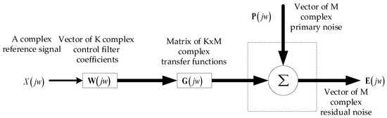
Figure 1.
Block diagram of a feedforward multi-channel system with a single reference signal in the frequency domain.
Based on acoustic superposition, the residual noise at frequency w can be expressed as:
where the superscript T indicates a transpose operation. is the complex reference signal; is a column vector of K complex control filter coefficients; is a matrix of complex transfer functions; and is a row vector of M complex primary noise. To be concise, the variable is omitted and:
The MSE criterion can be expressed as:
where the superscript H is the Hermitian operator. According to Equation (3), the sum-of-the-squared of residual noise at discrete locations can be formulated as a quadratic function of the vector . The optimal solution of the sum of the squared residual noise at error points can be found directly by differentiating Equation (3) with respect to and setting the gradient equal to zero. The result of the operation is:
3. Design of a Fixed Optimal Filter in the Frequency Domain with the Local Minimax Error Criterion
Based on the local minimax error criterion, can be described as:
where is the infinite norm, and the subscript d represents certain discrete points at which better reductions are desired. is also a function of the vector . The traditional minimax error criterion deduced can be expressed as [21]:
where represents the residual noise at all error points. is guaranteed to be convex and has a unique global minimum that can be obtained by an iterative gradient descent algorithm. Obviously, such an algorithm is not suitable for the optimization of the local minimax error since we want to obtain reductions at other points. A feasible approach to achieve this goal is to optimize locally. Generally, initial values and algorithms play important roles in local optimizations [22]. The Nelder–Mead algorithm, using a derivative-free method, is employed to find the local minimum value of . The starting point is critical and can greatly affect the objective value of the local solution. A known point, but not the best, is often chosen as the initial values. In this paper, is employed to improve the performance of the original . Therefore, can be set as the initial values of . It is worth mentioning that the initial point of the Nelder–Mead algorithm is specified as a real vector in this method, whereas consists of complex numbers. Therefore, should be constructed as:
The Nelder–Mead algorithm, also called the downhill simplex method, is a direct search method in which the derivatives may not be known [23]. It is a heuristic search method that can converge to non-stationary points. The algorithm starts off with a randomly-generated simplex. After many iterations, the vertex of the simplex that yields that best objective value is returned. More details are available in [24]. A flowchart of an iteration in the algorithm is shown in Figure 2. The method uses the concept of a simplex, which is a special polytope of vertices in n dimensions. The starting points are , and the aim is to minimize . The iteration can be described as follows:
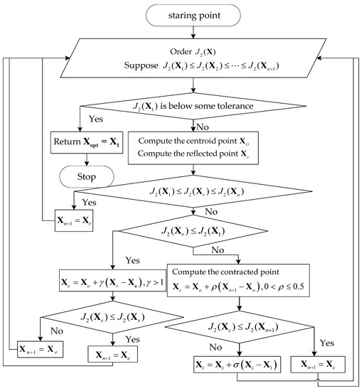
Figure 2.
An iteration in the Nelder–Mead algorithm.
Step 1. Order at the vertices : suppose . If is below some tolerance, and return the , which is expressed as .
Step 2. Compute , the centroid of all points except .
Step 3. Compute the reflected point, . If , . Therefore, a new simplex is generated; return to Step 1. If , . Then, if , ; otherwise, . Thus, a new simplex is generated; return to Step 1.
Step 4. Compute the contracted point, . If , . Thus, a new simplex is generated; return to Step 1.
Step 5. Replace all points except with . Thus, a new simplex is generated; return to Step 1.
Note: , and are the reflection, expansion, contraction, and shrink coefficients, respectively. The standard values are , and .
4. Experimental Setup
In this section, the experimental setup is explicitly introduced. The geometric configuration of the experiment can be seen in Figure 3.
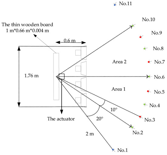
Figure 3.
Geometric configuration of the experiment.
The setup involved an actuator (a 44-mm resonant speaker), an array of loudspeakers (Swans, monitor-level active speaker, China), microphones (Brüel&Kjæ, 4189-A-021, Denmark), a thin wooden board (1 m × 0.6 × 0.004 m), a digital signal processing (DSP) development board (TI, TMS320C6678, USA), a power amplifier, an analogue-to-digital (A/D) converter (Maxim, max11049, USA), and a digital-to-analogue (D/A) converter (TI, dac764, USA). The actuator was directly attached to the center of the board and excited the board, producing harmonic noise at 100 Hz. Four speakers were used as secondary sources and were arranged 60 cm in front of the board. Eleven microphones, serving as the desired, monitor, or error points, surrounded the primary and secondary sources.
Directional noise reduction experiments were carried out in two areas. Microphones No. 2, No. 4, and No. 6 constituted the desired Area 1, where we wanted higher reductions. Microphones No. 3 and No. 5 were the monitor points in Area 1. Microphones No. 1, No. 8, No. 10, and No. 11 were other error points where we also expected reductions. Desired Area 2 consisted of Microphones No. 6, No. 8, and No. 10, where Microphones No. 7 and No. 9 were the corresponding monitor points and Microphones No. 1, No. 2, No. 4, and No. 11 were the remaining error points. Detailed distance and angle parameters can be found in Figure 3.
Considering the amount of calculation required in a practical application, the fixed controller was embedded in the DSP development board. The experiment was conducted with the following steps, as shown in Figure 4.
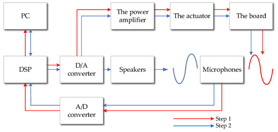
Figure 4.
Flow diagram of the experiment.
Step 1. Computation of the frequency domain transfer functions and recording of the primary noise field . The DSP development board generated a harmonic signal and passed the signal to the power amplifier through the D/A converter. The actuator received the amplified signal and excited the board. The microphones obtained the primary noise field at error points and passed it to the DSP development board through the A/D converter. Then, and were sent to the personal computer (PC). Therefore, the frequency-domain transfer functions can be calculated:
Optimal filter coefficients in the frequency domain of the methods, respectively mentioned in Section 2 and Section 3, and in the time domain can be obtained by a discrete inverse Fourier transformation.
Step 2. ANC. Firstly, the optimal filter coefficients in Step 1 were loaded on the DSP development board from the PC. The amplified harmonic signal from the DSP development board excited the board again. At the same time, the original signal was also the reference input of the optimal controller filter on the DSP development board. Finally, the outputs of the controller after the D/A converter were the inputs of the loudspeakers, producing the secondary field, ensuring that the residual noise of the arc discrete control points satisfied the relevant error criterion.
5. Experimental Results and Discussion
In this section, an experimental evaluation of the ANC system based on the two criteria is presented. A panoramic view of the experimental environment is shown in Figure 5.
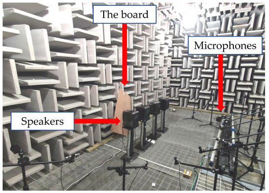
Figure 5.
Panoramic view of the experimental environment.
The board was positioned obliquely on the wire mesh to reduce the friction with the wire mesh when excited by the actuator in the anechoic chamber. The frequency of the original harmonic signal generated from the DSP board was 100 Hz. We conducted seven experiments as mentioned in Section 4, respectively in two different directional areas. The mean and standard deviation values were calculated to generate the error bar diagrams. The results of the experiments are presented in Figure 6.
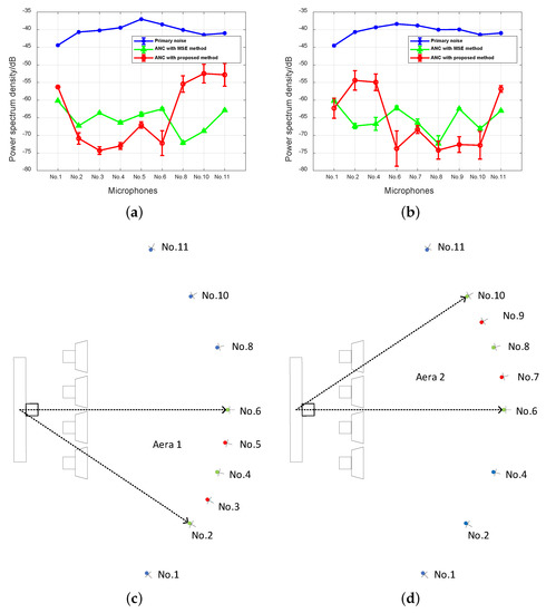
Figure 6.
Noise control performance of the two methods with two directional areas. (a) Active noise control (ANC) performance of the two methods with Directional Area 1; (b) ANC performance of the two methods with Directional Area 2; (c) Geometric configuration of the experiments with Directional Area 1. The points in green, red, and blue are the desired, monitor, and the rest of the error microphones points, respectively; (d) Geometric configuration of the experiments with Directional Area 2. The points in green, red, and blue are the desired, monitor, and the rest of the error microphones points, respectively.
An uncontrollable directivity was formed at Point No. 8 in Figure 6a and in Figure 6b when the MSE method was adopted. The directional reductions of Area 1 and Area 2 were achieved with the local minimax method, where Points No. 2, No. 4, and No. 6 and No. 6, No. 8, and No. 10 were the desired points of Area 1 and Area 2, respectively. Points No. 3, No. 5, No. 7, and No. 9 were the monitor points of the two areas. Similar to the global minimax method, the proposed method also led to a uniform residual sound at the desired points. The comparison with the MSE criterion method showed that an increase in the reduction in the directional area was accompanied by a reduction in the orthogonal direction, which was due to the choice of desired error points and the optimization algorithm. The local minimax criterion method aims to achieve the reductions at local points rather than all error microphones. Moreover, the local criterion optimization based on the Nelder–Mead algorithm with a known initial point can balance reductions between the local and global area, avoiding no reduction in orthogonal directions. It is worth noting that the standard deviations of the residual sound curves of the proposed method were larger than those of the two other curves in both figures. The effect of , , and can be ignored, according to Equation (1). It is very likely that this effect was caused by the floating variation of . A comparison of two optimal filter coefficients with two directional areas is presented in Figure 7.
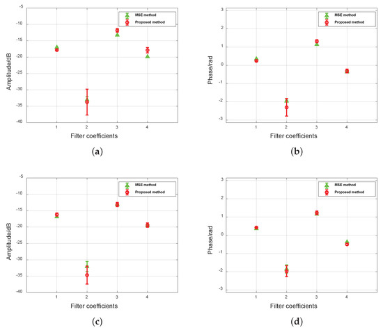
Figure 7.
Comparison of two optimal filter coefficients with two directional areas. (a) Comparison of the amplitude of filter coefficients with Directional Area 1. (b) Comparison of the phase of filter coefficients with Directional Area 1. (c) Comparison of the amplitude of filter coefficients with Directional Area 2. (d) Comparison of the phase of filter coefficients with Directional Area 2.
Similarly, the amplitude and phase curves of the local minimax method also had larger standard deviations. In Section 3, we mentioned that was obtained by a local optimization using as the initial value. The Nelder–Mead algorithm is a heuristic search method that will likely converge to non-stationary points. This means that the algorithm has the same problem, and different initial conditions could produce different results in each run. Therefore, a slight change resulting from the measurement error and calculation error in the calculation of may cause to change greatly. Fortunately, larger fluctuations in do not adversely affect the results of the algorithm. The overall reductions of the two methods are shown in Figure 8, where the floating change of the reductions was already explained.
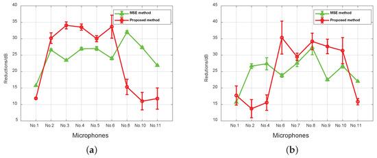
Figure 8.
The overall noise control performance of the two methods with two directional areas. (a) The overall reductions of the two methods with the Directional Area 1. (b) The overall reductions of the two methods with the Directional Area 2.
The parameters , , and are the average power spectrum density of primary noise, residual noise with the MSE method, and local minimax method obtained in the experiments. Now, we compare the reductions of the two methods at the desired, monitor and all error points. Compared with the reduction of ANC system with the MSE method, the extra noise reduction at the desired points and the extra noise reduction at the monitor point can be expressed in local terms as:
where and are the average power spectrum density of two residual noise at the desired points.
where and are the average power spectrum density of the two residual noise at the monitor points. The minimum of overall reductions with the proposed method can be expressed in global terms as:
The values of the parameters mentioned above in the experiments are shown in Table 1.

Table 1.
Values of reduction parameters.
In summary, the ANC system with the proposed method can achieve an extra 7.8-dB reduction at desired points and a 15.1-dB reduction overall when controlling Area 1, as well as an extra 9.8-dB reduction at desired points and a 15.5-dB reduction overall when controlling Area 2. The reductions of monitor points were respectively 3.5 dB and 5.9 dB, indicating the extent of the controlled area. The results showed that the system can realize directional reductions in a specified area with overall reductions, as well.
6. Conclusions
To achieve a directional noise reduction, as well as an overall noise reduction, this paper presented a local minimax error criterion that can balance local and global reductions with the optimization of the Nelder–Mead algorithm. The initial values of the traditional method were set as the starting points of the local optimization. Analyses were conducted for the dynamic residual sound, which resulted from the changes in the initial values. Based on the initial values of the traditional method, the new error criterion produced a satisfactory result, meeting the mentioned performance requirements. This research shed new light on the balanced ANC system.
Future works should focus on the following problems. First, to get a stable solution of the Nelder–Mead algorithm, stable initial values should be guaranteed. Second, remote microphone technology should be adopted when it is impossible to position microphones at a distance. Third, adaptive control and online identification are required for complex and variable sound environments.
Author Contributions
The author gratefully acknowledges the co-authors for their support and contribution to this work. K.C. and M.W. conceived of the work; R.H. helped with the Nelder–Mead algorithm; K.C. and C.G. conducted the experiments; M.W. and J.Y. are K.C.’s thesis supervisors and provided critical comments and guidance for the work. All authors have given final approval of the version to be published.
Acknowledgments
This work was supported by the National Key Research and Development Program of China (Grant No. 2016YFB1200503) and the National Natural Science Foundation of China (Grant No. 11474306, No. 11404367, and No. 11474307).
Conflicts of Interest
The authors declare no conflict of interest.
References
- Kuo, S.M.; Morgan, D.R. Active Noise Control Systems: Algorithms and DSP Implementations, 1st ed.; Wiley-Interscience: New York, NY, USA, 1996; pp. 1–2. [Google Scholar]
- Johansson, S. Active Control of Propeller-Induced Noise in Aircraft Algorithms & Methods; OCLC: 943545802; Blekinge Institute of Technology: Karlskrona, Ronneby, Sweden, 2000. [Google Scholar]
- Haase, T.; Unruh, O.; Algermissen, S.; Pohl, M. Active Control of Counter-Rotating Open Rotor Interior Noise in a Dornier 728 Experimental Aircraft. J. Sound Vib. 2016, 376, 18–32. [Google Scholar] [CrossRef]
- Gonzalez, A.; Ferrer, M.; de Diego, M.; Piñero, G.; Garcia-Bonito, J.J. Sound Quality of Low-Frequency and Car Engine Noises after Active Noise Control. J. Sound Vib. 2003, 265, 663–679. [Google Scholar] [CrossRef]
- Zhu, L.; Yang, T.; Li, X.; Pang, L.; Zhu, M. Active Control of Broadband Noise Inside a Car Using a Causal Optimal Controller. Appl. Sci. 2019, 9, 1531. [Google Scholar] [CrossRef]
- Han, R.; Wu, M.; Gong, C.; Jia, S.; Han, T.; Sun, H.; Yang, J. Combination of Robust Algorithm and Head-Tracking for a Feedforward Active Headrest. Appl. Sci. 2019, 9, 1760. [Google Scholar] [CrossRef]
- He, J.; Lam, B.; Shi, D.; Gan, W.S. Exploiting the Underdetermined System in Multichannel Active Noise Control for Open Windows. Appl. Sci. 2019, 9, 390. [Google Scholar] [CrossRef]
- Kuo, S.; Morgan, D. Active Noise Control: A Tutorial Review. Proc. IEEE 1999, 87, 943–975. [Google Scholar] [CrossRef]
- Tseng, W.K.; Rafaely, B.; Elliott, S.J. Combined Feedback–Feedforward Active Control of Sound in a Room. J. Acoust. Soc. Am. 1998, 104, 3417–3425. [Google Scholar] [CrossRef]
- An, F.; Cao, Y.; Wu, M.; Sun, H.; Liu, B.; Yang, J. Robust Wiener Controller Design with Acoustic Feedback for Active Noise Control Systems. J. Acoust. Soc. Am. 2019, 145, EL291–EL296. [Google Scholar] [CrossRef] [PubMed]
- Gonzalez, A.; Albiol, A.; Elliott, S. Minimization of the Maximum Error Signal in Active Control. IEEE Trans. Speech Audio Process. 1998, 6, 268–281. [Google Scholar] [CrossRef]
- Shi, C.; Kajikawa, Y.; Gan, W.S. An Overview of Directivity Control Methods of the Parametric Array Loudspeaker. APSIPA Trans. Signal Inf. Process. 2014, 3, e20. [Google Scholar] [CrossRef]
- Tanaka, K.; Shi, C.; Kajikawa, Y. Multi-Channel Active Noise Control Using Parametric Array Loudspeakers. In Proceedings of the Signal and Information Processing Association Annual Summit and Conference (APSIPA), 2014 Asia-Pacific, Siem Reap, Cambodia, 9–12 December 2014; pp. 1–6. [Google Scholar] [CrossRef]
- Tanaka, N.; Tachi, R. Active Noise Control Using Acoustic Wave Reflection of a Parametric Loudspeaker. Trans. Jpn. Soc. Mech. Eng. Ser. C 2011, 77, 764–773. [Google Scholar] [CrossRef][Green Version]
- Tanaka, N.; Tanaka, M. Active Noise Control Using a Steerable Parametric Array Loudspeaker. J. Acoust. Soc. Am. 2010, 127, 3526–3537. [Google Scholar] [CrossRef] [PubMed]
- Yoneyama, M.; Fujimoto, J.I.; Kawamo, Y.; Sasabe, S. The Audio Spotlight: An Application of Nonlinear Interaction of Sound Waves to a New Type of Loudspeaker Design. J. Acoust. Soc. Am. 1983, 73, 1532–1536. [Google Scholar] [CrossRef]
- Qiu, X.; Zhao, S. Active Control of the Directivity of the Sound Diffraction from Barriers. In ICSV22 2015; Acoustical Society of Italy (AIA): Ferrara, Italy, 2015; pp. 1–8. [Google Scholar]
- Wang, S.; Sun, H.; Pan, J.; Qiu, X. Near-Field Error Sensing for Active Directivity Control of Radiated Sound. J. Acoust. Soc. Am. 2018, 144, 598–607. [Google Scholar] [CrossRef] [PubMed]
- Fan, R.; Su, Z.; Cheng, L. Modeling, Analysis, and Validation of an Active T-Shaped Noise Barrier. J. Acoust. Soc. Am. 2013, 134, 1990–2003. [Google Scholar] [CrossRef] [PubMed]
- Shi, C.; Kajikawa, Y. A Partial-Update Minimax Algorithm for Practical Implementation of Multi-Channel Feedforward Active Noise Control. In Proceedings of the 2018 16th International Workshop on Acoustic Signal Enhancement (IWAENC), Tokyo, Japan, 17–20 September 2018; IEEE: Tokyo, Japan, 2018; pp. 1–15. [Google Scholar] [CrossRef]
- Elliott, S. Signal Processing for Active Control, 1st ed.; Academic Press: San Diego, CA, USA, 2000; pp. 106, 224–225. [Google Scholar]
- Boyd, S.P.; Vandenberghe, L. Convex Optimization; Cambridge University Press: Cambridge, UK; New York, NY, USA, 2004; pp. 9–10. [Google Scholar]
- Lagarias, J.; Reeds, J.; Wright, M.; Wright, P. Convergence Properties of the Nelder–Mead Simplex Method in Low Dimensions. SIAM J. Optim. 1998, 9, 112–147. [Google Scholar] [CrossRef]
- Wessing, S. Proper Initialization Is Crucial for the Nelder–Mead Simplex Search. Optim. Lett. 2019, 13, 847–856. [Google Scholar] [CrossRef]
© 2019 by the authors. Licensee MDPI, Basel, Switzerland. This article is an open access article distributed under the terms and conditions of the Creative Commons Attribution (CC BY) license (http://creativecommons.org/licenses/by/4.0/).