Existence Conditions and General Solutions of Closed-form Inverse Kinematics for Revolute Serial Robots

Featured Application

This paper primarily studies the existence conditions for the closed-form inverse kinematic solution for revolute serial robots. Based on the results, a general closed-form inverse solution algorithm is designed.

Abstract

This study proposes a method for judging the existence of closed-form inverse kinematics solutions based on the Denavit–Hartenberg (DH) model. In this method, serial robots with closed-form solutions are described using three types of sub-problems from the viewpoint of solving algebraic equations. If a serial robot can be described using these three types of sub-problems, i.e., if the inverse kinematics problems can be solved by several basic problems, then there is a closed-form solution. Based on the above method, we design a set of universal closed-form inverse kinematics solving algorithms. Since there is a definite formula solution for the three types of sub-problems, the joint angles can be rapidly determined. In addition, because the DH parameters can directly reflect the linkage of the robot, the judgment of the sub-problems is also quick and accurate. More importantly, the algorithm can be applied to serial robots with low degrees of freedom. This enables the algorithm to not only quickly and accurately solve inverse kinematics problems but also to exhibit high universality. This proposed theory improves the existence conditions for closed-form reverse solutions and further promotes the development of motion control techniques for serial robots.

1. Introduction

Recently, the use of serial robots has increased owing to their extensive application in the field of bionics and in various industries [1,2,3,4,5]. Overcoming the usual problems in inverse kinematics is a key to controlling the motion of serial robots. However, inverse kinematics is a non-linear problem with multiple solutions. Among these solutions, the general numerical solution method is both time-consuming and unstable. Alternatively, the closed-form solution for inverse kinematics is commonly sought for practical applications but has two major limitations that remain unsolved. First, there is no general method for finding the closed-form solution. Second, the Pieper criterion is not complete.

To resolve these problems, a model for the robotic kinematics needs to be established. There are two major methods for robotic modeling using inverse kinematics, namely the Denavit–Hartenberg (DH) parametric method and the product of exponentials (POE) formula method.

The DH parametric modeling method is based on a transformation of coordinates [6]. Due to its easily visualized parameters, this convenient method has attracted the attention of many researchers and engineers. Under this model, the inverse kinematics problem is solved via two methods, i.e., numerical and closed-form solutions. Moreover, because the forward kinematics formula of the DH model provides a maximum of six independent equations, simplifying the algebraic equation using the numerical method can solve the inverse kinematics problem for most non-redundant robots [7]. In addition, the Jacobian matrix derived in the DH model can be used to solve the inverse kinematics problem for redundant robots [6,8,9,10,11]. Based on the numerical method, a series of objective functions can be added [12] that not only enable the robot to reach a designated position but also allow the completion of some extra tasks, such as keeping away from a singular point or maintaining its maximum motion ability. Studies on numerical solutions have primarily focused on efficiently and stably solving the equations or obtaining an approximate solution using the functional approximation method in combination with neural networks and intelligent algorithms [11,13,14]. However, owing to the existence of the robotic singular posture, the stability of the numerical solution and its convergence rate cannot be guaranteed. Therefore, this method is not suitable for cases where instantaneity is required.

Another method based on the DH model is the analytical method, which uses a closed formula to determine the relations between the terminal posture and various joint angles. Nonetheless, not all robots have a closed-form solution. In 1978, a general method for solving for the closed-form solution was proposed by Paul [15]. In 1968, Pieper studied six-degree-of-freedom (DOF) robots with three axes intersecting at one point [16] and concluded that a serial robot with the three terminal axes intersecting at one point has a closed-form solution. This criterion, i.e., that a six-DOF serial robot with three terminal axes intersecting at one point (defined as Pieper Criterion 1, let us say PC-1) or three adjacent parallel axes (defined as Pieper Criterion 2, let us say PC-2) has a closed-form solution, has been obtained in subsequent studies [17,18]. However, the method proposed by Paul needs to be manually derived and the formula needs to be rederived every time the robot structure changes, which limits the universality of the closed-form solution. Accordingly, studies on the closed-form solution based on the DH model have primarily focused on situations with already known structures, such as keeping the robot away from a singular value [19]. More importantly, the necessary conditions for the existence of the closed-form inverse solution given by Pieper are inadequate. For example, a robot with the DH parameters listed in

Table 1. Counter-example of Pieper Criterion 1 (PC-1).

n	$\mathit{\theta }$/°	$\mathit{d}$/mm	$\mathit{a}$/mm	$\mathit{\alpha }$/°
1	${\theta }_1$	$d_1$	$a_1$	0
2	${\theta }_2$	$d_2$	$a_2$	0
3	${\theta }_3$	$d_3$	$a_3$	$\mathsf{\pi }/2$
4	${\theta }_4$	$d_4$	0	$\mathsf{\pi }/2$
5	${\theta }_5$	0	0	$-\mathsf{\pi }/2$
6	${\theta }_6$	0	0	0

has three terminal axes intersecting at one point, as well as three parallel joints; however, its inverse kinematics problem cannot be solved.

The DH method is a parameter selection norm based on a transformation of coordinates [6]. This method regulates the criterion for selecting three parameters between two adjacent axes, where $a$ represents the linkage offset, i.e., the normal offset between the two adjacent axes, $d$ is the linkage length, representing the axial offset between the two adjacent axes, and $\mathsf{\alpha }$ is the linkage torsion, representing the included angle between the two adjacent axes.

On a similar note, the robot with the DH parameters listed in

Table 2. Counter-example of Pieper Criterion 2 (PC-2).

n	$\mathit{\theta }$/°	$\mathit{d}$/mm	$\mathit{a}$/mm	$\mathit{\alpha }$/°
1	${\theta }_1$	$d_1$	0	0
2	${\theta }_2$	0	$a_2$	0
3	${\theta }_3$	0	$a_3$	$\mathsf{\pi }/2$
4	${\theta }_4$	$d_4$	0	0
5	${\theta }_5$	$d_5$	$a_5$	0
6	${\theta }_6$	$d_6$	0	0

has three adjacent and parallel joints; however, we cannot solve the inverse kinematics problem.

The inadequacy of the Pieper principle leads to defects in the inverse kinematics algorithm designed on the basis of this principle. However, no further studies on this problem have been conducted to supplement and improve this method.

Conversely, the modeling method for the POE formula has been presented in some detail [20]. The logic for the inverse kinematics solution problem based on POE primarily consists of a reduction of the original problem into several sub-problems followed by solving all the joint angles step by step. This method uses an abstract geometric model to solve the inverse kinematics problem, therefore enhancing the generalization of the algorithm. In POE-based studies, several universal inverse kinematics algorithms have been designed, of which the most typical universal sub-problem was proposed in 1986 [21,22]. There is subproblem 1. Rotation about a single axis, subproblem 2. Rotation about two subsequent axes, and subproblem 3. Rotation to a given distance. A robotic universal solving method that meets the Pieper principle has been proposed [23], and a new sub-problem was proposed to solve the universal inverse kinematics algorithm [24]. The universal inverse kinematics algorithm based on the POE model has definite geometrical significance and stable numerical values. However, in practice, it is impossible for some robots to utilize the known sub-problems to describe and solve the problem. In addition, the algorithm consumes enormous computational resources when selecting sub-problems. As a result, it is difficult for the universal inverse solution algorithm based on the POE model to be applied in cases with real-time requirements.

It can be seen that both the DH model and POE model have various drawbacks in solving inverse kinematics problems. This study proposes a method for judging the existence of closed-form solutions based on the DH model to deal with the first problem of the closed-form solution. In this method, revolute serial robots with closed-form solutions are described using three types of sub-problems from the viewpoint of solving the algebraic equations. They are sub-problem of translation components, sub-problem of rotational components, and sub-problem of sub-chains. In more detail, based on sub-problems, when the configuration of the robot satisfies some characteristics, some more concise and fixed formulas can be used to solve the joint angle. This article refers to this more specific situation as the basic problem of sub-problems, a total of ten. If a serial robot can be described using the three types of sub-problems, i.e., if the inverse motion problems can be solved by several basic problems, then there is a closed-form solution. Based on the above method, a set of universal closed-form inverse kinematics solving algorithms is designed to address the second problem mentioned above. Since there is a definite formula solution in the three types of sub-problems, the joint angles can be rapidly determined. In addition, because the DH parameters can directly reflect the linkage of the robot, the judgment of the sub-problems is also quick and accurate.

In general, the main contributions of this article are:

• Proposes a more complete judgment condition for the existence of the closed-form solution of series robot to solve the defect of Pieper principle. In addition, this judgment method is a method that is suitable for all robots whose degree of freedom is less than six.
• A general inverse kinematics algorithm is designed for this judgment method. We can use this algorithm to find the angles of all joints of the series robots meet the conditions quickly and accurately.
• This universal inverse solution algorithm has a simple judgment method, the calculation speed of it is fast, and it is an algorithm that can be applied in occasions with real-time requirements. Usually, a special method is used for the motion control of series robot, only the common configuration is supported, and some parameters cannot be adjusted. Therefore, the proposed method can greatly improve the application range of the motion controller of series robots.
• Proposed method and theory has also enriched the foundation of robotics.

The manuscript is organized as follows. Section 2 derives a kinematics equation for a robot based on the standard DH model. Relevant properties are obtained according to the forward kinematics equation to be used in the inverse kinematics problems. Section 3 analyzes the robotic inverse kinematics problems. According to the existence conditions, the inverse kinematics problems are divided into three sub-problems and 10 types of basic problems. Section 4 designs a universal inverse kinematics algorithm. Section 5 designed two experiments. The first experiment uses MATLAB and Robotics Toolbox [25] to test the completeness, versatility, and continuity of the algorithm. Subsequently, the algorithm is implemented and verified in a real-time system to demonstrate its correctness and real-time stability. Section 6 presents a summary of the findings of this paper.

2. Kinetic Models

2.1. Standard DH Parameters

The DH method is a parameter selection norm based on a transformation of coordinates [6].

Let axis $k$ denote the axis of the axis connecting link $k-1$ to link $k$; DH method adopted to define link Frame $k$:

Choose axis $z_k$ along the axis of joint $k+1$. Locate the origin $O_k$ at the intersection of axis $z_k$ with the common normal to axes $z_{k-1}$ and $z_k$. Locate also $O_{k\prime }$ at the intersection of the common normal with axis $z_{k-1}$. Choose axis $x_k$ along the common normal to axes $z_{k-1}$ and $z_k$ with direction from joint $k$ to joint $k+1$. Choose axis $y_k$ so as to complete a right-handed frame.

Once the link frames have been established, the position and orientation of Frame $k$ with respect to Frame $k-1$ are completely specified by the following parameters: $a_k$ distance between $O_k$ and $O_{k\prime }$ $d_k$ coordinate of $O_{k\prime }$ along $z_{k-1}$, ${\alpha }_i$ angle between axes $z_{k-1}$ and $z_k$ about axis $x_k$ to be taken positive when rotation is made counter-clockwise, and ${\theta }_k$ angle between axes $x_{k-1}$ and $x_k$ about axis $z_{k-1}$ to be taken positive when rotation is made counter-clockwise.

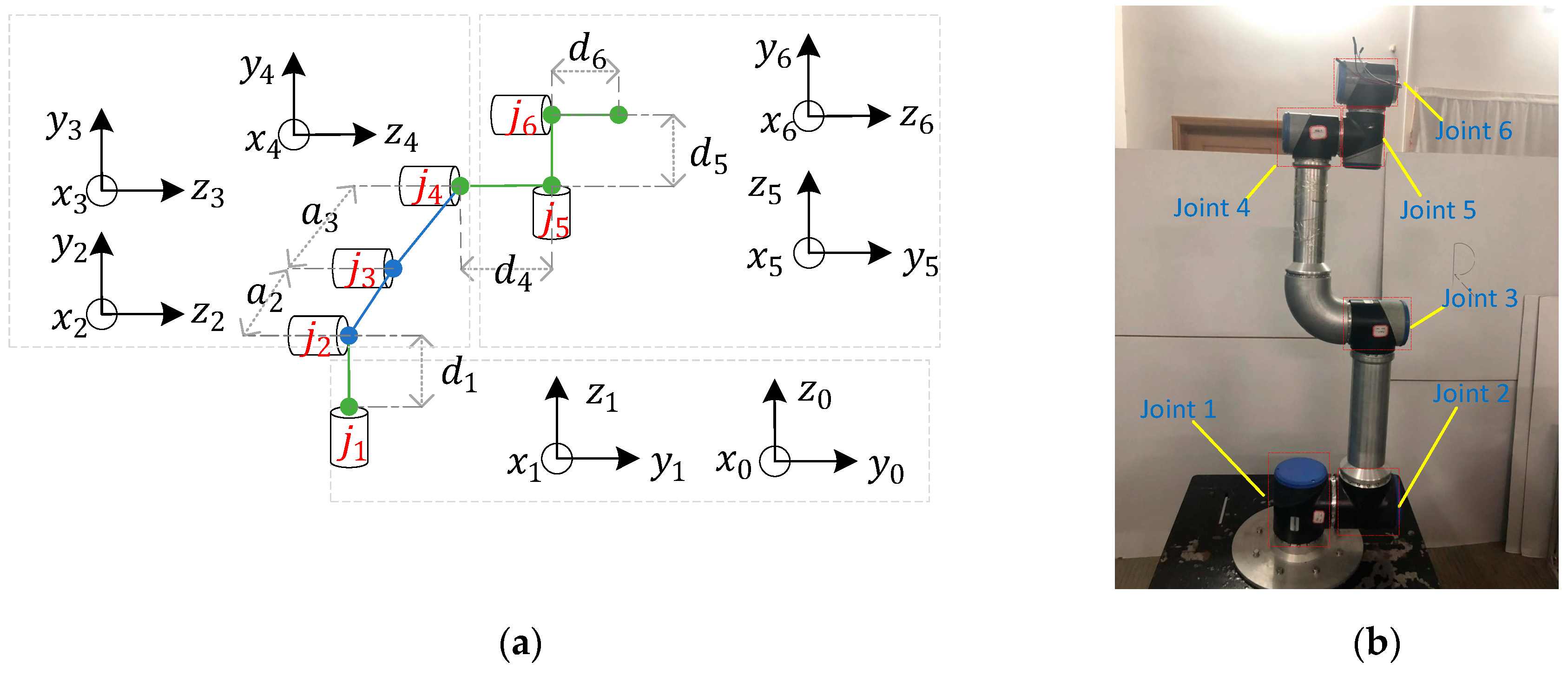
Using the DH method, the relations for a robot can be directly established in a visualized manner and the existence conditions for closed-form solutions can be derived in a more direct and visualized manner. The standard DH parameters in the case of the KingKong collaborative robot are shown in

Table 3. Denavit–Hartenberg (DH) parameters of the KingKong collaborative robot.

n	$\mathit{\theta }$/°	$\mathit{d}$/mm	$\mathit{a}$/mm	$\mathit{\alpha }$/°
1	${\theta }_1$	89.459	0	$\mathsf{\pi }/2$
2	${\theta }_2$	0	−42.5	0
3	${\theta }_3$	0	−39.225	0
4	${\theta }_4$	109.15	0	$\mathsf{\pi }/2$
5	${\theta }_5$	94.65	0	$-\mathsf{\pi }/2$
6	${\theta }_6$	82.3	0	0

. A schematic diagram of the robot is shown in Figure 1.

2.2. Forward Kinematics Formula

Using the following formula, the DH parameters [6] can be transformed into elements of a transformation matrix from [6]:

$${}_k{}^{k-1}T\left({\theta }_i\right)=\left[\begin{array}{cc}{R}_k& P_k\\ 0^{1\times 3}& 1\end{array}\right]=\left[\begin{array}{cccc}cos{\theta }_k& -sin{\theta }_{k}cos{\alpha }_k& sin{\theta }_{k}sin{\alpha }_k& a_{k}cos{\theta }_k\\ sin{\theta }_k& cos{\theta }_{k}cos{\alpha }_k& -cos{\theta }_{k}sin{\alpha }_k& a_{k}sin{\theta }_k\\ 0& sin{\alpha }_k& cos{\alpha }_k& d_k\\ 0& 0& 0& 1\end{array}\right],$$

(1)

where $k$ indicates the number of the current joint. ${}_k{}^{k-1}R$ is the rotational component of ${}_k{}^{k-1}T\left({\theta }_k\right)$, a 3 × 3 orthogonal matrix, and ${}_k{}^{k-1}P$ is the translational component of ${}_k{}^{k-1}T\left({\theta }_k\right)$. The end transformation matrix of the end executor of the robot relative to the coordinate system can be obtained using the following formula:

$${}_i{}^{0}T={}_1{}^{0}T{}_2{}^{1}T{}_3{}^{2}T\cdots {}_i{}^{i-1}T.$$

(2)

$i$ indicates the number of degrees of freedoms of the robot. According to Equation (2) from [18], we could obtain ${}_i{}^{0}T$ as follows:

$${}_i{}^{0}T=\left[\begin{array}{cc}{}_i{}^{0}R& {}_i{}^{0}P\\ 0^{1\times 3}& 1\end{array}\right]=\left[\begin{array}{cc}{\displaystyle \prod _{n=1}^{n=i}}{}_n{}^{n-1}R& {\displaystyle \sum _{n=1}^{n=i}}{}_1{}^{0}R\dots {}_i{}^{i-1}P\\ 0^{1\times 3}& 1\end{array}\right],$$

(3)

where ${}_i{}^{0}R$ is the rotational component of ${}_i{}^{0}T$. Since the rotational component ${}_i{}^{i-1}R$ is closed and orthogonal, ${}_i{}^{0}R$ is an orthogonal matrix. Here, ${}_i{}^{0}P$ is the translational component of ${}_i{}^{0}T$, which can be represented as follows:

$${}_i{}^{0}P={\displaystyle \sum _{n=1}^{n=i}}{}_1{}^{0}R\dots {}_i{}^{i-1}P={\displaystyle \sum _{n=1}^{n=i}}{P}_n.$$

(4)

According to Equation (4), the positional component of the back linkage is influenced by the front joint angle.

In the definition of the DH parameter, the Z-direction of the joint coordinate indicates the orientation of the joint and can be used to characterize the relationship between the joints. Here, the joints of the serial robots are represented as $z_k$. To concisely indicate the linkage relations, the following definitions are made: ${\alpha }_k=0$, then $z_k\parallel z_{k+1}$, whereas ${\alpha }_k=\pm \mathsf{\pi }/2$, then $z_k\perp z_{k+1}$, where $z_k^{a,d}$ represents the linkage parameters $a_k=d_k=0$.

2.3. Decoupling of the End Linkage

The coordinate transformation matrix is written as ${}_{i-1}{}^{0}T=\left[\begin{array}{cc}{}_{i-1}{}^{0}R& {}_{i-1}{}^{0}P\\ 0^{1\times 3}& 1\end{array}\right]$. Moreover, the transformation matrix of the last axis is ${}_i{}^{i-1}T=\left[\begin{array}{cc}{}_i{}^{i-1}R& {}_i{}^{i-1}P\\ 0^{1\times 3}& 1\end{array}\right]$. The rotational component $R$ is written in the form of a row vector as $R=\left[\begin{array}{ccc}\overrightarrow{x}& \overrightarrow{y}& \overrightarrow{z}\end{array}\right]$.

Then, ${}_i{}^{0}P$ can be written as:

$${}_i{}^{0}P={}_{i-1}{}^{0}R\left[\begin{array}{c}cos{\theta }_i\\ sin{\theta }_i\\ 0\end{array}\right]a_i+{}_{i-1}{}^0\overrightarrow{z}{d}_i+{}_{i-1}{}^{0}P,$$

(5)

further:

$${}_{i-1}{}^{0}R\left[\begin{array}{c}cos{\theta }_i\\ sin{\theta }_i\\ 0\end{array}\right]={}_i{}^0\overrightarrow{x}.$$

(6)

The following conclusions can be drawn:

• when ${\alpha }_i=\mathsf{\pi }/2$ then ${}_i{}^0\overrightarrow{y}={}_{i-1}{}^0\overrightarrow{z}$,

  $${}_{i-1}{}^{0}P={}_i{}^{0}P-{}_i{}^0\overrightarrow{x}{a}_i-{}_i{}^0\overrightarrow{y}{d}_i;$$

  (7)
• when ${\alpha }_i=-\mathsf{\pi }/2$ then ${}_i{}^0\overrightarrow{y}=-{}_{i-1}{}^0\overrightarrow{z}$,

  $${}_{i-1}{}^{0}P={}_i{}^{0}P-{}_i{}^0\overrightarrow{x}{a}_i+{}_i{}^0\overrightarrow{y}{d}_i;$$

  (8)
• and when ${\alpha }_i=0$ then, ${}_i{}^0\overrightarrow{z}={}_{i-1}{}^0\overrightarrow{z}$,

  $${}_{i-1}{}^{0}P={}_i{}^{0}P-{}_i{}^0\overrightarrow{x}{a}_i-{}_i{}^0\overrightarrow{z}{d}_i.$$

  (9)

The above derivation demonstrates that when the current end transformation matrix ${}_i{}^{0}T$ is known, the translational component ${}_{i-1}{}^{0}P$ in the previous transformational matrix ${}_{i-1}{}^{0}T$ can be obtained based on the rotational component ${}_i{}^{0}R$ of ${}_i{}^{0}T$ and the translational component ${}_i{}^{0}P$. Given such a property, the last axis may not be considered when the translational component of the robot is being analyzed.

2.4. Translational Relation of the Rotational Component

According to Equation (3) form [6], ${}_k{}^{k-1}R=\mathrm{Rotz}\left({\theta }_k\right)\mathrm{Rotx}\left({\mathsf{\alpha }}_k\right).$ The rotational component of the transformational matrix can be expressed as:

$${}_k{}^{0}R={\prod }_{n=1}^{n=k}{}_n{}^{\mathrm{n}-1}R={\prod }_{n=1}^{n=k}\mathrm{Rotz}\left({\theta }_n\right)\mathrm{Rotx}\left({\mathsf{\alpha }}_n\right).$$

(10)

If there exists several continuous parallel joints in the robot, then $z_l\parallel z_{l+1}\dots \parallel z_m$ and ${\mathsf{\alpha }}_l={\mathsf{\alpha }}_{l+1}\dots ={\mathsf{\alpha }}_{m-1}=0$. In addition, the rotational transformation in the same direction has additivity:

$${}_m{}^{l}R={\displaystyle \prod }_{n=l}^{n=m}\mathrm{Rotz}\left({\theta }_n\right)\mathrm{Rotx}\left({\mathsf{\alpha }}_n\right)=\mathrm{Rotz}\left(\mathsf{\Theta }\right)\mathrm{Rotx}\left({\mathsf{\alpha }}_m\right)=R_{{\theta }_s},$$

(11)

where $\mathsf{\Theta }={\theta }_l+{\theta }_{l+1}\dots +{\theta }_m$. Here, we refer to $z_l\parallel z_{l+1}\dots \parallel z_m$ as a sub-chain $s$. This concept will be used in the following paragraphs. According to Equation (11), the translational components of the sub-chain $z_1\parallel z_2\dots \parallel z_m$ can be defined and simplified as follows:

$${}_m{}^{m-1}P=R_{1.m-1}{P}_m=Rotz\left(\mathsf{\Theta }\right)\left[\begin{array}{c}{a}_m\\ 0\\ 0\end{array}\right]+\left[\begin{array}{c}0\\ 0\\ d_m\end{array}\right]=\left[\begin{array}{c}{a}_m\cos \Theta \\ a_m\sin \Theta \\ d_m\end{array}\right]=P_{{\theta }_s},$$

(12)

where $\mathsf{\Theta }={\theta }_1+{\theta }_2\dots +{\theta }_m$.

$R_{{\theta }_s}$ defined by the formula (11) and $P_{{\theta }_s}$ defined by the formula (12), will be used in the following paragraphs.

2.5. Solving the Trigonometric Equation

This section summarizes two common formula solutions for trigonometric functions. The first can be derived using Equation (4):

$${}_i{}^{0}P={}_1{}^{0}P+{}_1{}^{0}R{\displaystyle \sum _{\mathrm{n}=2}^{n=i}}{}_2{}^{1}R\cdots {}_n{}^{n-1}P=\left[\begin{array}{c}\left({}_i{}^{1}P{}_{y}sin{\alpha }_1-n_1{}_i{}^{1}P{}_x\right)sin{\theta }_1+\left({}_i{}^{1}P{}_z{a}_1+a_1\right)cos{\theta }_1\\ \left({}_i{}^{1}P{}_z{a}_1+a_1\right)sin{\theta }_1-\left(n_1{}_i{}^{1}P{}_y-n_1{}_i{}^{1}P{}_x\right)cos{\theta }_1\\ sin{\alpha }_1{}_i{}^{1}P{}_x+n_1{}_i{}^{1}P{}_y+\left(1+{}_i{}^{1}P{}_z\right)d_1\end{array}\right],$$

(13)

where ${}_i{}^{1}P{}_x,{}_i{}^{1}P{}_y,$ and ${}_i{}^{1}P{}_z$ represent the three components in ${}_1{}^{0}R{}^{-1}\left({}_i{}^{0}P-{}_1{}^{0}P\right)$ and $n_i=sign\left({\alpha }_i\right)$. According to Equation (18), ${}_i{}^{0}P{}_x$, ${}_i{}^{0}P{}_y$, and ${\theta }_1$ satisfy a special trigonometric function relation, as shown in Equation (14):

$$\left[\begin{array}{c}{}_i{}^{0}P{}_x\\ {}_i{}^{0}P{}_y\end{array}\right]=\left[\begin{array}{cc}D& L\\ L& -D\end{array}\right]\left[\begin{array}{c}sin{\theta }_1\\ cos{\theta }_1\end{array}\right],\left(D\ne 0 or L\ne 0\right).$$

(14)

Therefore,

$${\theta }_1=atan2\left(D{}_i{}^{0}P{}_x+L{}_i{}^{0}P{}_y,L{}_i{}^{0}P{}_x-D{}_i{}^{0}P{}_y\right).$$

(15)

Another common trigonometric equation is shown in Equation (16) from [17]:

$$Acos\theta +Bsin\theta =C,\left(A\ne 0 or B\ne 0\right),$$

(16)

whose solution is:

$$\theta =2atan\left(\frac{B\pm \sqrt{B^2+A^2-C^2}}{A+C}\right).$$

(17)

Equations (15) and (17) can map the joint angles within the interval of $[-\mathsf{\pi },\mathsf{\pi }]$. Moreover, in the following paragraphs, the robotic inverse solution equation is transformed into Equations (14) and (16), resulting in a fixed formula, which can compute the equation parameters and further derive the common closed-form formula solution for serial robots. When the parameters for Equations (14) and (16) are zero, the equation has no solution. This provides a suitable answer to the question of whether a robot has a solution when the linkage parameters are sparse. For convenience, Equation (14) is represented as ${\theta }_1=F_1\left(D,L,x,y\right)$ and Equation (15) is represented as ${\theta }_{k1},{\theta }_{k2}=F_2\left(A,B,C\right)$.

3. Analysis of The Inverse Kinematics Problem

Given a transformational matrix with a known end ${}_i{}^{0}T=\left[\begin{array}{cc}{}_i{}^{0}R& {}_i{}^{0}P\\ 0^{1\times 3}& 1\end{array}\right]$, the joint angle is obtained inversely from the equation provided by ${}_i{}^{0}R$ and ${}_i{}^{0}P$; this is known as inverse kinematics.

3.1. Three Types of Sub-Problems Related to Closed-Form Inverse Kinematics

The French mathematician Évariste Galois proved that the quartic polynomial equation has a closed-form solution, whereas the sextic polynomial equation generally has none. The rotational and translational components of the robotic end transformational matrix provide three independent equations separately. The two equation sets are combined to solve the inverse kinematics problem, and then high-order polynomial equations may be required. Therefore, a robot has a closed-form inverse solution, partial joint angles will be preferably solved from a certain equation set followed by the other joint angles.

To guarantee the existence of a closed-form solution, a feasible solution guarantees mutual decoupling between the translational and rotational components [17,26]. Such traditional decoupling enables the translational component to be associated with the front three joints, which in turn, are solved via ${}_3{}^{0}P.$ The latter three joints are solved via the rotational component ${}_6{}^{3}R$.

$${}_6{}^{0}T=\left[\begin{array}{cc}{}_3{}^{0}R& {}_3{}^{0}P\\ 0& 1\end{array}\right]\left[\begin{array}{cc}{}_6{}^{3}R& 0\\ 0& 1\end{array}\right]=\left[\begin{array}{cc}{}_3{}^{0}R{}_6{}^{3}R& {}_3{}^{0}P\\ 0& 1\end{array}\right].$$

(18)

Based on the derivation in Section 2.4, a robot has several parallel joints, the number of unknown numbers in the rotational component will decrease. Therefore, another feasible decoupling idea is to preferably find a solution using the rotational component ${}_6{}^{0}R\left(\mathsf{\phi },\mathsf{\vartheta },\mathsf{\psi }\right)$ and solve for the remaining joint angles using the translational component ${}_6{}^{0}P$. This strategy has not been mentioned in any previous studies.

$${}_6{}^{0}T=\left[\begin{array}{cc}{}_6{}^{0}R& {}_6{}^{0}P\\ 0& 1\end{array}\right]=\left[\begin{array}{cc}{}_6{}^{0}R\left(\mathsf{\phi },\mathsf{\vartheta },\mathsf{\psi }\right)& {}_6{}^{0}P\\ 0& 1\end{array}\right].$$

(19)

Based on the above two decoupling methods, we could obtain three types of sub-problems.

In the first type, when the number of unknowns in the rotational component is larger than three and the robot meets some structural characteristics, some joint angles can be preferably and directly solved using the translational component. This article refers to the first type sub-problem as the sub-problem of translation components.

In the second type, the robot has several parallel joints and the number of unknowns in the rotational component is no greater than 3, these unknowns can be solved using the rotational component. This article refers to the second type sub-problem as sub-problem of rotational components.

In the third and final type, when the second type is used to solve the unknowns for the robot and the joint angles are still not completely solved, the remaining joint angles are obtained using the translational component. This article refers to the third type sub-problem as a sub-problem of sub-chains.

Via an analysis of these sub-problems, it is possible to determine the solving conditions and methods in detail. In Section 3.2, Section 3.3 and Section 3.4, a more detailed analysis and derivation will be made for each sub-problem, and the formulas and conditions for solving the basic problems will be obtained.

3.2. The First Type of Sub-problem

When there exist more than three unknowns in the rotational component, the partial joint angles should preferably be solved using the translational component. With reference to the DH parameter table, the DOF of the robot is $i$ and the number of the DOF with $\mathsf{\alpha }=0$ in the first $i-1$ DOFs is $p$. In the case of $i-p>3$, there are more than three unknowns in the rotational component.

According to Equation (4), the back joint angles are influenced by the front joint angles in the translational component. Therefore, the association with a maximum of the front three joint angles in the translational equation must be first guaranteed to solve the first type of sub-problem.

When the first joint angle of the robot model $Robo{t}_i$ with $i$ DOFs is solved, ${}_1{}^{0}T$ can be calculated using the forward kinematics formula. Meanwhile, the first row of the DH parameters is deleted to form a new robot model $Robo{t}_{i-1}$ and a new transformational matrix ${}_{i-1}{}^{0}T$:

$${}_i{}^{1}T={}_1{}^{0}T{}^{-1}{}_i{}^{0}T=\left[\begin{array}{cc}{}_1{}^{0}R{}^{-1}& -{}_1{}^{0}R{}^{-1}{}_1{}^{0}P\\ 0^{1\times 3}& 1\end{array}\right]{}_i{}^{0}T.$$

(20)

There may only be a parallel or vertical relationship between two adjacent joints. Since only the linkage relation of the front three axes is considered, the possible configuration between the first three axes is only the case where $C_2^1{C}_2^1=4$. Moreover, $z_1\perp z_2\perp z_3$, $z_1\parallel z_2\perp z_3,z_1\perp z_2\parallel z_3\mathrm{and}{z}_1\parallel z_2\parallel z_3$. However, during the process of derivation, it was found that $z_1\parallel z_2\parallel z_3$ only provides two valid equations in X-direction and Y-direction, making it impossible to solve for three unknowns:

$${}_3{}^{0}P=\left[\begin{array}{c}{a}_{3}cos\left({\theta }_1+{\theta }_2+{\theta }_3\right)+a_{2}cos\left({\theta }_1+{\theta }_2\right)+a_{1}cos{\theta }_1\\ a_{3}sin\left({\theta }_1+{\theta }_2+{\theta }_3\right)+a_{2}sin\left({\theta }_1+{\theta }_2\right)+a_{1}sin{\theta }_1\\ d_1+d_2+d_3\end{array}\right].$$

(21)

Such a case is the counter example mentioned in the preceding paragraphs. The Piper principle does not specifically describe such a case. Therefore, the linkage parametric limitations and the formula solution for the three basic problems are derived in detail in the following paragraphs.

3.2.1. First Three Joint Configured as $z_1\parallel z_2\perp z_3^a$

Here, the expression for the translational component is ${}_3{}^{0}P=P_1+R_1{P}_2+R_1{R}_2{P}_3$. However, $R_1{R}_2{P}_3$ contains the cubic term of the sine and cosine functions, which would directly increase the order of the equation to sextic. Only when $a_3=0$ will the requirements for a closed solution be met. According to Equation (18), The formula solution of ${\theta }_1$ can be obtained as follows:

$$\begin{array}{c}{\theta }_{11}=F_1\left(D,L,{}_3{}^{0}P{}_x,{}_3{}^{0}P{}_y\right)\\ {\theta }_{12}=F_1\left(D,-L,{}_3{}^{0}P{}_x,{}_3{}^{0}P{}_y\right)\end{array}, \mathrm{where}\{\begin{array}{c}D=n_1{d}_2\\ L=\sqrt{{}_3{}^{0}P{{}_x}^2+{}_3{}^{0}P{{}_y}^2-D^2}\end{array}.$$

(22)

Once ${\theta }_1$ is obtained, the forward kinematics formula can be used to forward simplify the robot to obtain the expression of ${}_i{}^{1}T$ and the DOFs of $i-1$. The basic problem can still be employed to seek a solution to ${\theta }_2$.

To guarantee the existence of only the front two joint angles in the translational equation, the linkage of $z_{k>3}$ needs to satisfy $d=a=0$. However, according to the end decoupling formula proposed in Section 2.3, the linkage parameters of the last joint are not restricted.

3.2.2. First Three Joint Configured as $z_1\parallel z_2\perp z_3$

The formula solution for $z_1\parallel z_2\perp z_3$ is derived in the following paragraphs. Its translational component can be written as ${}_3{}^{0}P=P_1+P_{12}+R_{12}{P}_3$, and its translational equation can be arranged as follows:

$$\left[\begin{array}{c}{a}_{1}cos{\theta }_1+D\sin \left({\theta }_1+{\theta }_2\right)+L\cos \left({\theta }_1+{\theta }_2\right)\\ a_{1}sin{\theta }_1+L\sin \left({\theta }_1+{\theta }_2\right)-D\cos \left({\theta }_1+{\theta }_2\right)\\ n_2{a}_{3}sin{\theta }_3\end{array}\right]=\left[\begin{array}{c}\begin{array}{c}{}_3{}^{0}P{}_x\\ {}_3{}^{0}P{}_y\end{array}\\ {}_3{}^{0}P{}_z-d_1-d_2\end{array}\right].$$

(23)

Arranging Equation (23) gives the formula solution Equation (24):

$$\begin{array}{c}{\theta }_{31},{\theta }_{32}=F_2\left(A_3,B_3,C_3\right), \mathrm{where}\{\begin{array}{c}{A}_3=0\\ B_3=n_2{a}_3\\ C_3={}_3{}^{0}P{}_z-d_1-d_2\end{array};\\ {\theta }_{11},{\theta }_{12}=F_2\left(A_1,B_1,C_1\right),\mathrm{where}\{\begin{array}{c}{A}_1={}_3{}^{0}P{}_x\\ B_1={}_3{}^{0}P{}_y\\ D=n_2{d}_3\\ L=a_2+a_{3}cos{\theta }_3\\ C_1=\frac{{}_3{}^{0}P{{}_x}^2+{}_3{}^{0}P{{}_y}^2+a_1{}^2-L^2-D^2}{2a_1}\end{array}\\ {\theta }_1+{\theta }_2=F_1\left(\mathrm{D},\mathrm{L},\widetilde{{}_3{}^{0}P{}_x},\widetilde{{}_3{}^{0}P{}_y}\right), \mathrm{where}\{\begin{array}{c}\widetilde{{}_3{}^{0}P{}_x}={}_3{}^{0}P{}_x-a_{1}cos{\theta }_1\\ \widetilde{{}_3{}^{0}P{}_y}={}_3{}^{0}P{}_y-a_{1}sin{\theta }_1\end{array};\\ {\theta }_2=f{\left[\left({\theta }_1+{\theta }_2\right)-{\theta }_1\right]}_{\pm \mathsf{\pi }};\end{array}$$

(24)

where $f{[\theta ]}_{\pm \pi }$ in the last equation indicates that $\theta$ is mapped onto the interval of $[-\mathsf{\pi },\mathsf{\pi }]$.

Under such a structure, ${\theta }_3$ is preferably solved using the equation in the Z-direction. Therefore, the existence of $z_4^a$ after $z_3$ does not influence the solution of ${\theta }_3$, resulting in the derivation of two different structures, $z_1\parallel z_2\perp z_3\perp z_4^a$ and $z_1\parallel z_2\perp z_3\parallel z_4^a$.

According to the translational equation of $z_1\parallel z_2\perp z_3\perp z_4^a$ and Equation (23), the critical coefficient is:

$$\{\begin{array}{l}D=n_2{d}_3+n_2{d}_4\\ L=a_2+a_3\cos {\theta }_3\end{array}.$$

(25)

Moreover, according to Equation (23), the critical coefficient under $z_1\parallel z_2\perp z_3\parallel z_4^a$ is:

$$A_3=-n_2{n}_3{d}_4, \mathrm{where} \{\begin{array}{c}D=n_2{d}_3\\ L=a_2+a_3\cos {\theta }_3+n_3{d}_4\sin {\theta }_3.\end{array}$$

(26)

To guarantee that only the front three joint angles exist in the translational equation, the linkage of $z_{k>4}$ needs to satisfy $d=a=0$. There is not restricted to the linkage parameters of the last joint.

In addition, in the basic problems mentioned above, when $d_4=a_4=0$ is true in $z_4$, it can also be used to solve $z_1\parallel z_2\perp z_3$. Similarly, it can be used to solve $z_1\parallel z_2$. Therefore, such a type of basic problem contains two sets of formula solutions that can be used to solve four cases.

3.2.3. First Three Joint Configured as $z_1\perp z_2\parallel z_3$

The solution method for $z_1\perp z_2\parallel z_3^a$ in Section 3.4.1 also applies here. In addition, if $z_1\perp z_2\parallel z_3\perp z_4^a$ and $D=n_1\left(d_2+d_3\right)$, ${\theta }_1$ can still be directly solved. This results in a special situation. Further, suppose there is a robot with $i$ degrees of freedom, in which the configuration of the first $g$ joints is $z_1\perp z_2\parallel \dots \parallel z_{g-1}\perp z_g^a$, and the linkage of $z_{k>g}$ needs to satisfy $d=a=0$. These are not restricted to the linkage parameters of the last joint. The formula solution of ${\theta }_1$ can be obtained as follows:

$$\begin{array}{c}{\theta }_{11}=F_1\left(D,L,{}_g{}^{0}P{}_x,{}_g{}^{0}P{}_y\right)\\ {\theta }_{12}=F_1\left(D,-L,{}_g{}^{0}P{}_x,{}_g{}^{0}P{}_y\right)\end{array},\mathrm{where} \{\begin{array}{c}D=n_1{\displaystyle \sum _{m=2}^{g-1}}{d}_m\\ L=\pm \sqrt{{}_g{}^{0}P{{}_x}^2+{}_g{}^{0}P{{}_y}^2-D^2}\end{array}.$$

(27)

According to the forward kinematics formula, after ${\theta }_1$ is solved, ${}_1{}^{0}T$ can be cancelled to allow the robot model to reduce a joint angle and become a new model. At that time, selective solving can be performed in all of the sub-problems.

Basic problems 3.2.1 and 3.2.3 can be solved using the same formula solution. In the following paragraphs, basic problem 3.4.1 will be used for the description.

Therefore, there exist two types of basic problems in the first type of sub-problem. This section gives the corresponding relevant existence conditions and formula solutions.

3.3. Solving the Second Type of Sub-Problem

Since the rotational component only provides three independent equations, a maximum of three unknowns can be solved. First, the rotational matrix Rotx($\theta$) is introduced. Rotx($\theta$) represents a $\theta$ radian rotation around the X-coordinate axis. Similarly, Rotz($\theta$) and Roty($\theta$) represent rotations around the Y- and Z-axes. The Euler angle theorem indicates that a generic rotation matrix can be obtained by composing a suitable sequence of three rotations while guaranteeing that two successive rotations are not made around parallel axes [18]. Therefore, any rotational matrix R can be expressed as Rotz($\mathsf{\phi }$), Roty($\mathsf{\vartheta }$), and Rotz($\mathsf{\psi }$).

The DH parameters of a serial robot with a certain DOF are shown in

Table 4. The DH parameters of a serial robot with three degrees-of-freedoms (DOFs).

n	$\mathit{\theta }$/°	$\mathit{d}$/mm	$\mathit{a}$/mm	$\mathit{\alpha }$/°
1	${\theta }_1$	$d_1$	$a_1$	$-\mathsf{\pi }/2$
2	${\theta }_2$	$d_2$	$a_2$	$\mathsf{\pi }/2$
3	${\theta }_3$	$d_3$	$a_3$	0

.

According to the forward kinematics formula,

$$\begin{array}{c}{}_3{}^{0}R=\mathrm{Rotz}\left({\theta }_1\right)\mathrm{Rotx}\left({\mathsf{\alpha }}_1\right)\mathrm{Rotz}\left({\theta }_2\right)\mathrm{Rotx}\left({\mathsf{\alpha }}_2\right)\mathrm{Rotz}\left({\theta }_3\right)\mathrm{Rotx}\left({\mathsf{\alpha }}_3\right),\\ {}_3{}^{0}R=\mathrm{Rotz}\left({\theta }_1\right)\mathrm{Roty}\left({\theta }_2\right)\mathrm{Rotz}\left({\theta }_3\right).\end{array}$$

(28)

A serial robot has three continuous joints meeting ${\alpha }_1=-\frac{\mathsf{\pi }}{2},{\alpha }_2=\frac{\mathsf{\pi }}{2}\mathrm{and}{\alpha }_3=0$, whose rotational components ${}_3{}^{0}R$ are known, two sets of solutions can be found using Euler’s formula.

3.3.1. Three Mutually Perpendicular Sub-Chains

Based on $\alpha$ in the DH parameters, the conclusions in Section 2.4 can be used to simplify the sub-chains and obtain the expression of the rotational matrix,

$${}_3{}^{0}R=\left[\begin{array}{ccc}cos{\theta }_{s_1}cos{\theta }_{s_2}cos{\theta }_{s_3}+n_{s_{1}e}{n}_{s_{2}e}sin{\theta }_{s_1}sin{\theta }_{s_3}& n_{s_{1}e}{n}_{s_{2}e}sin{\theta }_{s_1}cos{\theta }_{s_3}-cos{\theta }_{s_1}cos{\theta }_{s_2}sin{\theta }_{s_3}& n_{s_{2}e}cos{\theta }_{s_1}sin{\theta }_{s_2}\\ sin{\theta }_{s_1}cos{\theta }_{s_2}cos{\theta }_{s_3}-n_{s_{1}e}{n}_{s_{2}e}cos{\theta }_{s_1}sin{\theta }_{s_3}& -n_{s_{1}e}{n}_{s_{2}e}cos{\theta }_{s_1}cos{\theta }_{s_3}-sin{\theta }_{s_1}cos{\theta }_{s_2}sin{\theta }_{s_3}& n_{s_{2}e}sin{\theta }_{s_1}sin{\theta }_{s_2}\\ n_{s_{1}e}sin{\theta }_{s_2}cos{\theta }_{s_3}& -n_{s_{1}e}sin{\theta }_{s_2}sin{\theta }_{s_3}& -n_{s_{1}e}{n}_{s_{2}e}cos{\theta }_{s_2}\end{array}\right],$$

(29)

for which the following expressions can be obtained:

$$\{\begin{array}{c}{\theta }_{s_1}=\mathrm{atan}2\left(n_{s_{2}e}{r}_{23},n_{s_{2}e}{r}_{13}\right)\\ {\theta }_{s_2}=\mathrm{atan}2\left(\sqrt{r_{13}{}^2+r_{23}{}^2},-n_{s_{1}e}{n}_{s_{2}e}{r}_{33}\right)\\ {\theta }_{s_3}=\mathrm{atan}2\left(-n_{s_{1}e}{r}_{32},n_{s_{1}e}{r}_{31}\right)\end{array},$$

(30a)

or

$$\{\begin{array}{c}{\theta }_{s_1}=\mathrm{atan}2\left(-n_{s_{2}e}{r}_{23},-n_{s_{2}e}{r}_{13}\right)\\ {\theta }_{s_2}=\mathrm{atan}2\left(-\sqrt{r_{13}{}^2+r_{23}{}^2},-n_{s_{1}e}{n}_{s_{2}e}{r}_{33}\right)\\ {\theta }_{s_3}=\mathrm{atan}2\left(n_{s_{1}e}{r}_{32},-n_{s_{1}e}{r}_{31}\right)\end{array},$$

(30b)

where ${\theta }_{s_k}$ represents the sum of the rotation angles of the $k$th sub-chain of the robot and $n_{s_{k}e}$ represents the symbol of the last linkage $\alpha$ in the $k\mathrm{th}$ sub-chain. $r_{xy}$ represents the element at the position of the $x$th row and the $y$th column of the rotation matrix ${}_3{}^{0}R$. The problem of solving the sum of the rotation angles of three mutually perpendicular sub-chains is referred to as basic problem 3.3.1.

3.3.2. Two Mutually Perpendicular Sub-Chains

Similarly, when there are only two mutually perpendicular sub-chains, the expression of the rotational component at that time is as follows:

$${}_2{}^{0}R=\left[\begin{array}{ccc}cos{\theta }_{s_1}cos{\theta }_{s_2}& -cos{\theta }_{s_1}sin{\theta }_{s_2}& n_{s_{1}e}sin{\theta }_{s_1}\\ sin{\theta }_{s_1}cos{\theta }_{s_2}& -sin{\theta }_{s_1}sin{\theta }_{s_2}& -n_{s_{1}e}cos{\theta }_{s_1}\\ n_{s_{1}e}sin{\theta }_{s_2}& n_{s_{1}e}cos{\theta }_{s_2}& 0\end{array}\right],$$

(31)

with the corresponding solution:

$$\{\begin{array}{c}{\theta }_{s_2}=\mathrm{atan}2\left(n_{s_{1}e}{r}_{31},n_{s_{1}e}{r}_{33}\right)\\ {\theta }_{s_1}=\mathrm{atan}2\left(\frac{r_{21}}{cos{\theta }_{s_2}},\frac{r_{11}}{cos{\theta }_{s_2}}\right)\end{array}.$$

(32)

$r_{xy}$ represents the element at the position of the $x$th row and the $y$th column of the rotation matrix ${}_2{}^{0}R$. The problem of solving the sum of the rotational degrees of two mutually perpendicular sub-chains is referred to as basic problem 3.3.2.

3.4. The Third Type of Sub-Problem

Before the second type of sub-problem is employed by the governing algorithm, the DOF of the robot at that time is $i$, then the number of DOFs with $\mathsf{\alpha }=0$ in the first $i-1$ DOFs is $p$. If $p\ne 0$, not all joint angles are obtained by the second type of sub-problem. In this case, the translational component needs to be employed to solve for the remaining joint angles. Such problems are called the third type of sub-problem.

For any of this type of sub-problem, when the first chain only has one joint, the forward kinematics formula can be directly used to simplify the robotic model. Based on that and according to Equation (4), the translational components of a robot with a DOF of $i$ can be divided into $i$ components. Since the second type of sub-problem can solve the sum of the rotational angles of the sub-chains of the robot, based on Equation (17), the translational equation can be arranged as

$${}_i{}^{0}P-P_{{\theta }_{s_1}}-R_{{\theta }_{s_1}}{P}_{{\theta }_{s_2}}-R_{{\theta }_{s_1}}{R}_{{\theta }_{s_2}}{P}_{{\theta }_{s_3}}={\sum }_{n=1}^{n=i}{}_n{}^{n-1}P-P_{{\theta }_{s_1}}-R_{{\theta }_{s_1}}{P}_{{\theta }_{s_2}}-R_{{\theta }_{s_1}}{R}_{{\theta }_{s_2}}{P}_{{\theta }_{s_3}}.$$

(33)

$P_{{\theta }_{s_k}}$ and $P_{{\theta }_{s_k}}$ represent the rotational and translational components of the $k$th sub-chain, which is defined by the formula (11) and formula (12). All terms on the left side of Equation (33) are known and are written as $\widehat{P}$ in the following paragraphs. Conversely, there are unknown quantities on the right side of the equation. Since the third type of problem has a maximum of three sections of sub-chains, $\left[s_1,s_2,s_3\right]$ is used to represent the length of each sub-chain on the right side of the equation. Depending on the length of each sub-chain, the appropriate formula solutions are presented with $s_{i}t$ representing the $t$th joint in the $i$th section of the sub-chain.

As an example, for $z_1\parallel z_2\perp z_3\parallel z_4$, there exist two sub-chains, $s_1\mathrm{and}{s}_2$, either of which has a sub-chain length of two. After the second type of sub-problem is solved, the length of each sub-chain decreases by one. For example, the length of each sub-chain on the right side of Equation (33) is $[1,1,0]$.

All possible cases will be analyzed and solved for in the following cases.

3.4.1. Sub-Chain Length as [1,0,0]

$$\begin{array}{c}{\theta }_{s_{1}1}=atan2\left(a_{s_{1}1}{\widehat{P}}_y,a_{s_{1}1}{\widehat{P}}_x\right).\\ {\theta }_{s_{1}2}={\left[{\theta }_{s_1}-{\theta }_{s_{1}1}\right]}_{\pm \mathsf{\pi }}.\end{array}$$

(34)

3.4.2. Sub-Chain Length as [2,0,0]

$$\begin{array}{c}{\theta }_{s_{1}11},{\theta }_{s_{1}12}=F_2\left(\mathrm{A},\mathrm{B},\mathrm{C}\right), \mathrm{where} \{\begin{array}{c}A={\widehat{P}}_x\\ B={\widehat{P}}_y\\ C=\frac{{\widehat{P}}_x{}^2+{\widehat{P}}_y{}^2+a_{s_{1}1}{}^2-a_{s_{1}2}{}^2}{2a_{s_{1}1}}\end{array}.\\ {\theta }_{s_{1}1}+{\theta }_{s_{1}2}=F_1\left(\mathrm{D},\mathrm{L},\widetilde{P_x},\widetilde{P_y}\right), \mathrm{where} \{\begin{array}{c}\widetilde{P_x}={\widehat{P}}_x-a_{s_{1}1}\cos {\theta }_{s_{1}1}\\ \widetilde{P_y}={\widehat{P}}_y-a_{s_{1}1}\sin {\theta }_{s_{1}1}\\ L=a_{s_{1}2}\\ D=0\end{array}\\ {\theta }_{s_{1}2}=f{\left[\left({\theta }_{s_{1}1}+{\theta }_{s_{1}2}\right)-{\theta }_{s_{1}1}\right]}_{\pm \mathsf{\pi }}\\ {\theta }_{s_{1}3}=f{\left[{\theta }_{s_1}-\left({\theta }_{s_{1}1}+{\theta }_{s_{1}2}\right)\right]}_{\pm \mathsf{\pi }}\end{array}$$

(35)

3.4.3. Sub-Chain Length as [2,1,0] and [1,1,0]

$${\theta }_{s_{2}11},{\theta }_{s_{2}12}=F_2\left(A,\mathrm{B},\mathrm{C}\right), \mathrm{where} \{\begin{array}{c}A=0\\ B=n_{s_{1}e}{a}_{s_{2}1}\\ C={\widehat{P}}_z-d_{s_{1}1}-d_{s_{1}2}\end{array}.$$

(36a)

$${\theta }_{s_{2}2}=f{\left[{\theta }_{s_1}-{\theta }_{s_{1}1}\right]}_{\pm \mathsf{\pi }}.$$

(36b)

$$\widehat{P}-R_{s_1}{P}_{s_{2}1}=P_{s_{1}1}+R_{s_{k}1}{P}_{s_{k}2}.$$

(36c)

$R_{s_{k}t}$ and $P_{s_{k}t}$ represent the rotational and translational components of the $t$th joint in the $k$th section of the sub-chain. According to Equations (36a) and (36b), all joint angles in the sub-chain $s_2$ can be solved. Moreover, according to Equation (36c), the first sub-chain solving problem is transformed into either basic problem 3.6.1 or basic problem 3.6.2.

3.4.4. Sub-Chain Length as [1,2,0]

$${\theta }_{s_{1}11},{\theta }_{s_{1}12}=F_2\left(A,\mathrm{B},\mathrm{C}\right),\mathrm{where}\{\begin{array}{c}A=n_{s_{1}2}{a}_{s_{1}2}\sin {\theta }_{s_1}\\ B=-n_{s_{1}2}{a}_{s_{2}1}\sin {\theta }_{s_1}\\ C={\left(R_{s_1}{}^T \widehat{P}\right)}_z-d_{s_{2}1}-d_{s_{2}2}\end{array}.$$

(37a)

$${\theta }_{s_{1}2}=f{\left[{\theta }_{s_1}-{\theta }_{s_{1}1}\right]}_{\pm \mathsf{\pi }}.$$

(37b)

$$R_{s_1}{}^T\left(\widehat{P}-P_{s_{1}1}\right)=P_{s_{2}1}+R_{s_{2}1}{P}_{s_{2}2}.$$

(37c)

According to Equations (37a) and (37b), we could solve all joint angles in the sub-chain $s_1$. According to Equation (37c), the second sub-chain solving problem can be transformed into basic problem 3.4.2.

3.4.5. Sub-Chain Length as [2,0,1] or [1,0,1]

$${\theta }_{s_{3}11},{\theta }_{s_{3}12}=F_2\left(A,B,C\right),\mathrm{where}\{\begin{array}{c}A=0\\ B=n_{s_{1}e}{a}_{s_{3}1}sin{\theta }_{s_3}\\ C={\widehat{P}}_z-d_{s_{1}1}-d_{s_{1}2}+n_{s_{1}3}{n}_{s_{2}1}{d}_{s_{3}1}cos{\theta }_{s_3}\end{array}.$$

(38a)

$${\theta }_{s_{3}2}=f{\left[{\theta }_{s_3}-{\theta }_{s_{3}1}\right]}_{\pm \mathsf{\pi }}.$$

(38b)

$$\widehat{P}-R_{s_1}{R}_{s_2}{P}_{s_{3}2}=P_{s_{2}1}+R_{s_{2}1}{P}_{s_{2}2}.$$

(38c)

According to Equations (38a) and (38b), all joint angles in the sub-chain $s_3$ can be solved. According to Equation (38c), the first sub-chain solving problem can be transformed into either basic problem 3.4.2 or basic problem 3.4.1.

3.4.6. Sub-Chain Length as [1,0,2]

$${\theta }_{s_{1}21},{\theta }_{s_{1}22}=F_2\left(A,\mathrm{B},\mathrm{C}\right),\mathrm{where}\{\begin{array}{c}A=0\\ B=n_{s_{2}1}{a}_{s_{1}1}sin{\theta }_{s_2}\\ C={(R_{s_2}{}^T{R}_{s_1}{}^T\widehat{P})}_z-d_{s_{3}1}-d_{s_{3}2}+n_{s_{1}2}{n}_{s_{2}1}{d}_{s_{1}1}cos{\theta }_{s_2}\end{array}.$$

(39a)

$${\theta }_{s_{1}1}=f{\left[{\theta }_{s_1}-{\theta }_{s_{1}2}\right]}_{\pm \mathsf{\pi }}.$$

(39b)

$$R_{s_2}{}^T{R}_{s_1}{}^T\widehat{P}-R_{s_2}{}^T{R}_{s_1}{}^T{P}_{s_{1}1}=P_{s_{3}1}+R_{s_{3}1}{P}_{s_{3}2}.$$

(39c)

According to Equations (39a) and (39b), we could solve all joint angles in the sub-chain $s_1$. According to Equation (39c), the third sub-chain solving problem can be transformed into basic problem 3.4.2.

In the case of [1,1,1], it may be impossible to find a closed-form solution due to the high complexity of the equation. Therefore, the third type of sub-problem has six basic problems.

3.5. Summary

The above-mentioned content proposed the two decoupling methods of series robots firstly. Three types of sub-problems are proposed through these two decoupling methods. Ten basic problems were derived through analyzing the solvable condition and solution method of each type of sub-problems specifically. If a series robot can be described through the three types of sub-problem based on these ten basic problems, the robot must be a closed inverse solution.

$\mathrm{P}$ represents the number of the DOF with $\mathsf{\alpha }=0$ in the first $i-1$ DOFs, i.e., the number of $\mathsf{\alpha }=0$ in the first $i-1$ rows of the DH parameter table.

In the case of $i-P>3$, it means that there are more vertical joints in the robot. There will be more than three unknown numbers that cannot be solved in the rotational component. If there is a closed solution, a low-order trigonometric function equation can only be solved through translation components. There are two basic problems that are feasible. The restrictions and solution formula of the two basic problems is shown in

Table 5. The restrictions and solution formula of the two basic problems.

Base Problem	Configuration Restrict	Solution Formula
3.2.1	1. The configuration of the first g joints is $z_1\perp z_2\parallel \dots \parallel z_{g-1}\perp z_g^a,$ 2. The linkage of $z_{k>g}$ needs to satisfy $d=a=0.$. 3. The linkage parameters of the last joint are not restricted.	Equation (30) can be used to solve ${\theta }_1$
3.2.2	1. The configuration of the first three joints is $z_1\parallel z_2\perp z_3,$ 2. The linkage of $z_{k>4}$ needs to satisfy $d=a=0$. 3. The linkage parameters of the last joint are not restricted.	Equations (25) and (26) can be used to solve critical coefficient, formula (24) can be used to solve the angle of first three joints.

.

In the case of $i-P<3$, it means that there are more parallel joints in the robot. There will be less than three unknown numbers in the rotational component, then, the unknown number can be solved through in the rotational component directly. The parallel joints in the rotation component may be an independent joint angle or the sum of the rotation angles of the sub-chains; therefore, they can be represented as unknown number here. In the case of $i-P=3$, the formula (30) can be used to solve the three-unknown number. In the case of $i-P=2$, the formula (32) can be used to solve the two-unknown number. In the case of $i-P=1$, the first formula in the formula (32) can be used to solve the only unknown number.

If all joint angles are not solved after using the second sub-problems, it indicates that there is long sub-chain in the translational component. At this time, the remaining joint angles need to be solved by combing the third sub-problems with the result of the second sub-problems. The six basic problems in the third sub-problems are shown in

Table 6. The six basic problems in the third sub-problems.

Base problem	Remaining Length of Each Sub-Chain	Solution Formula
3.4.1	[1,0,0]	Equation (34)
3.4.2	[2,0,0]	Equation (35)
3.4.3	[2,1,0], [1,1,0]	Equation (36) and Base problem 3.6.2.
3.4.4	[1,2,0]	Equation (37) and Base problem 3.6.2.
3.4.5	[2,0,1], [1,0,1]	Equation (38) and Base problem 3.6.2 or 3.6.1.
3.4.6	[1,0,2]	Equation (39) and Base problem 3.6.2.

.

Since the third type of problem has a maximum of three sections of sub-chains, $\left[s_1,s_2,s_3\right]$ is used to represent the length of each sub-chain on the right side of the equation. Depending on the length of each sub-chain, the appropriate formula solutions are presented with $s_{k}t$ representing the $t$th joint in the $k$th section of the sub-chain.

4. Algorithm Design for Universal Inverse Kinematics

The translational and rotational components of a serial robot with a closed-form solution are mutually decoupled. Therefore, the partial joint angles of the robot can be solved based on the first or second type of sub-problem. This simplifies the original robot model into a new robot model. If the new robot model has a closed-form solution, the solution will definitely continue along one of the three types of sub-problems until all the problems are solved. Therefore, the process of solving the closed-form inverse solution of a serial robot can be completed via constant model simplification. The logical flow chart of the entire algorithm is shown in Figure 2.

In Figure 2, $\mathrm{P}$ represents the number of the DOF with $\mathsf{\alpha }=0$ in the first $i-1$ DOFs, i.e., the number of $\mathsf{\alpha }=0$ in the first $i-1$ rows of the DH parameter table.

The inverse kinematics problem has multiple solutions. Nonetheless, the selection of these solutions necessitates a relevant upper logic design. In addition, changes in the robotic joints must be continuous:

$$arg {\displaystyle \underset{k}{min}}{\displaystyle \sum _{i=1}^6}\left|{\theta }_{i,cur}-{\theta }_{i,k}\right|.$$

(40)

In cases where the robot is in a stationary state, the joint angle of the $k$ set can be first solved and then Equation (40) can be used to determine the inverse motion index value corresponding to the current position.

The main purpose of this paper was to find a more complete inverse solution judgment condition, which is more accurate and specific than the Pieper principle. The general inverse solution algorithm designed based on this judgment condition is also directed to a series robot with a closed inverse solution. For this paper purposed ten basic problems, which means a series of robots with closed inverse solutions can be obtained through combining the basic problems. For example, although $z_1\parallel z_2\perp z_3\parallel z_4^a\perp z_5^{a,d}\perp z_6$, or $z_1\parallel z_2\perp z_3\parallel z_4\parallel z_5\parallel z_6$ are not common, but it is indeed that there are robots with a closed inverse solution. In addition, maintaining the robot configuration does not change, only the direction of rotation and the positive or negative of the offset are changed, the algorithm can still calculate correctly. This can provide great convenience for the application of an engineer. Finally, the logical design of the algorithm is complete. This means that once you use a situation other than ten basic questions to design the robot, the algorithm will jump out and terminate. Therefore, the algorithm is not to solve the inverse solution problem of any robot, but to judge whether the closed inverse solution exists and to solve it.

5. Experiments

The previous section discussed the design of the universal inverse kinematics solution algorithm. In this section, four of the experiments will be carried out to verify the completeness, versatility, stability, and real-time performance of the algorithm.

Frist of all, the algorithm was implemented in MATLAB 2016b on a 64-bit Windows 10 operating system. The completeness, versatility and stability of the algorithm will be verified in MATLAB. Subsequently, the algorithm was performed using the Beckhoff-C6920 controller. We built a six-DOF KingKong robot using the Kollmorgen RGM motor for the real-time testing.

5.1. Verification Experiment for Algorithm Completeness

Firstly, the algorithm designed in this paper was logically complete. The first simulation experiment would test the completeness of the algorithm. Here, a robot with three parallel joints was selected as the experimental object. The DH parameter of it is shown in the

Table 7. The DH parameters of the robot with three parallel joints.

n	$\mathit{\theta }$/°	$\mathit{d}$/mm	$\mathit{a}$/mm	$\mathit{\alpha }$/°
1	${\theta }_1$	0.1	0.1	0
2	${\theta }_2$	0.1	−0.2	0
3	${\theta }_3$	0.1	0.3	0

. This robot is a common series robot, but it cannot be described by a single sub-problem.

First, the algorithm receives the DH parameters of the robot. Algorithm will enter in the second type of sub-problem to solve the rotation angle and ${\theta }_{s_1}$ of the sub-chain $s_1$. The length of the sub-chain was $[2,0,0]$ after been simplified and calculated, therefore, the remaining joint angles was solved by the basic problem 3.6.2 in the third type sub-problems.

Consequently, the initial position was $\mathsf{\Theta }=\left[\begin{array}{c}90°\\ 90°\\ 45°\end{array}\right]$, and the end posture was:

$$\left[\begin{array}{cccc}-0.7071& 0.7071& 0& -0.0121\\ -0.7071& -0.7071& 0& -0.1121\\ 0& 0& 1& 0.3\\ 0& 0& 0& 1\end{array}\right].$$

(41)

All joint angles were solved with the algorithm, as shown in

Table 8. Two inversely solved joint angle sets.

No.	${\mathit{\theta }}_1$/°	${\mathit{\theta }}_2$/°	${\mathit{\theta }}_3$/°
1	90	90	45
2	−36.8699	−90	−8.1301

.

It is easy to verify that the two sets of joint angles are correct.

A robot with four parallel joints was now used as the experimental object. Its DH parameters are shown in

Table 9. The DH parameters of the robot with three parallel joints.

n	$\mathit{\theta }$/°	$\mathit{d}$/m	$\mathit{a}$/m	$\mathit{\alpha }$/°
1	${\theta }_1$	0.1	0.1	0
2	${\theta }_2$	0.1	−0.2	0
3	${\theta }_3$	0.1	0.3	0
4	${\theta }_4$	0.1	0.1	0

.

The algorithm will enter in the second type of sub-problem the solve the rotation angle and ${\theta }_{s_1}$ of the sub-chain $s_1$. The length of the sub-chain was [3,0,0] after being simplified and calculated, the algorithm was ended for it was not in the basic problem of the third type sub-problems. In fact, there are only three valid equations for series robots with four-degree-of-freedom, which is impossible to solve its inverse motion problem.

Experiment 5.1 verified the completeness of the algorithm by two examples. The first example was a three-parallel joint robot, the correct joint angles were obtained through an algorithm. Then, we used a four-parallel joint robot to test, and the algorithm was terminated for it was not in the basic problems. This shows that the algorithm would exit correctly when it encounters an unsolvable problem, and it will be able to calculate the result when it encounters a solvable problem.

This experiment also proved that the proposed judgment method could be used to low-degree-of-freedom robots. In addition, when there were four adjacent parallel joints in a six-degree-of-freedom robot, the Pieper criterion was satisfied, but the proposed algorithm could judge that the robot did not have a closed inverse solution. This complements the shortcomings of the Pieper criterion.

5.2. Verification Experiment of Algorithm Versatility

The proposed algorithm could solve those serial robots that could be described by three types of sub-problems. Since the description of the ten basic problems was determined, a series robot with a closed-form inverse solution could be constructed based on ten basic problems. Two uncommon robots were used as examples to verify the versatility of the algorithm in this experiment.

We constructed a robot $Bo{t}_1$, whose structure was $z_1\parallel z_2\perp z_3\parallel z_4^a\perp z_5^{a,d}\perp z_6$ based on basic problem 3.4.2 and 3.5.1. Its DH parameters are shown in

Table 10. The DH parameters of $Bo{t}_1$.

n	$\mathit{\theta }$/°	$\mathit{d}$/m	$\mathit{a}$/m	$\mathit{\alpha }$/°
1	${\theta }_1$	0.1	0.35	0
2	${\theta }_2$	0.1	0.3	$\mathsf{\pi }/2$
3	${\theta }_3$	0.1	0.5	0
4	${\theta }_4$	0.1	0	$-\mathsf{\pi }/2$
5	${\theta }_5$	0	0	$\mathsf{\pi }/2$
6	${\theta }_6$	0.1	0.1	0

.

The robot had three vertical joints, so the decoupling of the end was carried out firstly. Then, we found that $z_1\parallel z_2\perp z_3\parallel z_4^a\perp z_5^{a,d}$ could be solved by the basic problem 3.2.2. When the first three joint angles were solved, the simplified robot $z_4^a\perp z_5^{a,d}\perp z_6$ could be solved by the second type of sub-problems.

Consequently, the initial position was $\mathsf{\Theta }=\left[\begin{array}{c}90°\\ 60°\\ 60°\\ 60°\\ 30°\\ 30°\end{array}\right]$, and the end posture was:

$$\left[\begin{array}{cccc}0.5625& 0.1752& 0.8080& -0.0228\\ -0.8248& 0.1875& 0.5335& 0.6441\\ -0.0580& -0.9665& 0.2500& 0.7192\\ 0& 0& 0& 1\end{array}\right].$$

(42)

All joint angles were solved with an algorithm, as shown in

Table 11. Four inversely solved joint angle sets.

No.	${\mathit{\theta }}_1$/°	${\mathit{\theta }}_2$/°	${\mathit{\theta }}_3$/°	${\mathit{\theta }}_4$/°	${\mathit{\theta }}_5$/°	${\mathit{\theta }}_6$/°
1	90.0000	60.0000	90.0000	−120.0000	−30.0000	−150.0000
2	90.0000	60.0000	90.0000	60.0000	30.0000	30.0000
3	116.7078	7.3801	90.0000	−177.4728	−14.4919	−89.1752
4	116.7078	7.3801	90.0000	2.5272	14.4919	90.8248

.

It is easy to verify that the four sets of joint angles are correct. Then, we kept the configuration of the robot unchanged and modified the positive direction of the rotation of the robot joint, the positive and negative of $a$ and the value of $d$. This was used to verify whether the algorithm could cope with parameter changes. The changed DH parameters are shown in

Table 12. The DH parameters of $Bo{t}_1$ after changing the parameters.

n	$\mathit{\theta }$/°	$\mathit{d}$/m	$\mathit{a}$/m	$\mathit{\alpha }$/°
1	${\theta }_1$	0	−0.35	0
2	${\theta }_2$	0	0.3	$\mathsf{\pi }/2$
3	${\theta }_3$	0	−0.5	0
4	${\theta }_4$	0	0	$\mathsf{\pi }/2$
5	${\theta }_5$	0	0	$\mathsf{\pi }/2$
6	${\theta }_6$	0	0.1	0

.

Consequently, the initial position was $\mathsf{\Theta }=\left[\begin{array}{c}90°\\ 60°\\ 60°\\ 60°\\ 30°\\ 30°\end{array}\right]$, and the end posture was:

$$\left[\begin{array}{cccc}0.5625& -0.8248& 0.0580& -0.2036\\ 0.1752& 0.1875& 0.9665& -0.1825\\ -0.8080& -0.5335& 0.2500& 0.4192\\ 0& 0& 0& 1\end{array}\right].$$

(43)

All joint angles were computed with the algorithm, as shown in

Table 13. Four inversely solved joint angle sets.

No.	${\mathit{\theta }}_1$/°	${\mathit{\theta }}_2$/°	${\mathit{\theta }}_3$/°	${\mathit{\theta }}_4$/°	${\mathit{\theta }}_5$/°	${\mathit{\theta }}_6$/°
1	90.0000	60.0000	90.0000	−120.0000	−30.0000	−150.0000
2	90.0000	60.0000	90.0000	60.0000	30.0000	30.0000
3	−14.8218	−60.0000	90.0000	105.2403	−108.0015	51.7522
4	−14.8218	−60.0000	90.0000	−74.7597	108.0015	–128.2478

It is easy to verify that the four sets of joint angles are correct.

We constructed the robot $Bo{t}_2$, whose structure was $z_1\parallel z_2\perp z_3\parallel z_4\parallel z_5\parallel z_6$ based on basic problem 3.5.1 and 3.6.6. Its DH parameters are shown in

Table 14. The DH parameters of $Bo{t}_2$.

n	$\mathit{\theta }$/°	$\mathit{d}$/m	$\mathit{a}$/m	$\mathit{\alpha }$/°
1	${\theta }_1$	0.1	0.35	0
2	${\theta }_2$	0.1	0.3	$-\mathsf{\pi }/2$
3	${\theta }_3$	0.1	0.3	$\mathsf{\pi }/2$
4	${\theta }_4$	0.1	0.25	0
5	${\theta }_5$	0.1	0.2	0
6	${\theta }_6$	0.1	0.1	0

.

The robot had three sub-chains, and the second type of sub-problem was firstly used to obtain the sum of the rotation angle of the three segments. Then, algorithm turned into the third type sub-problems for there were joint angles that had not been solved. In the third sub-problem, we could use the basic problem 3.6.6 to solve, and then solve all joint angles.

Consequently, the initial position was $\mathsf{\Theta }=\left[\begin{array}{c}90°\\ 60°\\ 60°\\ 45°\\ 45°\\ 45°\end{array}\right]$, and the end posture was:

$$\left[\begin{array}{cccc}-0.0474& 0.6597& -0.7500& -0.9344\\ -0.7891& 0.4356& 0.4330& 0.2573\\ 0.6124& 0.6124& 0.5000& -0.0017\\ 0& 0& 0& 1\end{array}\right].$$

(44)

All joint angles were solved with the algorithm, as shown in

Table 15. Four inversely solved joint angle sets.

No.	${\mathit{\theta }}_1$/°	${\mathit{\theta }}_2$/°	${\mathit{\theta }}_3$/°	${\mathit{\theta }}_4$/°	${\mathit{\theta }}_5$/°	${\mathit{\theta }}_6$/°
1	−150.0000	−60.0000	60.0000	−95.1093	100.7234	129.3859
2	−150.0000	−60.0000	60.0000	−9.6646	−100.7234	−114.6120
3	90.0000	60.0000	60.0000	45.0000	45.0000	45.0000
4	90.0000	60.0000	60.0000	84.7298	−45.0000	95.2702

.

It is easy to verify that the four sets of joint angles are correct.

In this group of experiments, the test subjects were two uncommon robots constructed by basic questions. However, according to the proposed theory, these two robots had a closed inverse solution. In the experiment, the inverse solution of both robots was solved correctly. In addition, for the first robot, its configuration remains unchanged, but the link parameters were greatly modified, the correct result was obtained in the end. It could be seen that the algorithm had good versatility. As long as a given robot can be described by three sub-problems, its closed-from solution can be obtained whether it is in low degree of freedom or six degrees of freedom. At the same time, for the robot with the same configuration, the change of the link parameters does not affect the inverse kinematics solution.

5.3. Verification Experiment for the Algorithm Continuity

This experiment would use the common Puma560 as the subject. In the experiment, the robot should move according to the specified trajectory. We needed to observe whether the joint angle after the inverse solution was continuous when solving the continuous space trajectory. This is important in the actual movement of robot. If there is a jump or discontinuity in the joint space curve, it will cause great impact to the motor, and the curve of the end also does not move according to the specified trajectory. The DH parameters of the Puma560 robot are shown in

Table 16. The DH parameters of the Puma560 robot.

n	$\mathit{\theta }$/°	$\mathit{d}$/mm	$\mathit{a}$/mm	$\mathit{\alpha }$/°
$1$	${\theta }_1$	0	0	$\mathsf{\pi }/2$
$2$	${\theta }_2$	0	43.18	0
$3$	${\theta }_3$	150.03	20.3	$-\mathsf{\pi }/2$
$4$	${\theta }_4$	43.18	0	$\mathsf{\pi }/2$
$5$	${\theta }_5$	0	0	$-\mathsf{\pi }/2$
$6$	${\theta }_6$	0	0	0

.

The quantity of the vertical joints was judged following the input of the algorithm into the DH model of the Puma560 robot. Subsequently, the algorithm entered the first type of sub-problem. Then, joint decoupling was performed for $J_6$ and $J_1\perp J_2\parallel J_3\perp J_{4,a}\perp J_{5,a,d}$. Based on basic problem 3.4.1, the angle value of ${\theta }_1$ was obtained. In addition, after ${\theta }_1$ was obtained, ${}_6{}^{1}T$ was obtained using to the forward kinematics formula. After it was simplified, $J_2\parallel J_3\perp J_{4,a}\perp J_{5,a,d}\perp J_6$ formed a new robot model and was substituted into the algorithm. Similarly, $J_2\parallel J_3\perp J_{4,a}\perp J_{5,a,d}$ was solved using basic problem 3.2.2 and ${\theta }_2\mathrm{and}{\theta }_3$ were subsequently obtained. After the reduction in the DH parameters and the transformational matrices, ${}_6{}^{4}T$ and the robot model $J_{4,a}\perp J_{5,a,d}\perp J_6$ were substituted into the algorithm to solve the rational component in the second type of sub-problem. All joint angles were solved at that time.

Consequently, the initial position was $\mathsf{\Theta }=\left[\begin{array}{c}25.5667°\\ -0.0624°\\ 3.0736°\\ -25.5975°\\ 87.2840°\\ 1.3005°\end{array}\right]$, and the end execution posture was:

$$\left[\begin{array}{cccc}0& 0& -1& 0.4521\\ 0& 1& 0& 0.0499\\ 1& 0& 0& 0.4318\\ 0& 0& 0& 1\end{array}\right].$$

(45)

All joint angles were computed with the algorithm, as shown in

Table 17. Eight inversely solved joint angle sets.

No.	${\mathit{\theta }}_1$/°	${\mathit{\theta }}_2$/°	${\mathit{\theta }}_3$/°	${\mathit{\theta }}_4$/°	${\mathit{\theta }}_5$/°	${\mathit{\theta }}_6$/°
1	167.0434	89.6199	3.0711	−78.4733	166.7756	101.8339
2	167.0434	89.6199	3.0711	101.5267	−166.7756	−78.1661
3	167.0434	−179.9370	−177.6878	167.0362	92.3124	0.5341
4	167.0434	−179.9370	−177.6878	12.9638	−92.3124	−179.4659
5	25.5654	−0.0630	3.0711	−25.5998	87.2844	1.3006
6	25.5654	−0.0630	3.0711	154.4002	−87.2844	178.6994
7	25.5654	90.3801	−177.6878	−84.3875	154.2989	−83.7756
8	25.5654	90.3801	−177.6878	95.6125	−154.2989	96.2244

.

Here we also used the kinematic inverse function in the Robotics Toolbox, and could also find eight groups of solutions, as shown in

Table 18. Eight inversely solved joint angle sets by the Robotics Toolbox.

No.	${\mathit{\theta }}_1$/°	${\mathit{\theta }}_2$/°	${\mathit{\theta }}_3$/°	${\mathit{\theta }}_4$/°	${\mathit{\theta }}_5$/°	${\mathit{\theta }}_6$/°
1	167.0434	89.6199	3.0711	−78.4733	166.7756	101.8339
2	167.0434	89.6199	3.0711	101.5267	−166.7756	−78.1661
3	167.0434	180.0624	182.3097	−167.0320	92.3124	0.5322
4	167.0434	180.0624	182.3097	12.9638	−92.3124	−179.4659
5	25.5654	90.3801	182.3097	−84.3875	154.2989	−83.7756
6	25.5654	90.3801	182.3097	95.6086	−154.2989	96.2197
7	25.5654	−0.0624	3.0736	−25.5975	87.2840	1.3005
8	25.5654	0.0624	3.0736	154.4025	−87.2840	−178.6995

. It could be seen that part of the joint angles have exceeded the scope of $\left[\begin{array}{cc}-\mathsf{\pi }& \mathsf{\pi }\end{array}\right]$. The reason is that there was no uniform inverse trigonometric function selected in the Robotics Toolbox. In actual use, for example, the Beckhoff-C6920 controller and the Kollmorgen RGM motor, both use real numbers to describe the motion of the motor rather than a positive real number. Therefore, the method proposed in this paper had certain advantages from this point of view.

The robot was instructed to move as per the Equation (51) spiral line with a step size of 0.01:

$$\{\begin{array}{c}x=0.3t\\ y=0.2cos\left(2\pi t\right)-0.2\\ z=0.2sin\left(2\pi t\right)\end{array},t\in \left[0,1\right].$$

(46)

According to formula (40), with the fifth set of solutions selected. According to the joint angle, the end position was recomputed with the motion trajectory shown in Figure 3. The joint angle was inversely solved as per the end trajectory to obtain the continuous joint position, as shown in Figure 4.

As shown in Table 17, the algorithm could solve for multiple sets of joint angles, and it could be confirmed via positive kinematics that all the joint angles were correct. In addition, in the planning experiment of the Cartesian space trajectory, the joint angle inversely solved according to the target trajectory is shown in Figure 4 and its curve changed continuously without jumps. In Figure 3, the end trajectory was recalculated from the obtained joint angle and was consistent with the planned trajectory. This proved that the algorithm could correctly solve the inverse kinematics of the spatial trajectory.

5.4. Real-Time Verification Experiment of the Algorithm

In the industry, the robot controller sends position information to the motor driver in a certain cycle, the shorter the cycle, the better the real-time performance. For some occasions with high precision, if the cycle is too long, a big error will occur in the outline of the end. In addition, if the desired end trajectory is constantly changing, the controller is also required to be able to react and plan quickly during the cycle. Therefore, real-time performance is an important performance indicator in the robot controlling field. In order to improve the closed-loop period of the system, in addition to the purchase of more powerful hardware devices, the more important factor is the operation speed of algorithm. Therefore, this paper designed a verification experiment whose real-time performance was closed to prove that the algorithm proposed in this paper was not only accurate but also efficient and fast.

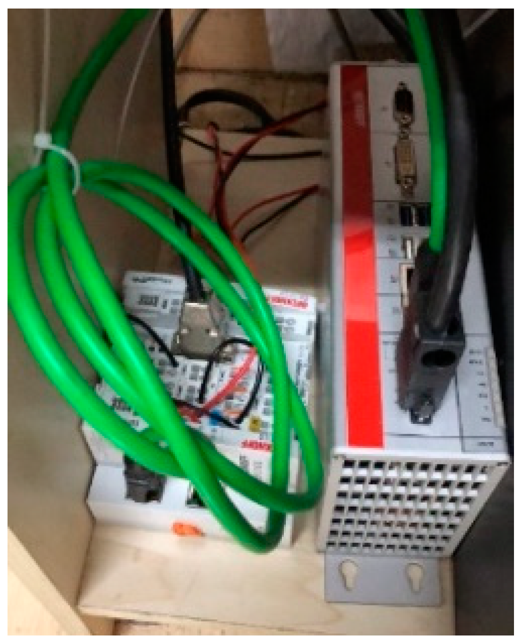
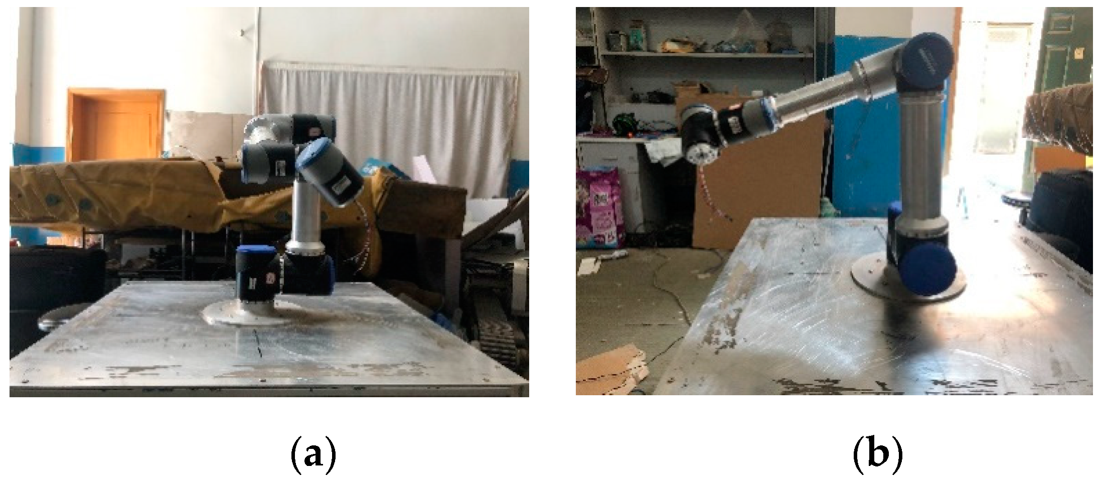
The six-DOF KingKong robot built with a Beckhoff-C6920 controller and a Kollmorgen RGM motor was used in the experiment testing the correctness and real-time performance of the algorithm. The DH parameters of the robot are listed in Table 3. The C6920 controller in Figure 5. The C6920 controller used a 32-bit Windows 7 operating system and was equipped with an Intel Core i5 processor.

Figure 6 displays the control framework for the entire system. When the controller received the order of motion, the critical parameters of the locus equation were computed according to the order. Subsequently, the position point at the next time point was planned in the Cartesian spatial planner. Based on the position points in Cartesian space, the inverse kinematics solving method proposed here was employed to obtain the position to be reached by each motor at the next time point. The closed-loop circle of the motor controller was 2 ms. The controller sent the motion order to the RGM motor via CanOpen. CanOpen is a high-level communication protocol based on the Controller Area Network. It is often used in embedded systems and is a type of field bus commonly used in industrial control.

The number of vertical joints was judged according to the KingKong DH model. Then, the algorithm assessed the first type of sub-problem. After joint decoupling was performed for $J_6$, $J_1\perp J_2\parallel J_3\parallel J_4\perp J_{5,a}$ was able to solve for ${\theta }_1$ using basic problem 3.2.1. After ${\theta }_1$ was obtained, ${}_6{}^{1}T$ and $J_2\parallel J_3\parallel J_4\perp J_{5,a}\perp J_6$ were obtained using the forward kinematics formula. At the time, the robot belonged to the second type of sub-problem and we could directly solve for ${\theta }_2+{\theta }_3+{\theta }_4,{\theta }_5\mathrm{and}{\theta }_6$. Subsequently, basic problem 3.4.2 was used to solve for ${\theta }_2\mathrm{and}{\theta }_2+{\theta }_3$ and to obtain ${\theta }_3$ and ${\theta }_4$.

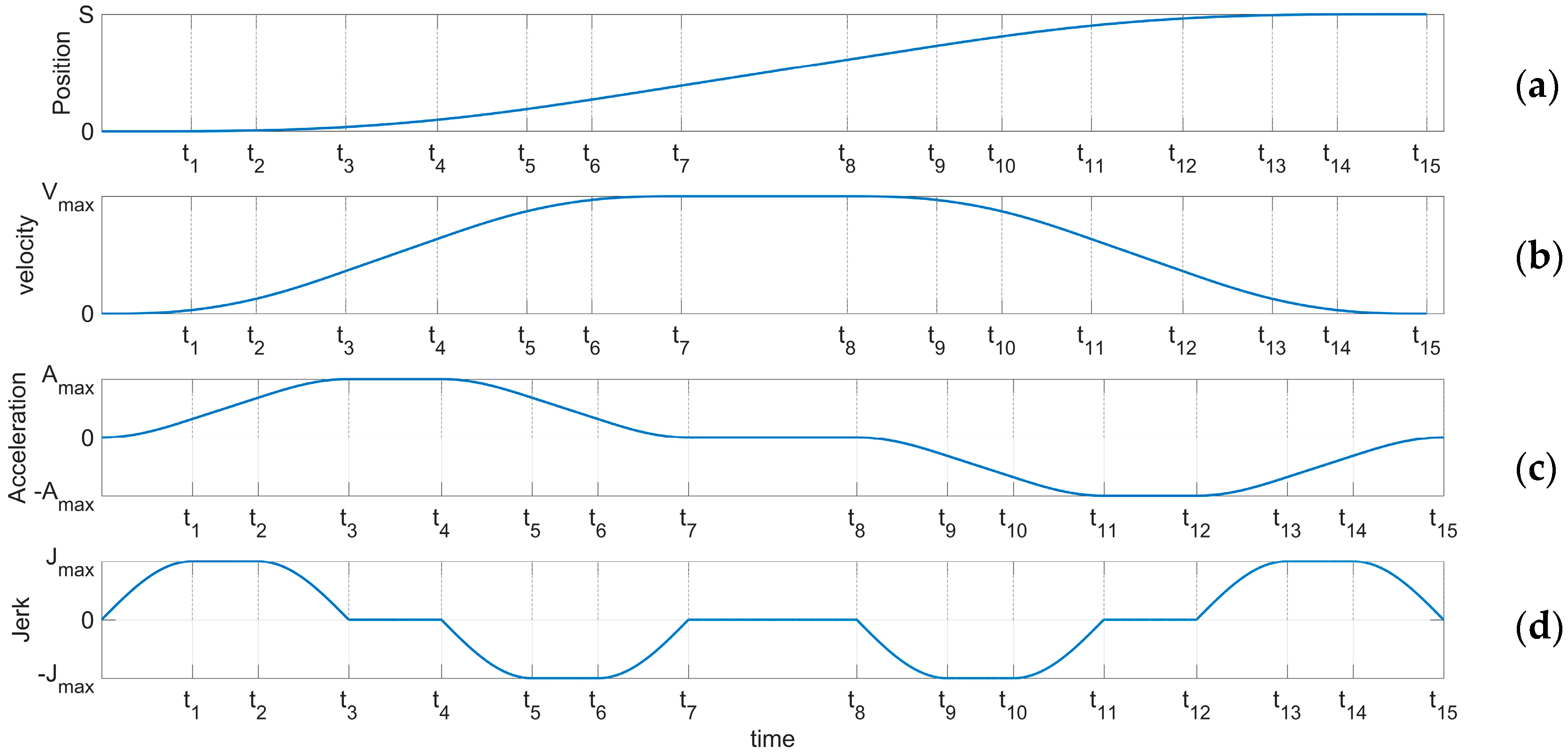
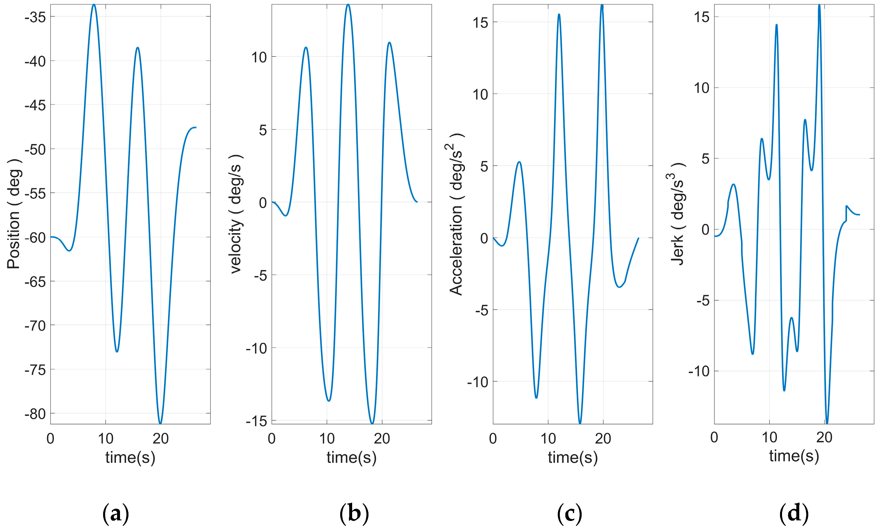
In this experiment, the robot would be commanded to move according to the specified spatial trajectory in the real environment, and the acceleration process of the motor must be considered. A common acceleration planning method is a seven-segment S curve. This method uses the square wave Jerk curve as the input of the system, and the acceleration, velocity, and position quantities obtained through the integrating of time, as is shown Figure 7.

It can be seen from the figure that the acceleration curve of the seven-segment S-curve constructed by square wave Jerk input is a linear piecewise function. Although it is continuous, but there are a finite number of non-conductible breakpoints. If the acceleration can be made to have higher order differentiable properties, the robot movement can be smoother.

In the Descartes spatial planner of the controller, the 15-segment S-curve spatial trajectory planning method was used. When the objective position, $\mathrm{S}$, and the maximum values of the curve, $\dot{S},\ddot{S},\mathrm{and}\stackrel{⃛}{S}$, are given, this method can provide a smooth curve and the speed utilization rate can approximate the optimal solution. In 15-segment S planning, the jerk input uses the sine piecewise function Equation (52) to replace the jerk square wave input in the traditional seven-segment S curve. A schematic diagram for the 15-segment S curve is shown in Figure 8.

Compared with the traditional seven-segment S curve, the 15-segment curve proposed in this paper was constructed by sinusoidal function. We know that sinusoidal functions have infinite differentiable properties. Therefore, the acceleration curve of the 15-segment S curve also has infinite differentiable properties. The curve obtained by this planning method is smoother.

$$h_n\left(t\right)=\{\begin{array}{cc}sin\frac{\pi }{2}nt& x\in \left[0,\frac{1}{n}\right]\\ 1& x\in \left[\frac{1}{n},\frac{1}{n}+m\right]\\ cos\frac{\pi }{2}n\left(t-m\right)& x\in \left[\frac{1}{n}+m,\frac{2}{n}+m\right]\end{array}.$$

(47)

In Equation (47), $n$ is an adjustable parameter to adjust the rising speed of the jerk curve and $m$ depends on the maximum values of $\ddot{S}\mathrm{and}\stackrel{⃛}{S}$.

The initial position of the KingKong robot was $\mathsf{\Theta }=\left[\begin{array}{c}0°\\ -60°\\ 120°\\ -135°\\ -45°\\ -45°\end{array}\right]$, as shown in Figure 9.

At that time, based on the forward kinematics computation, the end posture was:

$$\left[\begin{array}{cccc}-0.5536& 0.8124& 0.1830& -0.4961\\ 0.5000& 0.5000& -0.7071& -0.1330\\ -0.6660& -0.3000& -0.6830& 0.0895\\ 0& 0& 0& 1\end{array}\right].$$

(48)

The algorithm was used to obtain the inverse solution and eight sets of joint angles, as shown in

Table 19. Eight sets of reversely solved joint angles.

No.	${\mathit{\theta }}_1$/°	${\mathit{\theta }}_2$/°	${\mathit{\theta }}_3$/°	${\mathit{\theta }}_4$/°	${\mathit{\theta }}_5$/°	${\mathit{\theta }}_6$/°
1	0	38.3143	−80.0936	146.7793	45.0000	135.0000
2	0	−35.7525	80.0936	60.6588	45.0000	135.0000
3	0	47.6172	−120.0000	−2.6172	−45.0000	−45.0000
4	0	−60.0000	120.0000	−135.0000	−45.0000	−45.0000
5	−159.2347	−125.5572	−120.8932	−16.9043	136.5570	−15.1304
6	−159.2347	126.1566	120.8932	−150.4045	136.5570	−15.1304
7	−159.2347	−140.7508	−79.3110	136.7071	−136.5570	164.8696
8	−159.2347	145.8820	79.3110	51.4522	−136.5570	164.8696

. According to formula (40) the fourth set of solutions was selected and applied in the motion control logic.

The spatial planning was as follows. The experiment used a spiral line as the expected end trajectory. The parameter equation of the end trajectory spiral line is:

$$\{\begin{array}{c}x=0.15\cos \left(2\pi t\right)-0.15\\ y=0.15\sin \left(\pi t\right)\\ z=0.05t\end{array},t\in \left[0,5\right].$$

(49)

First, according to Equation (50), the arc length of the spiral line is:

$$\mathcal{l}={{\displaystyle \int }}_0^5\sqrt{{\left(\frac{dx}{dt}\right)}^2+{\left(\frac{dy}{dt}\right)}^2+{\left(\frac{dz}{dt}\right)}^2}dt=2.3694 \mathrm{m}.$$

(50)

Given ${\dot{S}}_{max}=0.125\mathrm{m}/\mathrm{s}$, ${\ddot{S}}_{max}=0.025\mathrm{m}/\mathrm{s}$, ${\stackrel{⃛}{S}}_{max}=0.01\mathrm{m}/\mathrm{s},$ and $n=1$, the 15-segment S curve was used to plan the end arc length. The total time consumed was 28.1821 s. The variation curve at each stage of the trajectory is shown in Figure 10.

The arc length obtained according to Equation (50) was used to rewrite the parametric equation:

$$\{\begin{array}{c}x=0.15\cos \left(\frac{l}{0.1581}\right)-0.15\\ y=0.15\sin \left(\frac{l}{0.1581}\right)\\ z=0.1581 l\end{array},l\in \left[0,\mathcal{l}\right].$$

(51)

In summary, the position curve in Cartesian space and its various derivatives could be obtained, together with the planned position curves of each joint and their various derivatives, as shown in Figure 11, Figure 12, Figure 13, Figure 14, Figure 15 and Figure 16.

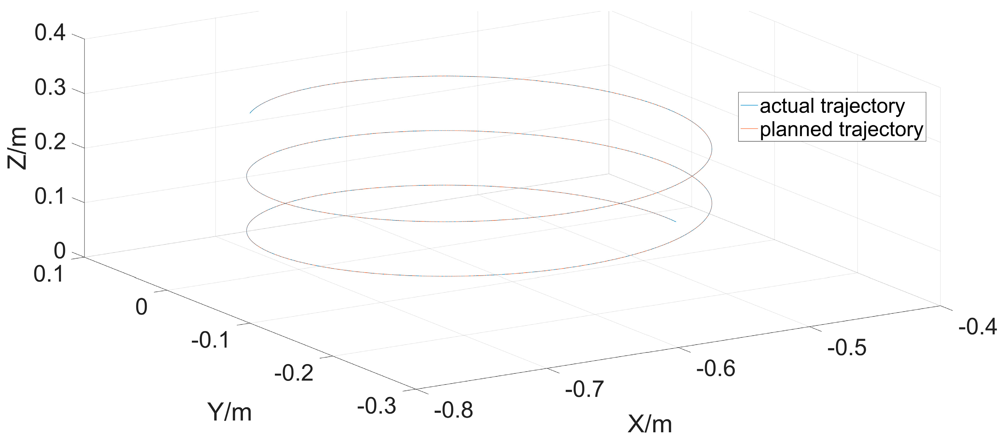
Figure 17 shows the position after the robot has finished its run. The curve of the actual motion of the robot in Cartesian space was calculated from the forward kinematics and is shown together with the planned spatial curve in Figure 18. After the run was completed, the actual motion curve of each joint was acquired from the controller, as shown in Figure 19.

In the fourth experiment, the Beckhoff controller, which is commonly used in the industry, was used and the general algorithm was implemented in the controller. The robot controller sends motion commands to the drive at a certain period. This requires the controller to complete the kinematic inverse solution within a specified amount of time to ensure the continuity. A shorter period results in a higher real-time performance. The period used in this article was 2 ms. The 2 ms cycle is sufficient to meet the general accuracy requirements. For example, in Ref. [5] the medical robot can accept a closed loop period of 20 ms. In other words, the proposed algorithm in this paper could achieve a closed-loop period higher than industrial demand in equipment commonly used in the industry. The fast closed-loop period means that the algorithm has higher computational efficiency.

Since our algorithm could decompose complex inverse motion problems into several sub-problems and solve them one by one, all joint angles could be solved accurately and quickly. The final experimental results show that the system could complete the inverse solution of the kinematics within the specified period. This allows the algorithm to run stably in situations with real-time requirements.

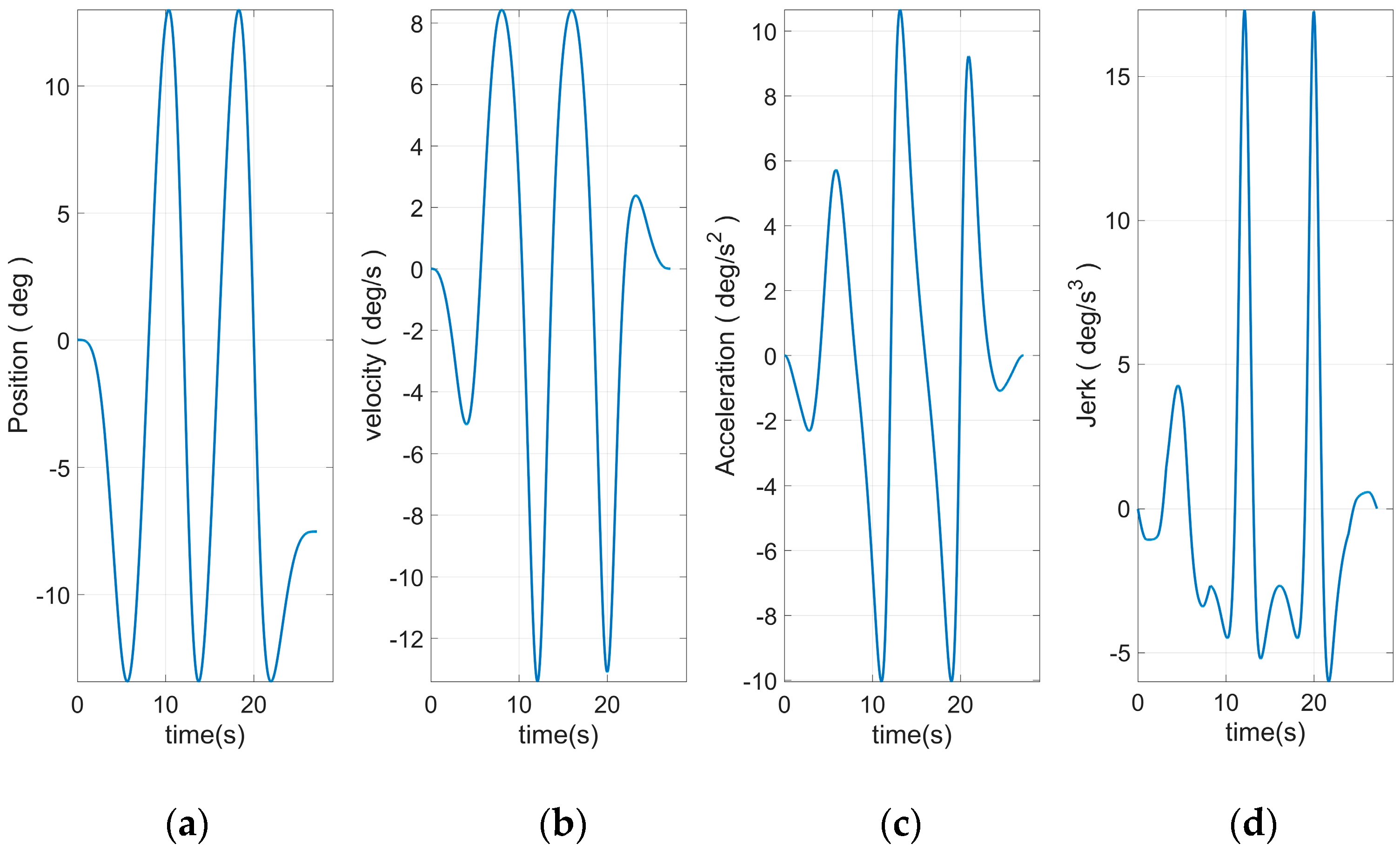
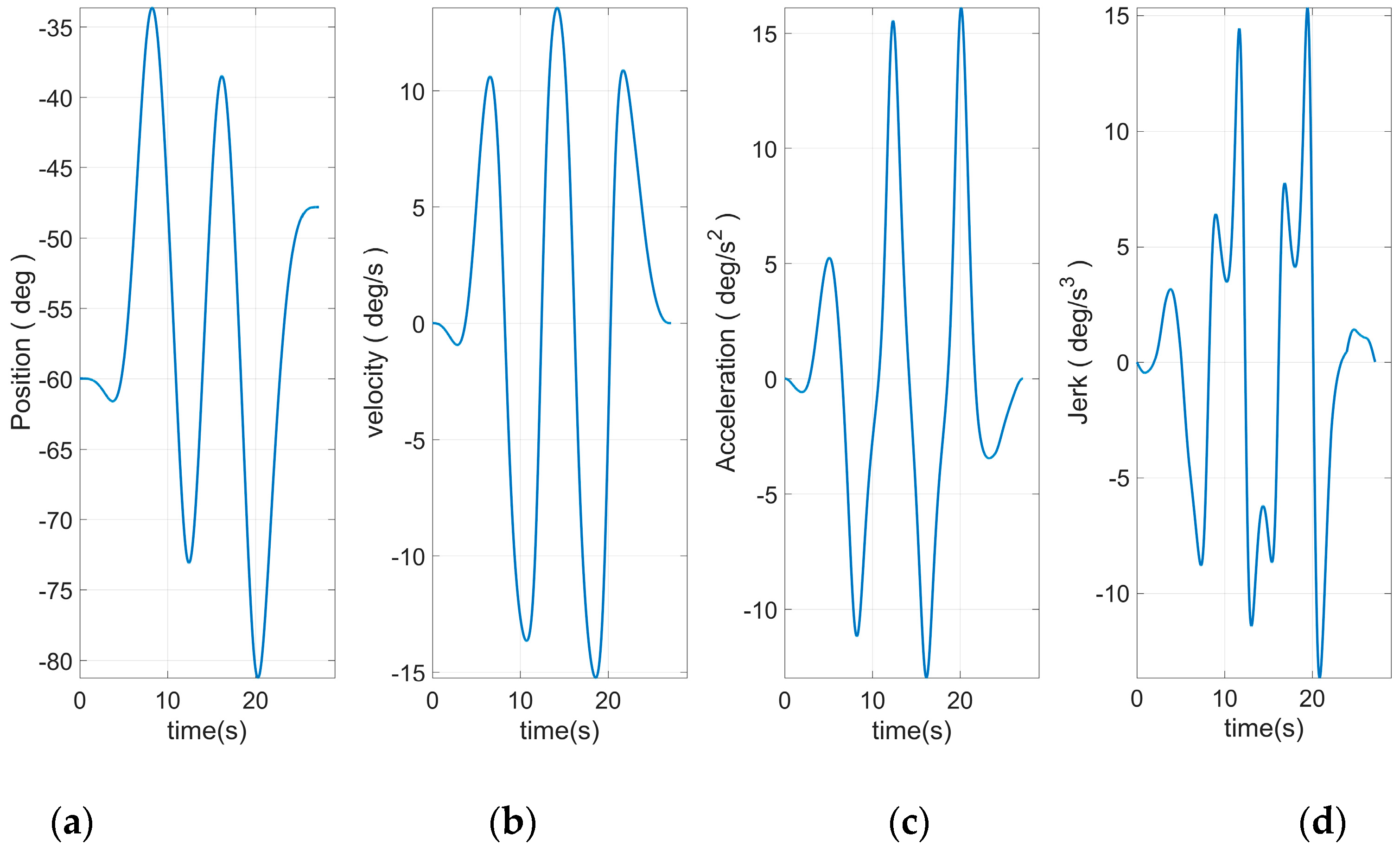
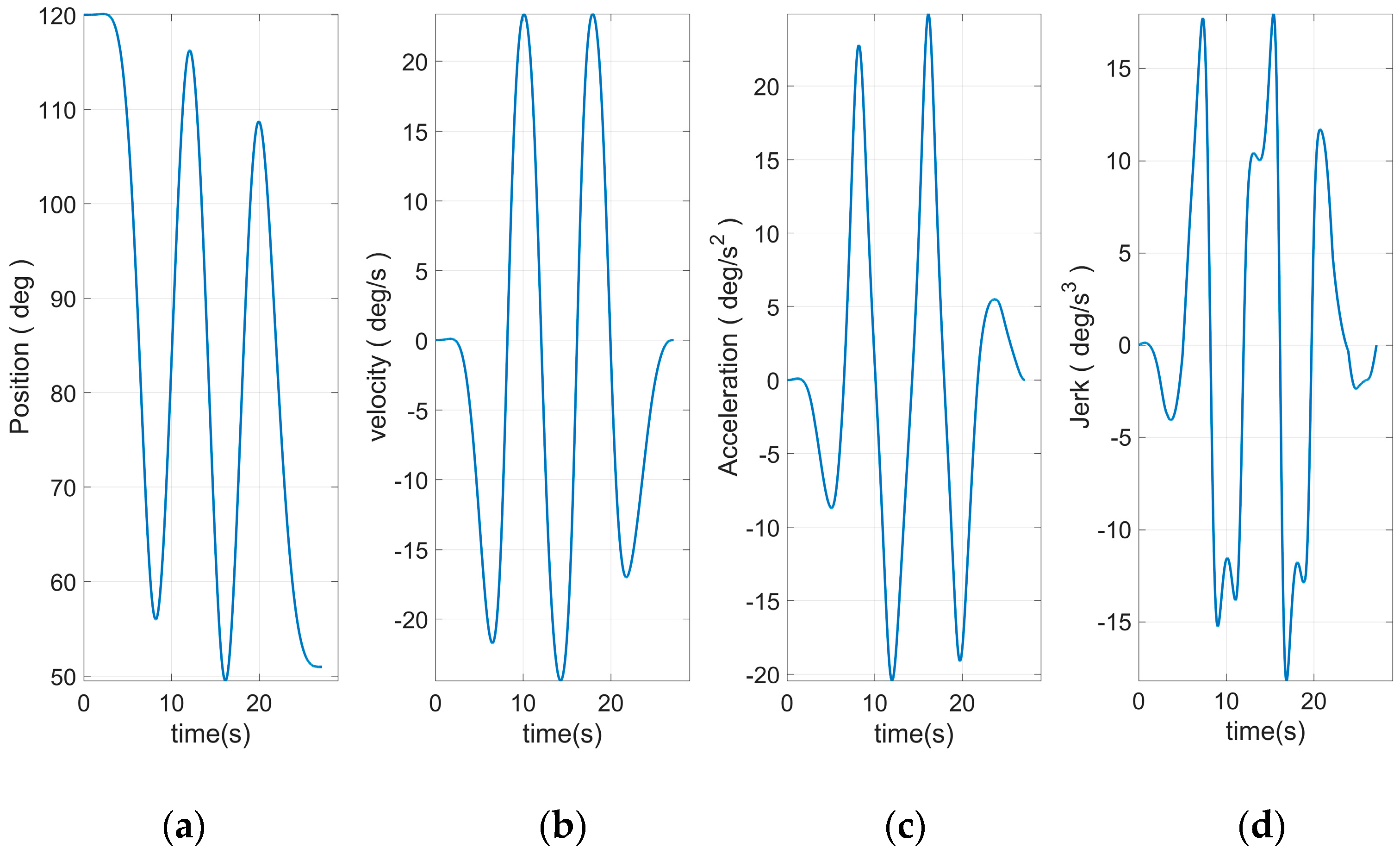
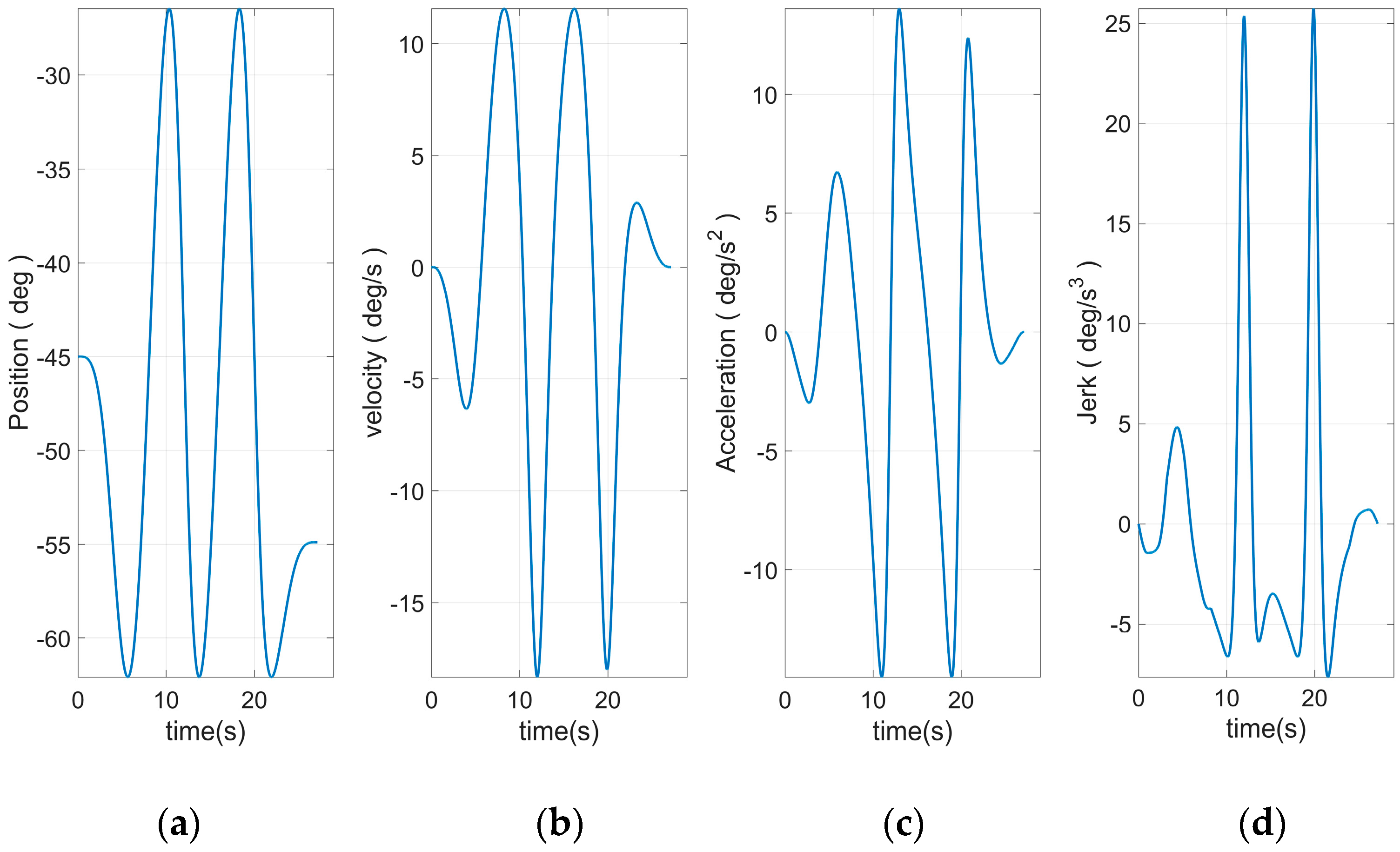
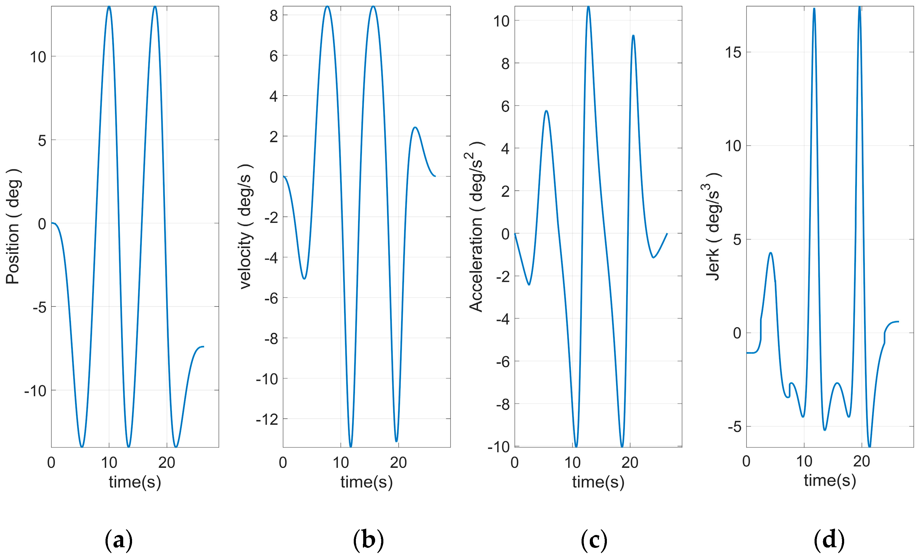
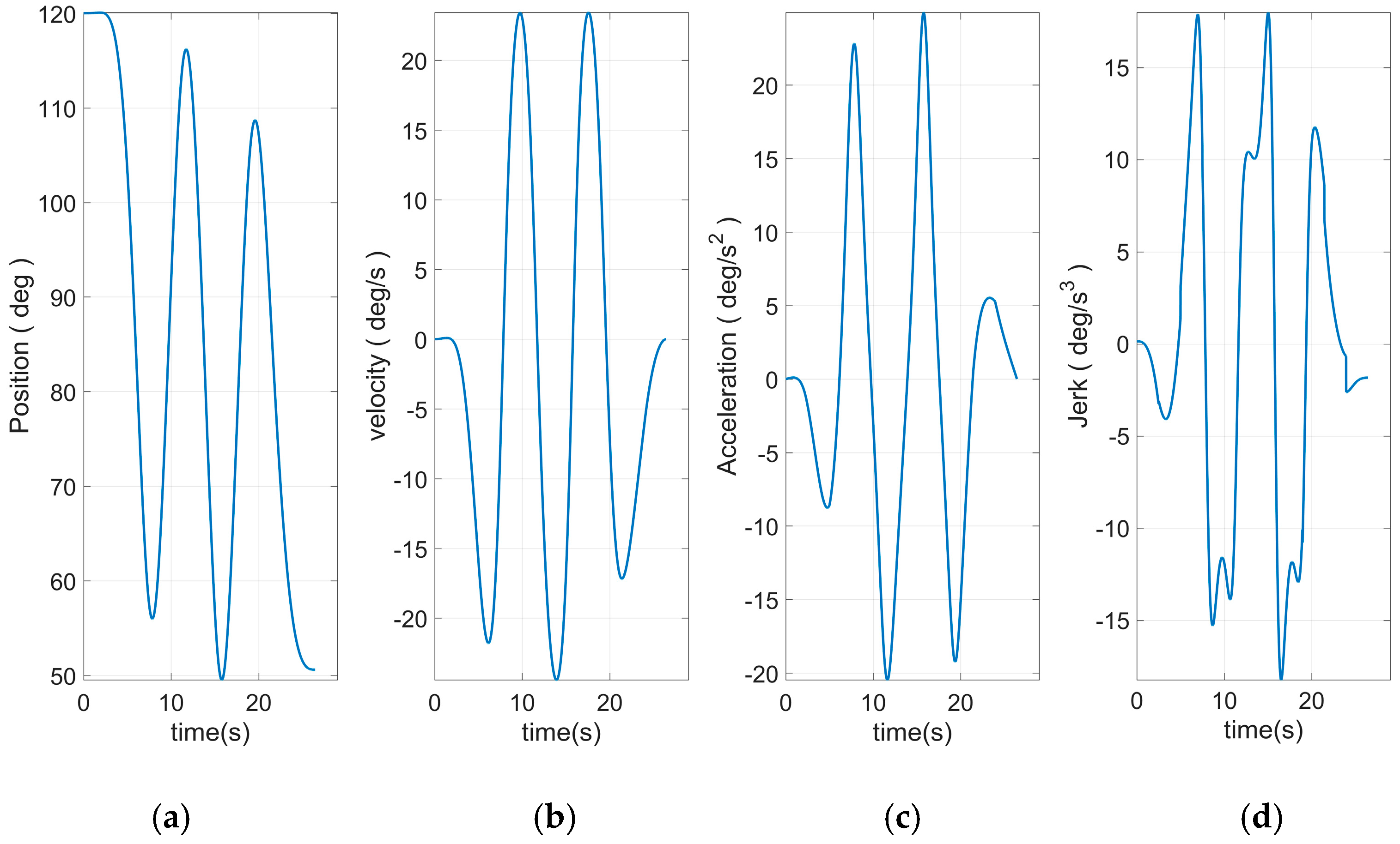
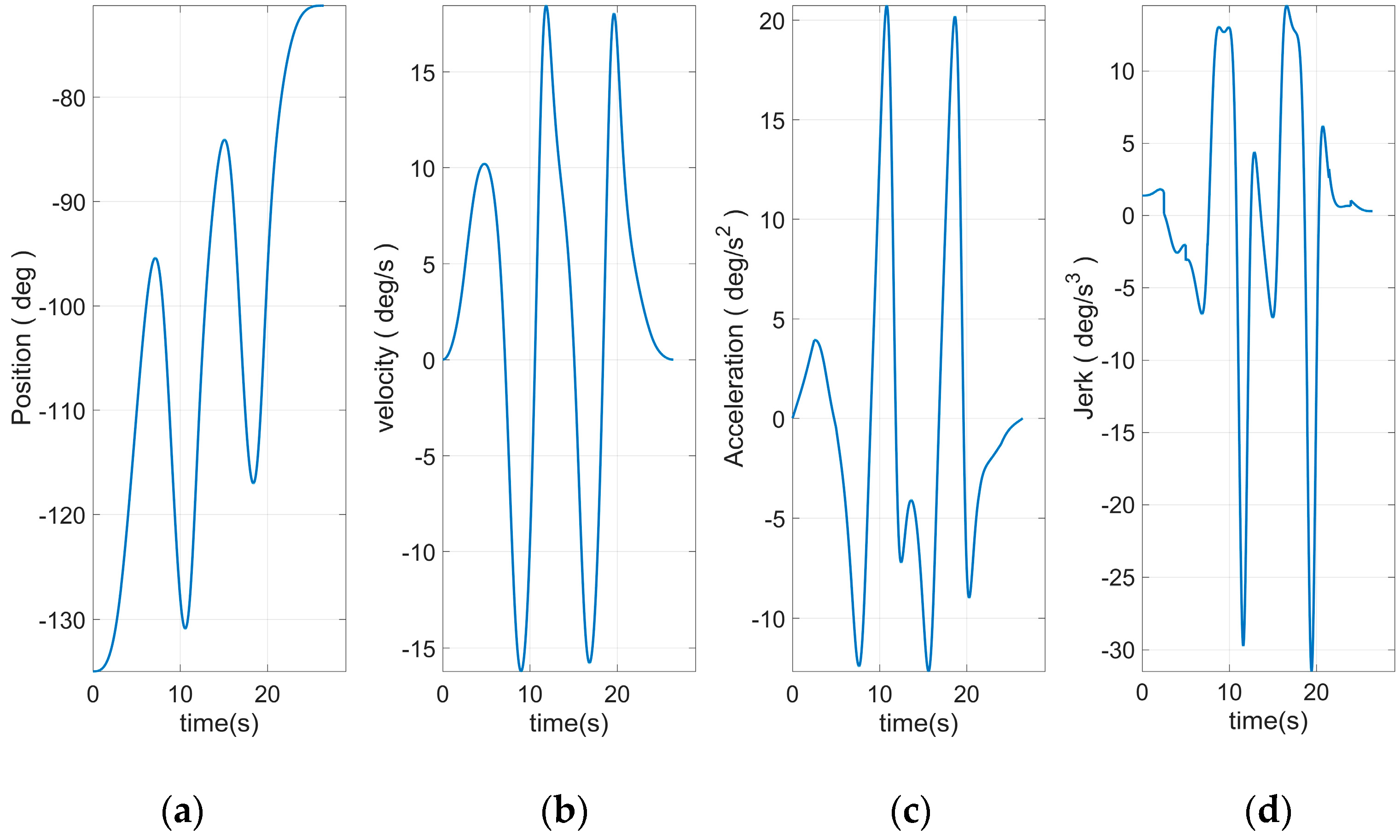
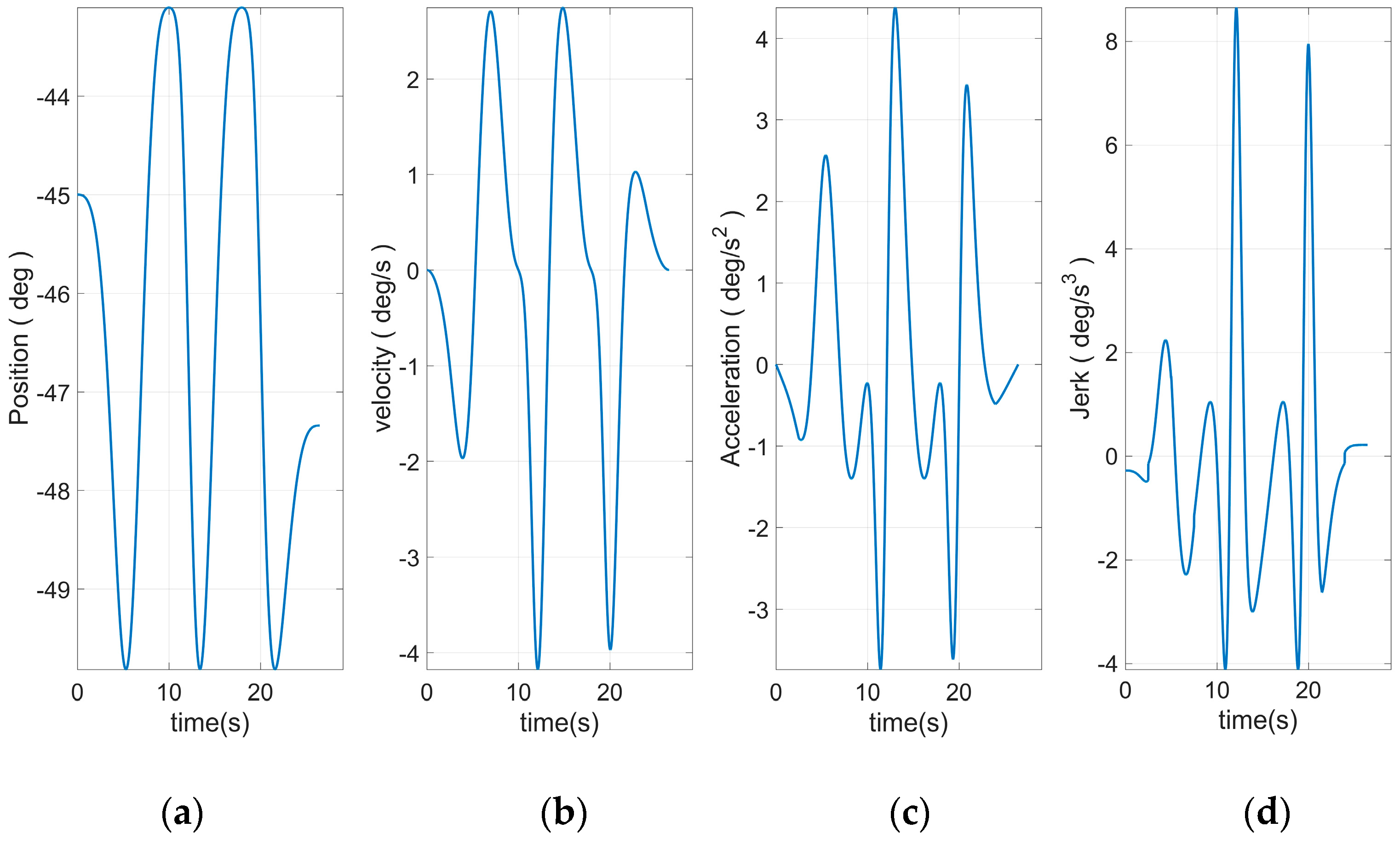
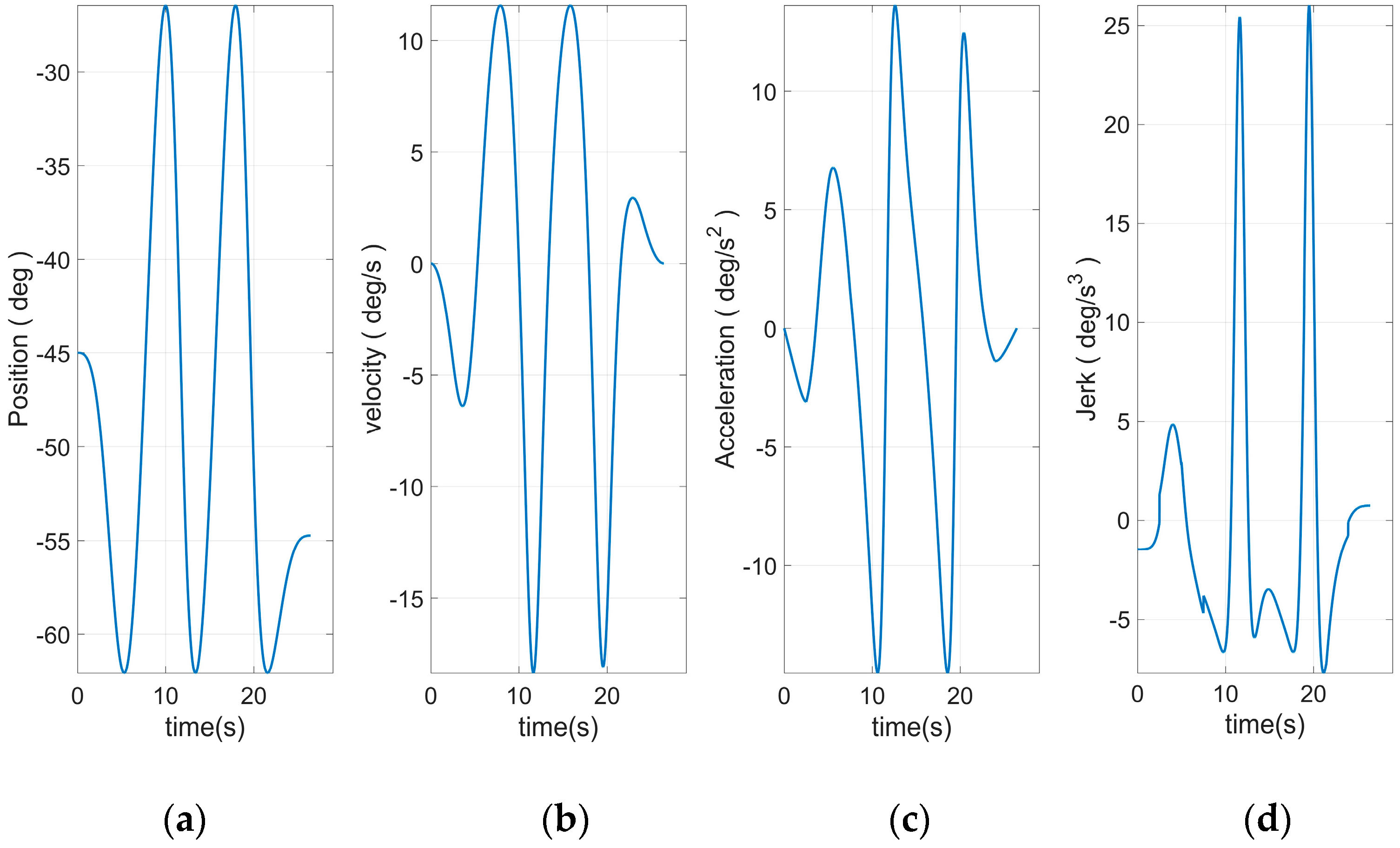
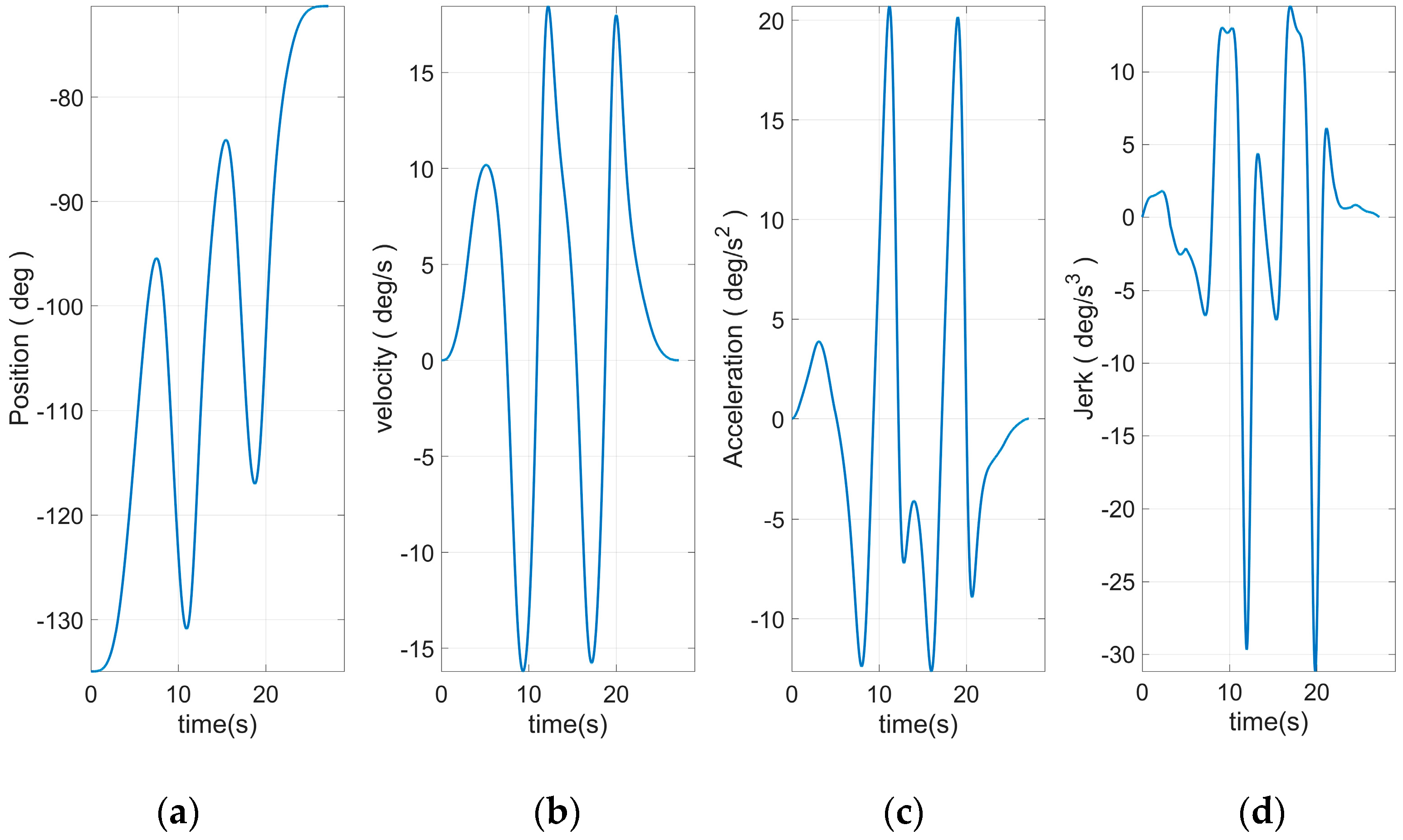
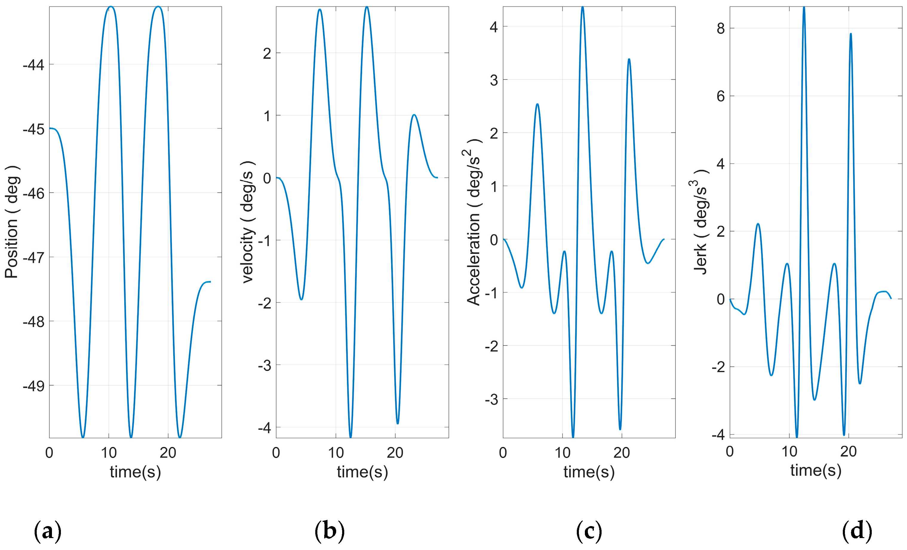
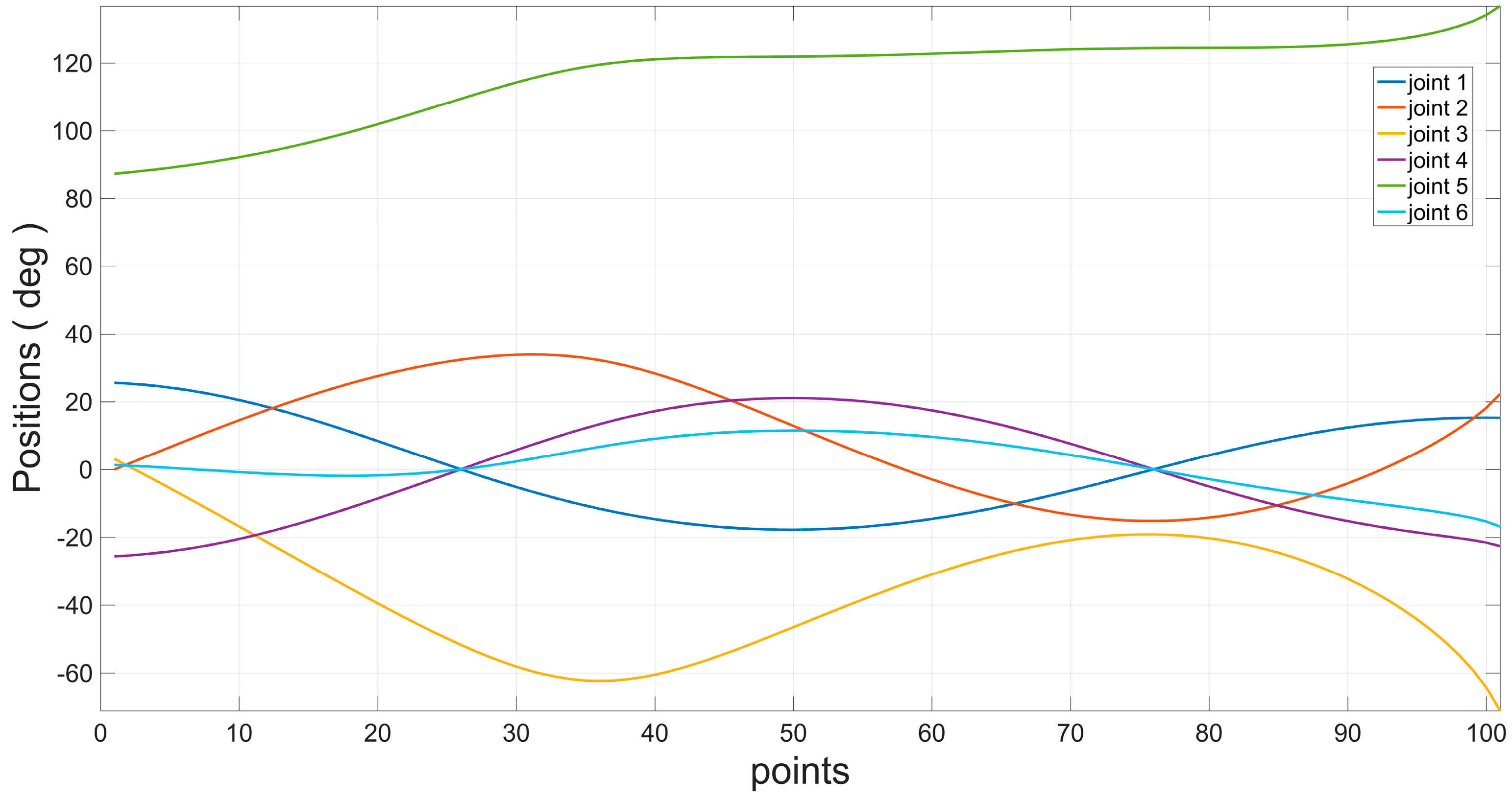
Figure 8 shows the end curve planned to use 15 S-curve segments. The apparent rise and fall process in the jerk curve could be seen. This allows the entire curve to have a smoother transition at start–stop. Based on Equation (46) and the plan in Figure 10, the angular curve of each joint could be obtained, as shown in Figure 11, Figure 12, Figure 13, Figure 14, Figure 15 and Figure 16.

It can be seen from Figure 11, Figure 12, Figure 13, Figure 14, Figure 15 and Figure 16 that all joint motion curves, as well as the various derivative curves could be ensured to start from 0 during the start-up phase smoothly. The continuous and smooth was kept in the whole moving process. Moreover, the curve was smoothly reduced to zero during the stop phase. Especially the fourth derivative had kept the continuous and smooth fluctuations, which was the effect that could not be realized through traditional planning method. This paper introduced the joint curve obtained through using the traditional seven-segment planning there to facilitate the comparison, as shown in Figure 20, Figure 21, Figure 22, Figure 23, Figure 24 and Figure 25. It can be clearly seen that the Jerk curve of each joint had an obvious jump phenomenon during the start–stop phase. Meanwhile, thumbing changes occurred in the operation process. These problems would cause the motor to operate unstably in the end.

Figure 18 shows the actual run in Cartesian space. It could be seen that the actual motion trajectory coincided with the planned motion trajectory. The mean square error of the two tracks was calculated to be 7.8265 × 10⁻¹⁰ m. This data shows that the error between the actual trajectory and the target trajectory was extremely small. This shows that the inverse solution of the robot had higher accuracy.

6. Conclusions

Based on the DH model, this study proposed a universal algorithm for finding an inverse kinematics closed-form solution. This algorithm divided the inverse kinematics problem related to robots with a closed-form solution into three sub-problems assuming that the algebraic equation had a formula solution. The solvability conditions for the three types of sub-problems were analyzed to derive a formula solution. If a serial robot can be described with these three types of sub-problems, the robot will definitely have a closed-form solution. Meanwhile, the formula solution based on such a problem could quickly solve for all the joint angles. This method was not only applicable to six-DOF robots with a closed-form solution but also to low-DOF robots with the same solution form. In addition, establishing an algorithm based on the DH model provides a concise and efficient tool for selecting sub-problems and a real-time inverse kinematics solution for the motion controller of a serial robot. To verify the correctness and real-time performance of the algorithm, we presented four experimental designs. The first three experiments were conducted on MATLAB with a series of robot to verify the completeness, universality, and continuity of this algorithm.

In the first experiment, the completeness of the algorithm was verified. The experiment used a low-degree-of-freedom robot with closed inverse solutions to prove that the algorithm could solve its closed inverse solution, and the algorithm would be terminated for the robot without closed inverse solutions to avoid infinite loop. This was used to prove the completeness of the algorithm. In the second experiment, two uncommon robots were constructed through using some basic problems, but the closed inverse solution could still be solved. Therefore, it could be known that the closed inverse solution of the series robots constructed by basic problems could be solved. Meanwhile, for these robots whose structure was not changed but the link parameter was changed, the closed inverse solution of them could also be solved correctly, which indicates that the algorithm had certain versatility in solving the closed inverse solution problem. In the third experiment, the common Puma560 robot was used as the experimental object. In the experiment, a spatial curve was planned. The correct joint angle sequence was obtained and the changes of the joint angle curve were continuously without jumping after been inversely solved by the algorithm. Which indicates that the algorithm could guarantee the continuity of its mapping on the inverse solution problem.

The fourth experiment was conducted on a six-DOF robotic platform built using a Beckhoff-C6920 controller and an RGM motor to verify the real-time performance of the algorithm using the above hardware platform. The spatial and joint positions were computed with a close-loop cycle of 2 ms and were transmitted to the motor via CanOpen. The results demonstrated the ability of the algorithm to solve the three sub-problems within a specified cycle and to compute the appropriate joint angles. Moreover, the curve was continuous. This paper used a completely new approach to study the inverse kinematics of serial robots. In this study, the conditions for the existence of the closed-form inverse kinematic solution of a serial robot were completed and the basic theory of robotics was perfected. Based on this method, a general closed-form inverse kinematics algorithm based on the DH model was implemented, which had not been done in previous studies. Importantly, this method is a general-purpose algorithm that can be used in industrial fields in real time. This increases the versatility of the universal serial robot motion controller.

However, the algorithm still has shortcomings. First, the algorithm only targets serial robots and the moving joints are not included in the solution model. This limits the scope of application of the algorithm, due to its inability to solve the cases of SCARA robots or other parallel robots. In addition, the algorithm cannot solve the problem when the robot passes through a singular point; singular points are avoided via restrictions implemented in the software. Moreover, because the algorithm is a purely analytical method, it is difficult to combine with other numerical methods to solve the problem of singular points.