Estimation Modal Parameter Variation with Respect to Internal Energy Variation Based on the Iwan Model

Abstract

Typical factors that cause nonlinear behavior in structures are geometric nonlinearity, force and displacement boundary condition nonlinearities, and material nonlinearity. The nonlinearity caused by an increase of the internal energy in built-up structures is mostly due to the displacement boundary condition induced by the contact interface region. This study proposes an experimental mode analysis technique that predicts changes in natural frequencies and damping ratios when the external excitation force increases in a structure’s contact surfaces. Specifically, the nonlinearity of the dynamic characteristics induced by the contact region is described by the constitutive Iwan model. Next, an estimation method was developed for two parameters among the four of the Iwan model. This study used a modal analysis method. As an extension of a previous study, the approximate form of the harmonic excitation-induced force was determined in closed form. The configuration of the numerical model for the full structure was introduced from this resultant form. By using these numerical results, responses in the full structure, according to the harmonic excitation, have been represented in mode summation form. This research proposes an estimation method for two parameters among the four of the constitutive model. The proposed method was verified by simulations conducted with the lumped model and by experiments conducted on a partially connected double beam.

1. Introduction

Generally, experimental modal analysis was performed to ensure structural stability under operating conditions. The structure’s stability under dynamic conditions was evaluated based upon the identified modal parameters, such as the natural frequency, mode shape, and damping ratio. However, most mechanical structures do not operate under steady-state conditions; moreover, the operating frequency varies with the magnitude of the excitation force [1,2]. In vibration analysis, an increase in the external force is interpreted as an increase in the internal energy, which changes the dynamic characteristics [3]. Finally, a nonlinear analysis of the structure is required. Nonlinearities are typically divided into geometric nonlinearities [4], force and displacement boundary conditions [5], and material nonlinearities [6]. The nonlinearity due to an increase in the internal energy of the general built-up structure is mostly due to a displacement boundary condition induced by the contact region inside the structure [7,8]. The study proposes a methodology for predicting changes in the natural frequency and damping ratio when the external force increases in a built-up structure with contact surfaces. Specifically, the frequency response function (FRF) in the modal domain is derived based on the Iwan model, which is a representative constitutive model describing the nonlinearity of the dynamic characteristics due to the contact surfaces. Based on the derived FRF, the natural frequencies and damping ratios at a certain magnitude of excitation force or internal energy are predicted.

The Iwan model, which was introduced by Iwan [9,10], is composed of Jenkins elements of a spring-slider unit in a parallel series, where the slider represents Coulomb friction. In this model, the hysteretic behavioral effect within the structural force-displacement curve is an approximate bilinear model. Segalman et al. [11] extensively reviewed this model and applied it to a finite element (FE) model, which was the initial striving for Iwan model application to describe the dynamic tangential responses of lap joints. Segalman et al. expressed the Iwan model with four parameters in [12] and attempted to account for the dynamic behavior at the interface between the micro-slip and macro-slip regimes using the Dirac delta function. This four-parameter Iwan model is commonly used for the non-linear behavioral model of bolted joints in the micro-slip regime. In addition, a follow-up study analyzed this model in the modal domain [13], where the interface’s influence on each model was considered, leading to a decoupled set of modal equations. These modal equations were a collection of parallel-series Iwan models that were used to determine the contribution of the joints to each mode. Recently, the Iwan model was used to represent built-up structures [14,15,16]. These studies confirmed that each mode had a different effect on the Iwan model and introduced an order reduction possibility for the full FE model of the structure.

In this study, as an extension of [13], two parameters (R, χ), out of the four introduced in [12], were estimated by modal analysis. Further, the steady state response of the Iwan model was investigated in the modal domain and the conventional modal parameter estimation method was applied to the results. The other two parameters were related to the reference position, which distinguished the micro-slip and macro-slip in the Iwan model and the backbone’s curvature at the reference position. When only in the dynamic state in the micro-slip region, the structure of interest is not considered for the study as the parameters will have no effect. To estimate the change in the resonance frequency and damping ratio with respect to an increase in the external force or internal energy, the equation of motion for the built-up structure was derived by assuming that the contact surface was connected to the Iwan model. An experimental modal analysis was proposed to predict the two parameters using the derived equation of motion in the modal domain.

Section 2 describes the Iwan model. In Section 2.1, the mathematical model of the generated force in the Iwan model is described. In Section 2.2, the equation of motion in the modal domain is derived for the general built-up structure in which contact surfaces are represented by the Iwan model. Further, an experimental modal analysis is introduced for estimating the two proposed parameters. In Section 3, the effectiveness of the proposed method is demonstrated using the lumped mass model. In Section 4, the proposed method is experimentally verified. This study proposes a method to identify two parameters, out of the four parameters of the Iwan model, which are used to describe the change of dynamic characteristics according to changes in the internal energy of the built-up structures. The other two parameters are not required when the structure is in the micro-slip regime. In general, quasi-static experiments are performed to identify these two parameters. For parameter identification, the Iwan model is transformed into modal domain as modal equations. By using the derived modal equations, an attempt is made to estimate the two parameters by applying experimental modal analysis, which is generally performed to identify the dynamic characteristics of the structures.

To verify the proposed method, the FRFs for a partially connected double beam structure with ends attached using glue were measured while the structure was excited by ten consecutively increasing forces. The resonance frequencies and damping ratios were confirmed by applying the commercial modal parameter estimation method to the measured FRFs. Two parameters of the Iwan model were estimated by applying the proposed method to the measurements from the first seven experiments. The resonance frequencies and damping ratios were estimated for the remaining three forces based on the two estimated parameters. The results were compared with the estimated modal parameters from experimental measurements.

2. Theory

2.1. Modeling of Joint Force

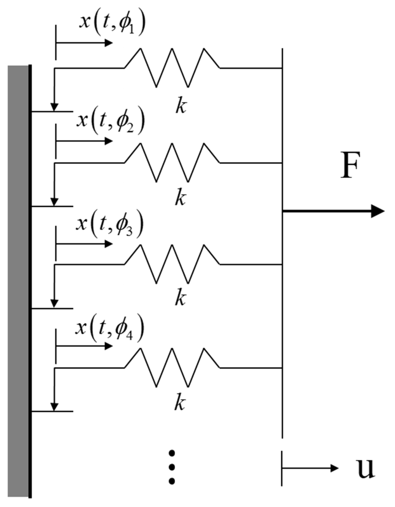
Figure 1 shows the parallel-series Iwan model that has an equivalent stiffness k. The mathematical description of this model is as follows:

$$F\left(t\right)={{\displaystyle \int }}_0^{\infty }\rho \left(\varphi \right)\left[u\left(t\right)-x\left(t,\varphi \right)\right]d\varphi$$

(1)

In Equation (1), F denotes the applied force. $\varphi$ denotes the sliding distance of each element and $\rho \left(\varphi \right)$ denotes the population density of Jenkins element of strength $\varphi$. u denotes the imposed distance and x denotes the slider displacement. Each quantity has the following dimensions. F has the dimension of force (N). $\varphi$, u and x have the dimension of length (m). The slider displacement x(t,$\varphi$) evolves from the imposed displacement u(t).

$$\dot{x}\left(t,\varphi \right)=\{\begin{array}{c}\dot{u}\\ 0\end{array}\begin{array}{c}if\Vert u-x\left(t,\varphi \right)\Vert =\varphi \mathrm{and}\dot{u}\left[u-x\left(t,\varphi \right)\right]>0\\ \mathrm{otherwise}\end{array}$$

(2)

In Equation (2), $\dot{x}$ and $\dot{u}$ represent the slider velocity and the imposed velocity, respectively. If u is subject to frequency ω and amplitude A, it means

$$u\left(t\right)=Asin\omega t$$

(3)

Then, Equation (1) can be represented as follows:

$$F\left(t\right)={{\displaystyle \int }}_0^A\rho \left(\varphi \right)\left[u\left(t\right)-x\left(t,\varphi \right)\right]d\varphi +{{\displaystyle \int }}_A^{\infty }\rho \left(\varphi \right)u\left(t\right)d\varphi$$

(4)

The second term on the right-hand side of Equation (4) can be obtained because $x\left(t,\varphi \right)=0$ for all $\varphi$ > A. If one re-arranges Equation (4),

$$F\left(t\right)=u\left(t\right)K_T-\Delta F_S\left(t\right)$$

(5)

$\mathrm{where}{K}_T={{\displaystyle \int }}_0^{\infty }\rho \left(\varphi \right)d\varphi ,\mathsf{\Delta }{F}_S\left(t\right)={{\displaystyle \int }}_0^A\rho \left(\varphi \right)x\left(t,\varphi \right)d\varphi \mathrm{and} u\left(t\right)=Asin\left(\omega t-\theta \right)$.

In Equation (5), K_T represents the added stiffness by joints in built-up structures. △F_S represents the variation force for the occurring slip. We adopt the representation of the density function $\rho$ in Reference [12] to investigate in more detail the result in this equation; this representation is composed of the 4 parameters and is shown below:

$$\rho \left(\varphi \right)=R{\varphi }^{\chi }[H\left(\varphi \right)-H(\varphi -\varphi ma{x}_{max})]$$

(6)

In Equation (6), R, χ, ${\varphi }_{max}$ and S are four parameters that describe the density function. Here, R is the parameter related to the magnitude of the density function. χ is a constant, which has a value between −1 and 0. ${\varphi }_{max}$ is a constant representing the border line that determines the micro-slip and macro-slip in the contact surfaces of two objects. S is a constant to describe the dynamic characteristics when macro-slip occurs. In addition, H and δ in this equation represent the Heaviside function and the Dirac delta function, respectively. These four parameters {R, χ, ${\varphi }_{max}$ and S} can be transformed into the following four parameters {χ, K_T, F_S and β}. In these newly introduced parameters, χ is the existing parameter in the original set and K_T represents the introduced added stiffness by joint in Equation (4). The other remaining parameters have the following relations [12]:

$$F_s\left(t\right)=u\left(t\right){{\displaystyle \int }}_0^{\infty }\rho \left(\varphi \right)d\varphi \mathrm{and}\beta =\frac{S}{\left(\frac{R{\varphi }_{max}^{\chi }}{\chi +1}\right)}$$

(7)

In the results of Equation. (7), F_S represents the critical force to generate macro-slip. β is the constant related to the curvature in the backbone curve. If one assumes that the constitutive model in Equation. (3) behaves in the micro-slip region, then the variation force in Equation. (5) can be represented as the following:

$$\Delta F_S\left(t\right)={{\displaystyle \int }}_0^A\rho \left(\varphi \right)x\left(t,\varphi \right)d\varphi ={{\displaystyle \int }}_0^{A}x\left(t,\varphi \right)R{\varphi }^{\chi }d\varphi$$

(8)

In Equation (8), the slider displacement x is related to the imposed velocity $\dot{u}$ as follows [9,13]:

$$\begin{array}{l}\mathrm{for}\dot{u}>0\\ x=\{\begin{array}{c}u-\varphi \\ -A+\varphi \end{array}\begin{array}{c}for0<\varphi <\left(u+A\right)/2\\ for\left(u+A\right)/2<\varphi <A\end{array}\end{array}$$

(9a)

$$\begin{array}{l}\mathrm{for}\dot{u}<0\\ x=\{\begin{array}{c}u+\varphi \\ A-\varphi \end{array}\begin{array}{c}for0<\varphi <\left(A-u\right)/2\\ for\left(A-u\right)/2<\varphi <A\end{array}\end{array}$$

(9b)

Substituting Equation (9) in Equation (8), then,

$$\Delta F_s^{+}\left(t\right)=R\frac{{(u+A)}^{\chi +2}\cdot 2^{-\left(\chi +1\right)}-A^{\chi +2}}{\left(\chi +1\right)\left(\chi +2\right)}$$

(10a)

$$\Delta F_s^{-}\left(t\right)=-R\frac{{(A-u)}^{\chi +2}\cdot 2^{-\left(\chi +1\right)}-A^{\chi +2}}{\left(\chi +1\right)\left(\chi +2\right)}$$

(10b)

In Equation (10), the superscripts + and – refer to the moment when $\dot{u}$ has positive and negative values, respectively. If one substitutes Equation (3) into the results of Equation (10), then,

$$\Delta F_s\left(t\right)=\{\begin{array}{c}\Delta F_s^{+}\left(t\right)={\gamma }_1{(1+sin\omega t)}^{\chi +2}-{\gamma }_2\mathrm{when}-\frac{T}{4}<t<\frac{T}{4}\\ \Delta F_s^{-}\left(t\right)=-{\gamma }_1{(1-sin\omega t)}^{\chi +2}+{\gamma }_2\mathrm{when}-\frac{T}{2}<t<-\frac{T}{4}\mathrm{and}\frac{T}{4}<t<\frac{T}{2}\end{array}$$

(11)

$\mathrm{where}{\gamma }_1=D\cdot A^{\chi +2}\cdot 2^{-\left(\chi +1\right)},{\gamma }_2=D\cdot A^{\chi +2}\mathrm{and}D=\frac{R}{\left(\chi +1\right)\left(\chi +2\right)}$.

If one attempts to represent the variation force for one period, as shown in Equation (11), which is divided into two regions in the time domain by a Fourier series, the following is obtained:

$$\Delta F_s\left(t\right)=\frac{1}{2}{a}_0+{\displaystyle \sum }_{n=1}^{\infty }{a}_{n}cosn\omega t+{\displaystyle \sum }_{n=1}^{\infty }{b}_{n}sinn\omega t$$

(12)

where

$$\begin{array}{l}{a}_0=\frac{2}{T}{{\displaystyle \int }}_{-T/2}^{T/2}\Delta F_s\left(t\right)dt\\ a_n=\frac{2}{T}{{\displaystyle \int }}_{-T/2}^{T/2}\Delta F_s\left(t\right)\cdot cosn\omega tdt\\ b_n=\frac{2}{T}{{\displaystyle \int }}_{-T/2}^{T/2}\Delta F_s\left(t\right)\cdot sinn\omega tdt\end{array}$$

(13)

Equation (12) shows the variation force, which is represented in the Fourier series. Equation (13) shows the forms of every coefficient of this equation. In Equation (13), T denotes one period of time (i.e., T = 2π/ω). If one applies Equation (11) to Equation (12) and represents the variation force using only the fundamental frequency component (i.e., the first harmonic component), then the following result can be obtained (a detailed description on how to obtain this result is in Appendix A):

$$\Delta F_s\left(t\right)\cong a_{1}cos\omega t+b_{1}sin\omega t=A^{\chi +2}\left\{{\kappa }_1\left(\chi \right)cos\omega t+{\kappa }_2\left(\chi \right)sin\omega t\right\}$$

(14)

Configurations of ${\kappa }_1$ and ${\kappa }_2$ in Equation (14) refer to Equation (A15). If one considers the more practical case of the imposed displacement compared to the case in Equation (3),

$$u\left(t\right)=Asin\left(\omega t-\theta \right)$$

(15)

The variation force with respect to the case in Equation (15) can be obtained as follows if one follows a similar procedure to obtain the result in Equation (14).

$$\Delta F_s\left(t\right)=A^{\chi +1}\left\{{\kappa }_2\left(\chi \right)Asin\left(\omega t-\theta \right)+{\kappa }_1\left(\chi \right)Acos\left(\omega t-\theta \right)\right\}$$

(16)

Re-representing Equation (16) after substituting Equation (15) into this equation, produces the following:

$$\Delta F_s\left(t\right)=A^{\chi +1}\left\{{\kappa }_2\left(\chi \right)u\left(t\right)+{\kappa }_1\left(\chi \right)\frac{\dot{u}\left(t\right)}{\omega }\right\}$$

(17)

It can be confirmed from Equation (A15) that ${\kappa }_1$ and ${\kappa }_2$ will have negative and positive values, respectively. Therefore, one can re-represent Equation (17) as follows:

$$\Delta F_s\left(t\right)=A^{\chi +1}\left\{{\kappa }_2\left(\chi \right)u-\left|{\kappa }_1\left(\chi \right)\right|\frac{\dot{u}}{\omega }\right\}$$

(18)

The above equation approximately represents the induced force when harmonic dynamic behavior occurs in the constitutive model.

2.2. Modal Formulation of the Full Structure

In this section, the configuration of the variation force, which is generated in the constitutive model during dynamic behavior, is examined through a 2 degrees-of-freedom (DOF) system. In addition, this result is extended to a multi-degree-of-freedom system, which involves the constitutive model. The configuration of the FRF for this system with respect to the harmonic excitation is obtained. The methodology, which is intended in this study to estimate certain parameters out of the parameters of the constitutive model, is introduced through these results.

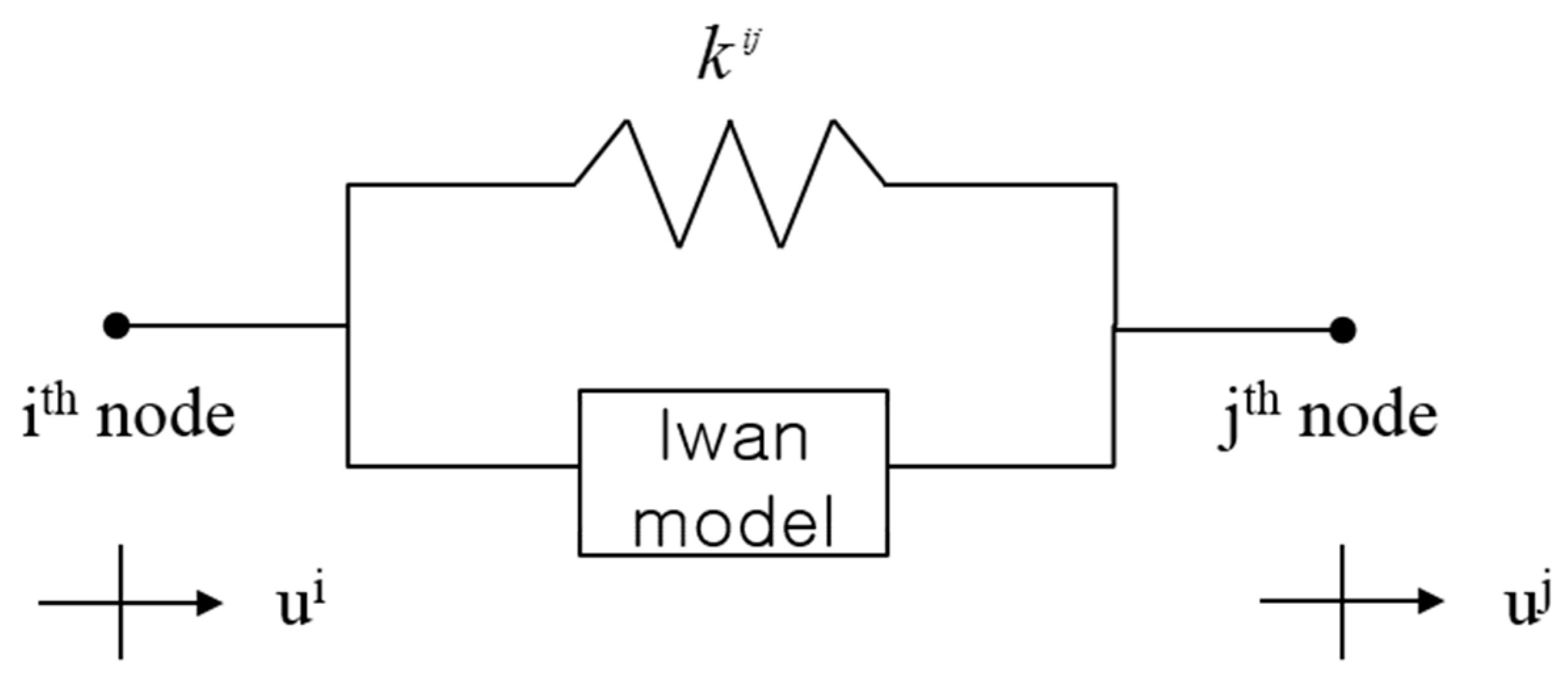
Figure 2 represents a 2 DOF system, which is connected by the stiffness k^ij and the Iwan model. Here, uⁱ and u^j represent the displacement at each node. The relative displacement between these two nodes when an external force is applied can be represented as follows:

$$u=u^j-u^i=A_{ij}sin\left(\omega t-\theta \right)$$

(19)

In Equation (19), $A_{ij}$ denotes the amplitude of the relative displacement between the i^th and j^th nodes. By using this equation, the restoring force in the stiffness and the generating force in the Iwan model can be represented in vector-matrix form using Equations (5) and (18):

$${\mathit{f}}_r^{ij}=-{\mathit{K}}^{ij}{\mathit{u}}^{ij},\left\{\begin{array}{c}{f}_r^i\\ f_r^j\end{array}\right\}=-\left[\begin{array}{cc}{k}^{ij}& -k^{ij}\\ -k^{ij}& k^{ij}\end{array}\right]\left\{\begin{array}{c}{u}^i\\ u^j\end{array}\right\}$$

(20)

$${\mathit{f}}_J^{ij}=-{\mathit{K}}_T^{ij}{\mathit{u}}^{ij}+\Delta {\mathit{f}}_s^{ij}$$

(21)

where

$$\begin{gathered} {\mathit{K}}_T^{ij}=\left[\begin{array}{cc}{K}_T^{ij}& -K_T^{ij}\\ -K_T^{ij}& K_T^{ij}\end{array}\right],{\mathit{u}}^{ij}=\left\{\begin{array}{c}{u}^i\\ u^j\end{array}\right\} \\ and \\ \Delta {\mathit{f}}_s^{ij}=-\frac{\left|{\kappa }_1\right|}{\omega }{\mathit{A}}_{ij}{\dot{\mathit{u}}}^{ij}+{\kappa }_2{\mathit{A}}_{ij}{\mathit{u}}^{ij}\mathrm{or}\left\{\begin{array}{c}\Delta f_s^i\\ \Delta f_s^j\end{array}\right\}=-\frac{\left|{\kappa }_1\right|}{\omega }\left[\begin{array}{cc}{A}_{ij}^{\chi +1}& -A_{ij}^{\chi +1}\\ -A_{ij}^{\chi +1}& A_{ij}^{\chi +1}\end{array}\right]\left\{\begin{array}{c}{\dot{u}}^i\\ {\dot{u}}^j\end{array}\right\}+{\kappa }_2\left[\begin{array}{cc}{A}_{ij}^{\chi +1}& -A_{ij}^{\chi +1}\\ -A_{ij}^{\chi +1}& A_{ij}^{\chi +1}\end{array}\right]\left\{\begin{array}{c}{u}^i\\ u^j\end{array}\right\} \end{gathered}$$

(22)

Equations (20) and (21) represent the restoring force in the stiffness and the variation force in the constitutive model when an external force is applied, respectively. Detailed configurations on each element of Equation. (21) are introduced in Equation. (22). In this equation, the matrix ${\mathit{K}}_T^{ij}$ denotes a matrix that is composed of combinations of the added stiffness (K_T) by joints, which is one of the parameters defining the Iwan model. The matrix ${\mathit{A}}_{ij}$ denotes a matrix that is composed of the combinations of relative displacement between nodes. Actually, the results in these equations can be extended without a loss of generality for general built-up structures. This means that the results of Equations (20)–(22) can be regarded as the local matrix for the interface between the jointed surfaces of general built-up structures. If one represents the equilibrium of force in general built-up structures by a vector summation form according to the Newton’s second law, then,

$${\mathit{f}}_I={\mathit{f}}_e+{\mathit{f}}_c+{\mathit{f}}_r+{\mathit{f}}_J$$

(23)

In Equation. (23), the subscripts I, e, c, r and J denote the force by inertia, the external force, the force by damping, the restoring force by stiffness and the force occurring in the joint component, respectively. If the equation of motion for the full structure is represented with this equation, then the following is obtained:

$$\mathit{M}\ddot{\mathit{u}}+\mathit{C}\dot{\mathit{u}}+\mathit{K}\mathit{u}={\mathit{f}}_e-{\mathit{K}}_T\mathit{u}-\frac{\left|{\kappa }_1\right|}{\omega }\mathit{A}\dot{\mathit{u}}+{\kappa }_2\mathit{A}\mathit{u}$$

(24)

On the left side of Equation (24), M, C and K denote the mass, damping and stiffness matrices for the full system, respectively. Note that, in general, there are multiple numbers of joint components in the built-up structures. Therefore, as mentioned in [13], “if one wants to estimate information on a certain constitutive model for a certain joint, the other joint components should be excepted from the full built-up structures apart from the joint component of interest”. Hence, the numerical model for the full structure, which includes the joint component shown in Equation (24), indicates that only the joint component of interest is connected in the full system. In this study, the full system stands for the same meaning of this statement. On the right side of Equation (24), every term apart from the external forcing vector ${\mathit{f}}_e$ represents forces generated from the joint in a global coordinate system. In particular, matrices ${\mathit{K}}_T$ and $\mathit{A}$ are all of the symmetric matrices and are composed of real values. Re-arranging Equation (24) after transferring all of the terms in the right hand side of the equation apart from the term in the external forcing vector to the left side produces the following:

$$\mathit{M}\ddot{\mathit{u}}+\left(\mathit{C}+\frac{\left|{\kappa }_1\right|}{\omega }\mathit{A}\right)\dot{\mathit{u}}+\left({\mathit{K}}_J-{\kappa }_2\mathit{A}\right)\mathit{u}={\mathit{f}}_e$$

(25)

where $K_J=K+K_T$.

${\mathit{K}}_J$ denotes the stiffness matrix in a static state and both $\frac{\left|{\kappa }_1\right|}{\omega }\mathit{A}$ and ${\kappa }_2\mathit{A}$ denote the effects in the joint component by the dynamic behavior of the system. It can be confirmed through the signs of these two matrices that each term of these two effects of dynamic behavior will cause a decrease of stiffness and an increase of damping in the full system. These confirmations are consistent with previous research [13,17]. In addition, assuming an external force with a harmonic component, then the velocity vector can be expressed by the multiplication of $j\omega$ with the displacement vector. Here, j stands for the imaginary value. From this assumption,

$$\mathit{M}\ddot{\mathit{u}}+\mathit{C}\dot{\mathit{u}}+\left({\mathit{K}}_J-{\kappa }_2\mathit{A}+j\left|{\kappa }_1\right|\mathit{A}\right)\mathit{u}={\mathit{f}}_e$$

(26)

From Equation (26), it is also confirmed that the increased damping due to dynamic behavior shows the form of structural damping (hysteric damping). It is a natural consequence because the hysteric behavior in elastoplastic elements is described in bi-linear form in Reference [9]. In conclusion, the physical meaning of Equations (25) and (26) are representative of the full system; if the joint component is connected, then the original stiffness K is increased by ${\mathit{K}}_J$. In addition, if dynamic behavior is initiated by external forces, then slip occurs at the interface of the jointed structures and results in an increase in damping and decrease in stiffness. The type of damping variation during dynamic behavior shows the form of structural damping. Hereafter, the frequency response function will be obtained for the full system. To this end, the eigenvalue problem of Equation (26) is solved. For the case of no external force, there are no dynamic effects (${\kappa }_1$,${\kappa }_2$), and therefore, this equation can be transformed into a simpler form. First, for the un-damped case, the n^th eigenvalue and eigenvector can be represented by ${\omega }_{Jn}$ and ${\mathit{\phi }}_n$, respectively. These two results are composed of all real values.

$$\begin{gathered} \mathrm{Eigenvalue}:{\omega }_{Jn} \\ \mathrm{Eigenvector}:{\mathsf{\phi }}_n \end{gathered}$$

(27)

where ${\mathsf{\phi }}_n={\left[{\phi }_n^1{\phi }_n^2\cdots {\phi }_n^N\right]}^T$.

Equation (27) shows the configuration of the n^th eigenvalue and eigenvector. Here, the eigenvector represents the mass normalized eigenvector. The superscript T stands for the transpose. If assuming proportional damping (e.g., $\mathit{C}=a\mathit{M}+b{\mathit{K}}_J$; here, a and b are real constants), then the eigenvector will have the equivalent to the eigenvector in Equation (27), and the eigenvalue will have following form;

$${\lambda }_{Jn}=-{\zeta }_n{\omega }_{Jn}+j{\omega }_{Jn}\sqrt{1-{\zeta }_n^2} \mathrm{where} {\zeta }_n=\frac{a}{2{\omega }_{Jn}}+\frac{b}{2}{\omega }_{Jn}$$

(28)

If the effect of stiffness in the static state is much larger than the effect of the variation stiffness by dynamic behavior, it is suggested that the following conditions are satisfied,

$$\Vert {\mathit{K}}_{\mathit{J}}\Vert >>{\kappa }_2\Vert \mathit{A}\Vert \mathrm{and}\left|{\kappa }_1\right|\Vert \mathit{A}\Vert$$

(29)

one can obtain the following results:

$${\kappa }_2{\mathit{\phi }}_r^T\mathit{A}{\mathit{\phi }}_l=\Delta {\omega }_r^2{\delta }_{rl},\left|{\kappa }_1\right|{\mathit{\phi }}_r^T\mathit{A}{\mathit{\phi }}_l=\Delta c_r{\delta }_{rl}$$

(30)

where, $l=1,N$.

From the results in Equation (30), Equation (26) can be represented by the model summation form.

$$\mathit{u}=\left[{\displaystyle \sum }_{n=1}^N\frac{{\mathit{\phi }}_n{\mathit{\phi }}_n^{\mathit{T}}}{({\omega }_{J_n}^2-\Delta {\omega }_n^2-{\omega }^2)+j\left(2{\zeta }_n{\omega }_n\omega +\Delta c_n\right)}\right]{\mathit{f}}_e$$

(31)

In Equation (31), the term in the bracket represents the frequency response function of a built-up structure that includes the joint component. In the term, the values of $\Delta {\omega }_n^2$ and $\Delta c_n$ in the denominator represent a real and imaginary part, respectively, and indicate the amount of the decreased natural frequency and increased damping by slip at the interface of jointed structures during dynamic behavior. The amount of the damping variation during dynamic behavior will be investigated in more detail. The amount of this quantity for a certain mode is

$$\Delta c_l=\left|{\kappa }_1\right|{\mathit{\phi }}_l^T\mathit{A}{\mathit{\phi }}_l=\left|{\kappa }_1\right|{\displaystyle \sum }_{m=1}^M{P}_m\left({\mathit{\phi }}_l\right)A_m^{\chi +1}$$

(32)

In Equation (32), P represents a quadratic polynomial with variables of the l^th eigenvector. M denotes the number of the Iwan model. A represents the magnitude of the relative displacement between the connected nodes by the constitutive model. If the magnitude of the initially applied force was assumed to be ${\mathit{f}}_{e_0}$ and the experiment was performed by increasing the applied force z times, then the relative displacement A also increased z times. By using this assumption, the variation of damping in each experiment could be expressed as:

$$\begin{gathered} \Delta c_{l0}=\left|{\kappa }_1\right|{\displaystyle \sum }_{m=1}^M{P}_m\left({\mathit{\phi }}_l\right)A_{m_0}^{\chi +1}=\left|{\kappa }_1\right|B \\ \Delta c_{l1}=\left|{\kappa }_1\right|{\displaystyle \sum }_{m=1}^M{P}_m\left({\mathit{\phi }}_l\right){\left(z{A}_{m_0}\right)}^{\chi +1}=z^{\left(\chi +1\right)}\left|{\kappa }_1\right|B \\ \Delta c_{l2}=\left|{\kappa }_1\right|{\displaystyle \sum }_{m=1}^M{P}_m\left({\mathit{\phi }}_l\right){\left(z^2{A}_{m_0}\right)}^{\chi +1}=z^{2\left(\chi +1\right)}\left|{\kappa }_1\right|B \\ \Delta c_{l3}=\left|{\kappa }_1\right|{\displaystyle \sum }_{m=1}^M{P}_m\left({\mathit{\phi }}_l\right){\left(z^3{A}_{m_0}\right)}^{\chi +1}=z^{3\left(\chi +1\right)}\left|{\kappa }_1\right|B \\ ⋮ \\ \Delta c_{lv}=\left|{\kappa }_1\right|{\displaystyle \sum }_{m=1}^M{P}_m\left({\mathit{\phi }}_l\right){\left(z^v{A}_{m_0}\right)}^{\chi +1}=z^{v\left(\chi +1\right)}\left|{\kappa }_1\right|B \end{gathered}$$

(33)

where $B={{\displaystyle \sum }}_{m=1}^M{P}_m\left({\mathit{\phi }}_l\right)A_{m_0}^{\chi +1}.$ Equation (33) shows the variation in the magnitude of damping values between each sequential experiment when the magnitude of the external force was increased z times based on ${\mathit{f}}_{e_0}$. The total number of experiments shown in Equation (33) was $\nu$+1. However, the variation of damping values in each experiment shown in Equation (33) was difficult to identify practically. Therefore, the relative variation of damping values between sequential experiments was investigated.

$$\begin{gathered} \Delta d_{l1}=\Delta c_{l1}-\Delta c_{l0}=(z^{\left(\chi +1\right)}-1)\left|{\kappa }_1\right|B \\ \Delta d_{l2}=\Delta c_{l2}-\Delta c_{l1}=z^{\left(\chi +1\right)}(z^{\left(\chi +1\right)}-1)\left|{\kappa }_1\right|B \\ \Delta d_{l3}=\Delta c_{l3}-\Delta c_{l2}=z^{2\left(\chi +1\right)}(z^{\left(\chi +1\right)}-1)\left|{\kappa }_1\right|B \\ ⋮ \\ \Delta d_{lv}=\Delta c_{lv}-\Delta c_{lv-1}=z^{\left(v-1\right)(\chi +1)}(z^{\left(\chi +1\right)}-1)\left|{\kappa }_1\right|B \end{gathered}$$

(34)

Taking the logarithm of the terms on both sides of Equation (34) and using z as the logarithm base, the following was obtained:

$$\begin{gathered} y_1=a_0 \\ {y}_2=\left(\chi +1\right)+a_0 \\ {y}_3=\left(\chi +1\right)\cdot 2+a_0 \\ ⋮ \\ {y}_v=\left(\chi +1\right)\cdot \left(v-1\right)+a_0 \end{gathered}$$

(35)

where $y_v={log}_z\mathsf{\Delta }{d}_{lv}, a_0={log}_z\left(z^{\left(\chi +1\right)}-1\right)+{log}_z\left|{\kappa }_1\right|B$.

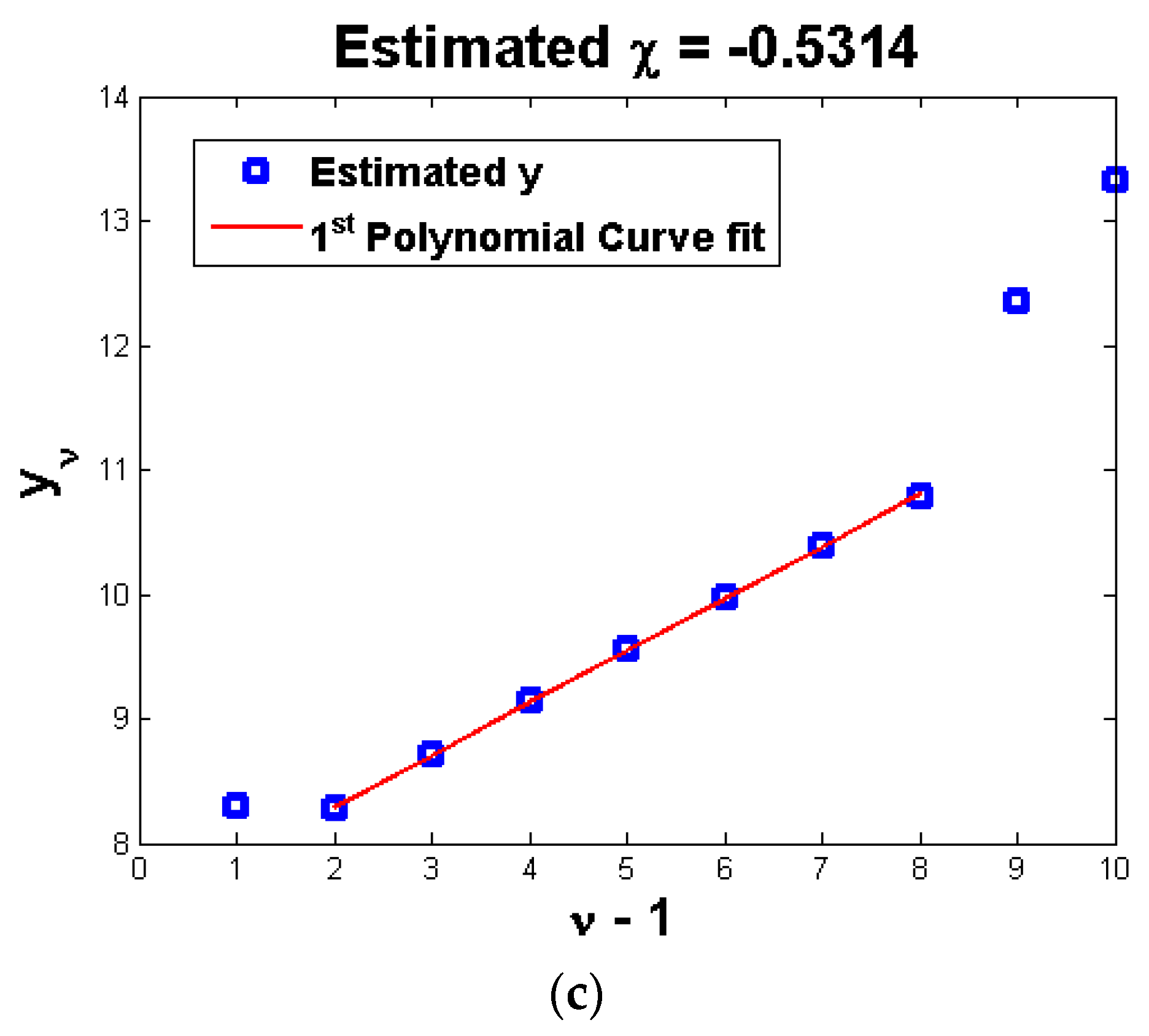
Equation (35) shows the difference in the damping values of sequential experiments in which the external force was increased z times in each trial. The results of this equation were obtained experimentally. If the results are plotted after taking the logarithmic function, which has z as the logarithm base, then the slope of this plot is $\chi +1$. Here, the abscissa indicated a negative one order for the performed experiments, and the ordinate indicated the measured values. This concept was similar to the conventional method used to estimate the value of $\chi$ by converting the dissipated energy with respect to the external harmonic force to a logarithmic scale. To estimate $\chi$ using Equation (35), linear curve fitting was performed on the measured damping values converted to a logarithmic scale. Here, the y intercept was regarded as $a_0$. Since z could be measured through experiments or as the magnitude ratio of the applied force in successive experiments, $\left|{\kappa }_1\right|B$ was estimated through a₀ in Equation (35). This was the same as $\Delta c_{l0}$ in Equation (33). As a result, every $\Delta c_{lv}$ in Equation (33) could be estimated.

By combining Equations. (33), (34), and (A15), the following relations were obtained:

$$R=\frac{\pi }{4}\frac{\left(\chi +2\right)\left(\chi +3\right)}{\left(z^{\left(\chi +1\right)}-1\right)}\frac{\Delta d_{l1}}{B}=\frac{\pi }{4}\frac{\left(\chi +2\right)\left(\chi +3\right)}{z^{\left(\chi +1\right)}\left(z^{\left(\chi +1\right)}-1\right)}\frac{\Delta d_{l2}}{B}=\cdots =\frac{\pi }{4}\frac{\left(\chi +2\right)\left(\chi +3\right)}{z^{\left(v-1\right)\left(\chi +1\right)}\left(z^{\left(\chi +1\right)}-1\right)}\frac{\Delta d_{lv}}{B}$$

(36)

In Equation (36), all of the variables except the constant B could be estimated by experiments. If a numerical model for the full system exists, then the stiffness $\mathit{K}$ in Equations (24) and (25) can be estimated, which was the case for the absence of joint components. If an experiment was performed by applying a very small force to the built-up structure, which includes the joint component, then the added stiffness ${\mathit{K}}_T$ at the interface could be estimated. Eventually, a static stiffness ${\mathit{K}}_J$ could be obtained. From this result, the mode shape for an undamped system could be estimated. In addition, if the external forces used in the experiments were applied to the numerical model to obtain the results in Equation (33), then the relative displacement at the contact surface could be estimated. Using these results, Equation (36) was re-arranged:

$$\tilde{R}=\frac{\pi }{4}\frac{\left(\chi +2\right)\left(\chi +3\right)}{\left(z^{\left(\chi +1\right)}-1\right)}\frac{\Delta d_{l1}}{\tilde{B}}=\frac{\pi }{4}\frac{\left(\chi +2\right)\left(\chi +3\right)}{z^{\left(\chi +1\right)}\left(z^{\left(\chi +1\right)}-1\right)}\frac{\Delta d_{l2}}{\tilde{B}}=\cdots =\frac{\pi }{4}\frac{\left(\chi +2\right)\left(\chi +3\right)}{z^{\left(v-1\right)\left(\chi +1\right)}\left(z^{\left(\chi +1\right)}-1\right)}\frac{\Delta d_{lv}}{\tilde{B}}$$

(37)

where $\tilde{B}={\displaystyle {\displaystyle \sum }_{m=1}^M}{P}_m({\tilde{\mathsf{\phi }}}_l){\tilde{A}}_{m_0}^{\chi +1}$.

The superscript tilde in Equation (37) indicates estimated values from the numerical model. This equation indicates that if $\tilde{B}$ was estimated using the mode shape and the relative displacements at the contact surface, which were obtained from the numerical model, then the parameter $\tilde{R}$ could be estimated.

3. Simulation

Degree-of-Freedom (DOF) Lumped Model

In this section, a simulation is conducted to verify the proposed method from the previous section. Figure 3 shows the configuration of the 10 DOF lumped model that is used in the simulation. Here, m and k represent the lumped mass and stiffness, respectively. In addition, u represents the displacement of each mass. As shown in the figure, two numbers of the Iwan model are assigned (one is connected between m₁ and m₆ and another is connected between m₂ and m₇). These two models show their dynamic characteristics according to the relative displacement of the connected nodes in the u direction. The frequency response function for this system is obtained by applying a force f at the lumped mass m₅, and we define the step sine as the applied force. In addition, a total of twelve experiments were conducted in this simulation, and in each experiment, the magnitude of the applied force follows the step sine, which increases consistently. Detailed introductions and specifications on the system and the performed experiments are as follows:

$$\begin{gathered} m_1=m_2=\cdots =m_{10}=1 \\ {k}_1=k_6=1.5\times {\mathrm{e}}^6,k_2=k_3=\cdots =k_5=k_7=\cdots =k_{10}=1\times {\mathrm{e}}^6 \\ {k}_{11}=0.3{\mathrm{e}}^6 ,k_{12}=0.5 \times {\mathrm{e}}^6 \\ f=2\times \left[2^0{2}^1{2}^2{2}^3\cdots 2^{11}\right] \end{gathered}$$

(38)

The four parameters on Iwan model include the following:

$$K_T=1.1e5,F_s=400,\chi =-0.5,\beta =4$$

(39)

Moreover, damping is assigned to increase the accuracy of the measurements made by the simulation. Proportional damping of the mass and stiffness matrices is assumed. As mentioned in the previous section, the stiffness matrix involved in this proportional damping is related to the stiffness K_J introduced in Equation (25):

$$C=aM+b{K}_J$$

(40)

In Equation (40), a and b are constants, and in this study, values of 5 × e⁻¹ and 7 × e⁻⁵ are assigned as these constants, respectively. In addition, the frequency resolution in the step sine experiment is 0.5 Hz and the time integral in the simulation is performed by the Newmark method [18].

Figure 4 shows the obtained FRFs from performed simulations. As shown in this figure, it can be confirmed that each mode has a different effect with respect to the magnitude of the external force. For instance, some modes (i.e., 2^nd, 4^th, 6^th and 8^th modes) show that their natural frequencies are shifted and that their peak values are decreased according to the increased magnitude of the force, whereas the other modes (i.e., 1^st, 3^rd, 5^th, 7^th and 9^th modes) hardly change their natural frequencies or their peak values. This is because the effect of the Iwan model is activated when relative displacement occurs in the region of interest. However, the modes that show no variations in the FRF results with respect to the changes of the external force all have in-phase motion in the interface between the masses of the Iwan model. The results shown in this figure are consistent to the statements in Ref. [13]. In addition, this figure magnifies the results for the 2^nd, 4^th and 6^th modes where variations in the frequency results occur with respect to the magnitude of the external force. From these magnified plots, changes of damping and the natural frequency can be identified in each experiment. To identify the parameter χ with the proposed method in this study, the results of Equation (35) for these three modes have been identified. In this process, the modal parameters for these modes have to be estimated. Recently, polyreference least-squares complex frequency-domain method which is so-called PolyMAX [19] is introduced as a modal parameter estimation method conducted in the frequency domain. It is one of the experimental modal parameter estimation methods and it guarantees stable identification of the system poles and participation factors. PolyMAX is applied to these three modes.

Figure 5 shows the results of Equation (35) for the three modes (□) obtained from the twelve experiments that were performed. In this figure, three plots are included as Figure 5a–c. These plots show the results for the selected modes. Among the results for each mode shown in this figure, a certain set is selected, which shows a constant increase of y values in each experiment. First degree polynomial curve fitting (—) has been applied on the selected data set in each mode, as shown in the figure. The parameter χ is estimated from the slope obtained by the curve fitting. The estimated results of χ are −0.528, −0.526 and −0.531 for the 2^nd, 4^th and 6^th mode, respectively. These results show approximately 5.2~6.5% error compared to the value defined for the system in Figure 3 (−0.5). In Figure 5b,c, there are no values defined in the range of y (□) from a value of zero (i.e., ν − 1 = 0) to the other end of the function domain. This is because the variation of damping, which is obtained from the first and second experiments, is too small to sense its value. Therefore, the variation cannot be represented by a logarithmic scale. In addition, in Figure 5c, this causes the similarity of values between 1 and 2 in the function domain. This is because the vibration magnitude at the higher modes (i.e., 4^th, 6^th modes) decreased compared to the lower mode (i.e., 2^nd mode). We performed other experiments to investigate the results in Figure 5 in more detail. PolyMAX was used to estimate the modal parameters of the twelve performed experiments. We have harmonically excited the system to the estimated natural frequency in each experiment with the same amplitude of force that was used in the twelve performed experiments at the same positions. Relative displacements are confirmed with respect to these excitations at the nodes where the Iwan model is connected (i.e., the relative displacement between m₁ and m₆, and the relative displacement between m₂ and m₇). These results are listed in

Table 1. List of the relative displacements in the Iwan models for the modes of interest.

Order of Exps.	2nd Mode		4th Mode		6th Mode
	Iwan1	Iwan2	Iwan1	Iwan2	Iwan1	Iwan2
1	0.00005	0.00016	0.00001	0.00003	0.00001	0.00001
2	0.00010	0.00030	0.00003	0.00006	0.00002	0.00002
3	0.00018	0.00057	0.00005	0.00011	0.00004	0.00004
4	0.00034	0.00106	0.00010	0.00021	0.00007	0.00007
5	0.00061	0.00191	0.00019	0.00041	0.00015	0.00013
6	0.00107	0.00337	0.00037	0.00078	0.00028	0.00025
7	0.00149	0.00471	0.00069	0.00146	0.00053	0.00048
8	0.00193	0.00592	0.00127	0.00268	0.00098	0.00089
9	0.00275	0.00855	0.00214	0.00451	0.00179	0.00162
10	0.00439	0.01372	0.00284	0.00601	0.00322	0.00291
11	0.00791	0.02345	0.00447	0.00935	0.00486	0.00455
12	0.01467	0.04335	0.00720	0.01493	0.00691	0.00658

.

Table 1 lists half of the peak to peak values of the measurements, which are measured in the time domain one second after a long period of time (i.e., 9 seconds was used in this study). The results in the table can be associated with the parameter ${\phi }_{max}$ of the Iwan model. ${\phi }_{max}$ can be obtained by the following relation [12] with the defined parameters in Equation (39):

$${\phi }_{\max }=\frac{F_s\left(1+\beta \right)}{K_T\left(\beta +\frac{\chi +1}{\chi +2}\right)}$$

(41)

The obtained ${\phi }_{max}$ from Equation (41) for the defined Iwan model in Equation (39) is 0.0042. From the results in the table, it can be confirmed that for the second mode in the second Iwan model of the seventh experiment (i.e., the relative displacement between m₂ and m₇), a larger value is obtained compared to the value of ${\phi }_{max}$ (0.0042) for the first experiment. This suggests that the macro-slip occurs in the seventh experiment for the first time. This also indicates that the system remained in the micro-slip region through the sixth experiment. The sixth experiment is associated with the 4 (ν-1) in the function domain in Figure 5. Therefore, in Figure 5a, the constant increase continues until function domain 4, but it shows abrupt changes at function domain 5. The same trend is confirmed in results of other modes. In the previous section, it was assumed that if one increases the amplitude of the external force as z times, then the relative displacement will linearly increase by z times. As confirmed in Table 1, however, it is observed that the results are less than z times (in this study, 2 times). The results of the estimated slope of the curve shown in Figure 5 show lower values than the true value.

Eventually, this results in a larger amplitude (0.52~0.53) of the estimated χ than the true value.

Next, R is estimated using the estimated χ and Equation (37), as shown in Figure 5. Similar to ${\phi }_{max}$, R can be obtained with the defined parameters in Equation (39) by the following relation which is introduced in Reference [12].

$$R=\frac{F_s\left(\chi +1\right)}{{\phi }_{\max }^{\chi +2}\left(\beta +\frac{\chi +1}{\chi +2}\right)}$$

(42)

The obtained R by Equation (42) is 1.69 × e⁵. In this study, the constant $\tilde{B}$ in Equation (37) was obtained in two different ways. First, relative displacements that are necessary to estimate this constant are obtained by the same way that is introduced in the previous section. This indicates that the system matrices M, C, and K_J are obtained and estimate the relative displacements at nodes associated with the Iwan model by solving the inverse problem with these matrices. Then, $\tilde{R}$ can be estimated by using the estimated $\tilde{B}$ and Equation (37). The errors between the estimated $\tilde{R}$ and the obtained true value of R by Equation (42) are listed in

Table 2. List of the errors of the estimated $\tilde{R}$ compared to the obtained R.

ν-1	2nd Mode		4th Mode		6th Mode
	Inverse Matrix (%)	Newmark Method (%)	Inverse Matrix (%)	Newmark Method (%)	Inverse Matrix (%)	Newmark Method (%)
0	13.199	10.574	31.887	15.272	100.000	100.000
1	9.937	7.214	28.839	12.608	135.950	37.369
2	8.675	5.913	28.704	12.490	67.009	2.768
3	10.367	7.656	22.844	7.368	67.679	2.379
4	18.818	16.363	22.321	6.911	68.544	1.875
5	117.323	123.895	21.789	6.446	64.167	4.423
6	217.785	227.395	20.967	5.727	61.796	5.804
7	169.117	177.255	59.959	39.806	58.587	7.672
8	63.680	68.630	295.122	245.344	54.384	10.119
9	69.430	68.505	306.771	255.524	239.717	97.781
10	132.867	133.861	292.655	243.187	385.652	182.743

in percent format (%).

In Table 2, the inverse matrix shows the obtained results using the method proposed in this study with relative displacement, whereas the Newmark methods results are given in Table 1. If one examines the characteristics observed in this table, the same region corresponding to the linear region where the curve fitting process was performed in Figure 5 can confirm that the results in the table show more closed values than the true value of the defined R. In addition, the results, which were estimated using the results in Table 1 (Newmark method), are more accurate than the estimated results using the proposed method (Inverse matrix). Furthermore, as the mode number increases, the error of the estimated results of the proposed method also increases. This result is related to the mode shape because the estimated mode shape ${\mathit{\phi }}_n$ from the lumped model is different to the true mode shape in dynamic behavior. Based on the results in the table, the difference between these two mode shapes (i.e., the lumped model vs. practical behavior) increases as the mode number increases.

4. Experiments

Experiments were performed on a partially connected double beam in order to verify the proposed method in Section 2. Figure 6 shows the double layer beam, which was composed of two identical aluminum cantilever beams (350 mm × 50 mm × 1 mm) with one end clamped and the other end fixed with glue. The glue was evenly distributed along the longitudinal direction of the beam for 20 mm. As shown in the figure, the exciter was located on the clamped side and the force transducer was located between the exciter and the double beam system. The vibration induced by the exciter was measured with an accelerometer, which was located in same position as the accelerator (Acc. 1).

In order to verify the proposed method, several experiments were conducted, as introduced in the theory section. Experiments were performed while increasing the voltage applied to the exciter twice. In these experiments, a linear relationship between the force and the applied voltage was assumed. The linear relationship was confirmed by attaching accelerometers to the area where the beams were glued. In the figure, the magnitude of the relative acceleration measured by Acc. 2 and Acc. 3 doubled in successive experiments. Thus, there was a linear relationship between the applied force and the voltage. The experiment was performed ten times from 5 mV to 2.56 V. The excitation frequency varied from 50 to 450 Hz based on the reliability of the exciter and the step sine used 2 Hz intervals.

Figure 7 shows the FRFs measured in the 10 experiments performed. The second mode in the figure shows that the peak values at the resonance frequency decreased as the applied force increased. That is, the mode shape at the contact region was predominantly governed by the slip phenomenon by out-of-mode shape. Other modes were independent to the magnitude of the external force. Typically, this tendency is confirmed by the peak value in the fifth mode. In order to estimate the variation of natural frequencies and damping ratios in response to a change in external force, the two parameters of the Iwan model were estimated. The proposed method was applied to the measurements from the first seven experiments. The natural frequencies and damping ratios of the remaining three experiments were predicted using the estimated two parameters. The modal parameters, natural frequency, and damping ratio, predicted using the estimated two parameters from the remaining three experiments, were compared with the estimated modal parameters from the real measurements of the same experiments. First, Equation (35) was applied to the second mode in the figure.

The resultant y_v values showed a large deviation at a small force level and a nearly linear trend where the force was increased. This was because slip rarely occurs when the external force is small, and in this case, the estimated results by the proposed method were more sensitive to the noise in the experiment. This tendency was also confirmed in the simulation results. The objective $\chi$ was estimated using the damping ratios calculated from the first seven experiments. Figure 8 represents the difference in energy dissipation in successive experiments; thus, $\chi$ was estimated by curve fitting the first six results by a 1^st order straight line (—). The estimated result was −0.37366. Next, the parameter R of the Iwan model was estimated using Equation (37), but first the mode shape of the partially connected double beam shown in Figure 6 had to be determined. The mode shape of a partially connected double beam was studied analytically and numerically in [20]. By applying Equation (37) to the mode shape vector, R was estimated as 3.5431 × e⁺⁵. Utilizing the estimated $\chi$ and R, the natural frequencies and damping ratios were estimated using the measurements in the 8^th, 9^th, and 10^th experiments. The variation of natural frequency, $\Delta {\omega }_n^2$, when increasing the external force is represented in Equation (30). It can also be represented as follows, similar to Equation (33):

$$\begin{gathered} \Delta {\omega }_{l0}^2={\kappa }_2{\displaystyle \sum }_{m=1}^M{P}_m\left({\mathit{\phi }}_l\right)A_{m_0}^{\chi +1}={\kappa }_{2}B \\ \Delta {\omega }_{l1}^2={\kappa }_2{\displaystyle \sum }_{m=1}^M{P}_m\left({\mathit{\phi }}_l\right){\left(z{A}_{m_0}\right)}^{\chi +1}=z^{\left(\chi +1\right)}{\kappa }_{2}B \\ \Delta {\omega }_{l2}^2={\kappa }_2{\displaystyle \sum }_{m=1}^M{P}_m\left({\mathit{\phi }}_l\right){\left(z^2{A}_{m_0}\right)}^{\chi +1}=z^{2\left(\chi +1\right)}{\kappa }_{2}B \\ \Delta {\omega }_{l3}^2={\kappa }_2{\displaystyle \sum }_{m=1}^M{P}_m\left({\mathit{\phi }}_l\right){\left(z^3{A}_{m_0}\right)}^{\chi +1}=z^{3\left(\chi +1\right)}{\kappa }_{2}B \\ ⋮ \\ \Delta {\omega }_{lv}^2={\kappa }_2{\displaystyle \sum }_{m=1}^M{P}_m\left({\mathit{\phi }}_l\right){\left(z^v{A}_{m_0}\right)}^{\chi +1}=z^{v\left(\chi +1\right)}{\kappa }_{2}B \end{gathered}$$

(43)

where $B={{\displaystyle \sum }}_{m=1}^M{P}_m\left({\mathit{\phi }}_l\right)A_{m_0}^{\chi +1}.$ Using the y-intercept in Figure 8 and Equation (35), $\left|{\kappa }_1\right|B$ was found to be 29.431. By substituting the estimated $\chi$ and R into Equation (A15), ${\kappa }_1$ was obtained. Utilizing the estimated value and $\left|{\kappa }_1\right|B$, the following result was determined: $B=2.787$ × e⁻⁴. Additionally, ${\kappa }_2$ was found using Equations. (A12) and (A15). $\Delta {\omega }_n^2$, which represents the change in natural frequency, could then be obtained for the 8^th through 10^th experiments. Based on obtained $\Delta {\omega }_n^2$, the natural frequency ${\omega }_n^2$ was estimated.

The second column of

Table 3. List of $\Delta {\omega }_n^2$ between successive experiments.

Order of Expt.	Measured (rad2/sec2)	Estimated (rad2/sec2)	Error (%)
1st to 2nd	8.18	*	*
2nd to 3rd	40.45	*	*
3rd to 4th	−23.11	*	*
4th to 5th	39.92	*	*
5th to 6th	59.58	*	*
6th to 7th	148.04	*	*
7th to 8th	114.08	110.71	−2.94
8th to 9th	206.67	180.91	−12.47
9th to 10th	304.64	283.82	−6.83

is the variation in the natural frequencies $\Delta {\omega }_n^2$ between successive experiments. The third column shows the variation of the natural frequencies estimated by applying the proposed method, Equation (43), to the experimental results from the first to the seventh trials. The fourth column shows the error between the experimental and estimated values. On average, the error was less than 10%.

Table 4. List of ${\omega }_n^2$ in every experiment.

Order of Expt.	Measured (rad2/sec2)	Estimated (rad2/sec2)	Error (%)
1st	2.50677 × e6	*	*
2nd	2.50676 × e6	*	*
3rd	2.50672 × e6	*	*
4th	2.50674 × e6	*	*
5th	2.50670 × e6	*	*
6th	2.50671 × e6	*	*
7th	2.50656 × e6	*	*
8th	2.50645 × e6	2.50646 × e6	4 × e−4
9th	2.50624 × e6	2.50641E × e6	6.5 × e−3
10th	2.50594 × e6	2.50631 × e6	1.5 × e−2

shows the natural frequencies ${\omega }_n^2$ for the individual experiments, as obtained through Table 3. The second column is the measured ${\omega }_n^2$ in the experiment and the third column is the result estimated from Table 4. The fourth column shows the error between the experimental and the estimated values. Since the natural frequency is large, even if there was an error of 10% in the variation of the natural frequency listed in Table 3, the estimated natural frequency was very accurate at an error of less than 0.1%. $\Delta {\omega }_n^2$ in the denominator of Equation (31) was directly related to the variation in natural frequencies measured experimentally. However, the relation between $\Delta c_n$ and the damping ratio ${\zeta }_J$ measured through the experiment should be confirmed. The denominator of the FRF for the individual modes in the modal domain, as derived from the equations of motion for the linear structure is:

$$\left({\omega }_J^2-{\omega }^2\right)+j2{\zeta }_J{\omega }_J\omega$$

(44)

In Equation (44), ${\omega }_J$ and ${\zeta }_J$ denote the natural frequencies and damping ratios measured, respectively, by applying the experimental modal analysis method to the experiments. Through the imaginary part of Equations (31) and (44), $\Delta c_n$ and ${\zeta }_J$ have the following relation.

$${\zeta }_J={\zeta }_n\frac{{\omega }_n}{{\omega }_J}+\frac{\Delta c_n}{{\omega }_J^2}\cong {\zeta }_n+\frac{\Delta c_n}{{\omega }_J^2}$$

(45)

In Equation (45), ${\omega }_n$ and ${\zeta }_n$ are the natural frequency and damping ratio of the structure, respectively, when there is no Iwan model in the structure or when the structure vibrates with very small forces. Assuming that the ratio of ${\omega }_J$ and ${\omega }_n$ is close to one, the damping ratio measured from the experiment is expressed as the right-hand side of Equation (45). From Equation (33), $\Delta c_{l0}=\left|{\kappa }_1\right|B$; thus, every $\Delta c_{lv}$ in Equation (33) can be determined. ${\omega }_J$ and ${\zeta }_J$ were measured through experiments and $\Delta c_n$ was predicted through the proposed method.

$$\Delta {\zeta }_{Jv}={\zeta }_{Jv}-{\zeta }_{Jv-1}\cong \frac{\Delta c_{nv}}{{\omega }_{Jv}^2}-\frac{\Delta c_{nv-1}}{{\omega }_{Jv-1}^2}$$

(46)

Equation (46) was derived from Equation (45) and shows the damping ratio change when the external force increases. Subscript J is the damping ratio measured in the experiment, and subscript v is the index of the experiment performed with increasing force level. As a result, the damping ratio measured from the 8^th through 10^th experiments could be estimated from Equation (46).

The second column of

Table 5. List of $\Delta {\zeta }_{Jv}$ between successive experiments.

Order of Expt.	Measured (%)	Estimated (%)	Error (%)
1st to 2nd	6.072 × e−4	*	*
2nd to 3rd	−4.385 × e−4	*	*
3rd to 4th	2.457 × e−4	*	*
4th to 5th	1.167 × e−3	*	*
5th to 6th	2.118 × e−3	*	*
6th to 7th	3.804 × e−3	*	*
7th to 8th	4.122 × e−3	4.012 × e−3	−2.67
8th to 9th	5.569 × e−3	5.329 × e−3	−4.30
9th to 10th	9.583 × e−3	8.280 × e−3	−13.60

is the variation of damping ratio $\Delta {\zeta }_{Jv}$ between consecutive experiments and the third column is the variation of the estimated damping ratio when applying the proposed method to the experimental results of the first seven experiments. The fourth column shows the error between the experimental and estimated values. The overall average error was less than 7%.

Table 6. List of ${\zeta }_{Jv}$.

Order of Expt.	Measured (%)	Estimated (%)	Error (%)
1st	1.2780	*	*
2nd	1.2795	*	*
3rd	1.2791	*	*
4th	1.2793	*	*
5th	1.2805	*	*
6th	1.2830	*	*
7th	1.2864	*	*
8th	1.2905	1.2888	−1.3 × e−1
9th	1.2961	1.2940	−1.6 × e−1
10th	1.3056	1.3021	−2.7 × e−1

shows the damping ratios for individual experiments estimated based on Table 5. The second column was measured in the experiment and the third column is from Table 5. The fourth column shows the error between the experimental value and the estimated value. Since the damping ratio was larger than the variation in the damping ratio, the estimated damping ratio guaranteed a very accurate estimate with an error of less than 1%. This held even if the variation of the damping ratio estimated in Table 5 was 7%. Through the experiments performed, the estimation of variations in the natural frequency and the damping ratio had an error of 10% compared with the actual measurements. The natural frequencies and damping ratios; however, estimated based on the estimated variations were confirmed to be very accurate with less than 1% error. The reliability and effectiveness of the proposed method were, thus, verified.

5. Summary and Conclusions

Many studies have reported the change of dynamic characteristics of built-up structures with an increase in internal energy. Previous studies used the Iwan model to investigate the change of dynamic characteristics by the slip phenomenon on the contact interface. In general, the Iwan model consists of four parameters {χ, K_T, F_S, and β}, where {χ and K_T} represent the change of dynamic characteristics in the micro-slip regime, and {F_S and β} determine the characteristics at the border line of the micro- and macro-slip regimes. In this study, it is assumed that built-up structures vibrate only in the micro-slip regime. To estimate the two parameters that determine the dynamic characteristics in the micro-slip regime, modal analysis is done instead of quasi-static experiments, which were used in the previous studies. Further, modal equations for each mode of the built-up structures were derived. A technique to estimate two parameters using the derived modal equations was proposed.

In this study, to estimate the variation of natural frequency and damping ratio according to the change in internal energy or external force, the slip phenomenon occurring at the built-up structure’s interface was described using the Iwan model. Based on this model, the variation of natural frequency and damping ratio were estimated. The proposed method was developed and tested to estimate two out of the four parameters, which define the Iwan model. The study used modal analysis. In this process, the force variation occurring in the constitutive model during dynamic behavior was investigated. The numerical model for the full system was examined. In addition, the numerical model and modal analysis were combined to determine a method that could estimate the parameters using variations in the damping magnitude. This proposed method was verified through simulations. The characteristics of the results were examined. To verify the proposed method, 10 experiments were performed using a partially connected double beam structure with increasing external force. Two parameters of the Iwan model were estimated by applying the proposed method to the first seven experiments. The estimated parameters were then used to determine the dynamic characteristics for the remaining three experiments. We could, thus, confirm the reliability of the proposed method.

References

1. Chung, J.S.; Whitney, A.K.; Loden, W.A. Nonlinear Transient Motion of Deep Ocean Mining Pipe. J. Energy Resour. Technol. 1981, 103, 2–10. [Google Scholar] [CrossRef]
2. Gordis, J.H.; Radwick, J. Efficient transient analysis for large locally nonlinear structures. Shock Vibr. 1999, 6, 1–9. [Google Scholar] [CrossRef]
3. Nayfeh, H. Nonlinear Oscillations; WILEY-VCH Verlag GmbH & CO. KGaA: Weinheim, Germany, 2007. [Google Scholar]
4. Reddy, J.N. Geometrically nonlinear transient analysis of laminated composite plates. AIAA J. 1984, 21, 621–629. [Google Scholar] [CrossRef]
5. Lee, J.; Wang, S.; Kindt, P.; Pluymers, B.; Desmet, W. Damping analysis with respect to rolling speed by analytic solution of a flexible ring model and its frequency response function derivation by modal summation method. Int. J. Appl. Mech. 2014, 6, 1450054. [Google Scholar] [CrossRef]
6. Al-Mayah, A.; Moseley, J.; Brock, K.K. Contact surface and material nonlinearity modeling of human lungs. Phys. Med. Biol. 2008, 53, 305. [Google Scholar] [CrossRef] [PubMed]
7. Dahl, P.R. Solid friction damping of mechanical vibrations. AIAA J. 1976, 14, 1675–1682. [Google Scholar] [CrossRef]
8. Marhefka, D.W.; Orin, D.E. A compliant contact model with nonlnear damping for simulations of robotic systems. IEEE Trans. Syst. ManCybern. Part A Syst. Hum. 1999, 29, 566–572. [Google Scholar] [CrossRef]
9. Iwan, W.D. A distributed-element model for hysteresis and its steady-state dynamic response. ASME J. Appl. Mech. 1966, 33, 893–900. [Google Scholar] [CrossRef]
10. Iwan, W.D. On a class of models for the yielding behavior of continuous and composite systems. ASME J. Appl. Mech. 1967, 34, 612–617. [Google Scholar] [CrossRef]
11. Segalman, D.J. An Initial Overview of Iwan Modeling for Mechancal Joints; Report No. SAND2001-0811; Sandia National Laboratories: Albuquerque, NM, USA, 2001.
12. Segalman, D.J. A four-parameter Iwan model for lap-type joints. ASME J. Appl. Mech. 2005, 72, 752–760. [Google Scholar] [CrossRef]
13. Segalman, D.J. A Modal Approach to Modeling Spatially Distriubted Vibration Energy Dissipation; Report No. SAND2010-4760; Sandial National Laboratories: Albuquerque, NM, USA, 2010.
14. He, K.; Zhu, W.D. Finite element modeling of structures with L-shaped beams and bolted joints. J. Vib. Acoust. ASME 2011, 133, 011011. [Google Scholar] [CrossRef]
15. Sanati, M.; Terashima, Y.; Shamoto, E.; Park, S.S. Development of a new method for joint damping identification in a bolted lap joint. J. Mech. Sci. Technol. 2018, 32, 1975–1983. [Google Scholar] [CrossRef]
16. Li, Y.; Hao, Z.; Feng, J.; Zhang, D. Investigation into discretization methods of the six-parameterIwan model. Mech. Syst. Signal Process. 2017, 85, 98–110. [Google Scholar] [CrossRef]
17. Berger, E. Friction modeling for dynamic system simulation. Appl. Mech. Rev. 2002, 55, 535–577. [Google Scholar] [CrossRef] [Green Version]
18. Newmark, N.M. A method of computation for structural dynamics. J. Eng. Mech. Div. 1959, 85, 67–94. [Google Scholar]
19. Heylen, W.; Lammens, S.; Sas, P. Modal Analysis Theory and Testing; KU Leuven—PMA: Leuven, Belgium, 1998. [Google Scholar]
20. Lee, J.; Wang, S. Vibration analysis of a partially connected double-beam system with the transfer matrix method and identification of the slap phenomenon in the system. Int. J. Appl. Mech. 2017, 9, 1750093. [Google Scholar] [CrossRef]
Figure 1. Description of the parallel-series Iwan model.
Applsci 09 04290 g001
Figure 2. Description of the 2 DOF system connected by the stiffness k and the Iwan model between the ith and jth nodes.
Applsci 09 04290 g002
Figure 3. Description of the 10 DOF system with two numbers of the Iwan model.
Applsci 09 04290 g003
Figure 4. Numerically obtained twelve number of frequency response functions with respect to step sine excitations.
Applsci 09 04290 g004
Figure 5. Estimated y in Equation (35) (), results of curve fit with 1st polynomial equation () and estimated results of χ from the curve fitting results: (a) for 2nd mode, (b) for 4th mode, (c) for 6th mode.
Applsci 09 04290 g005aApplsci 09 04290 g005b
Figure 6. Experimental configuration.
Applsci 09 04290 g006
Figure 7. Measured frequency response functions.
Applsci 09 04290 g007
Figure 8. Estimated y in Equation (35) (), results of curve fit with 1st polynomial equation () and estimated χ from the curve fitting results.
Applsci 09 04290 g008