Monin–Obukhov Similarity Theory for Modeling of Wind Turbine Wakes under Atmospheric Stable Conditions: Breakdown and Modifications

Abstract

Monin–Obukhov similarity theory (MOST) overestimates the mean vertical velocity gradient in some atmospheric stable conditions, i.e., Richardson number $R_f<0.25$. To obtain a given hub-height inflow velocity for a certain roughness length, this overestimated velocity gradient underpredicts the friction wind speed and the turbulence intensity, potentially influencing wake modeling of a wind turbine. This work investigates the side effects of the breakdown of MOST on wake modeling under stable conditions and makes some modifications to the flow similarity functions to eliminate these side effects. Based on a field measurement in a wind farm, we first show that MOST predicts a larger velocity gradient for the atmospheric stability parameter $\zeta >0.1$ and proposes new flow similarity functions without constraining $R_f$ to limit the overestimated velocity gradient. Next, different turbulence models based on MOST and a modified one based on the new similarity functions are investigated through numerical simulations. These turbulence models are combined with the actuator disk model (AD) and Reynolds-averaged Navier–Stokes equations (RANS) to model wind turbine wakes under stable conditions. As compared to measurements, numerical results show that turbulence models based on MOST result in a larger wake deficit and a slower wake recovery rate with a root-mean-squared error (RSME) of wake deficit in the range of 0.07 to 0.20. This overestimated wake effect is improved by applying the new similarity functions, and the RSME of wake deficit is reduced by 0.05 on average.

1. Introduction

As a measure of turbulence exchanges in the atmospheric surface layer, atmospheric stability can significantly affect the wind turbine wake deficit and its recovery rate. In general, turbulence exchanges between the wake and atmosphere are depressed under stable conditions. High wake deficits and slow wake recovery, thus, are usually observed in the stable stratification boundary layer [1,2]. As wakes play critical roles in wind farm energy production and the fatigue loads of wind turbines, there is an increasing interest in studying the effects of atmospheric stability on wakes and developing wake models for non-neutral conditions.

The impact of atmospheric stability on wakes is widely observed in wind tunnel measurements of small-scale models of wind turbines [3,4,5] and full-scale field experiments [1,2,6,7,8]. According to the wind tunnel measurements in Chamorror et al. [3], the stronger inlet velocity gradient in the stable case leads to a slightly stronger turbulence intensity and extends the region of enhanced turbulence intensity from a distance of approximately 4 to 5.5 rotor diameters to 3 and 6 rotor diameters downwind of the turbine location. In Zhang et al. [4], a 15% smaller velocity deficit at the wake center, a more rapid momentum recovery due to an enhanced radial momentum transport, and 20% higher peak turbulence intensity were observed in the unstable case, as compared to the wake of the same wind turbine under neutral conditions. According to the field experiments of wakes using LiDARs or masts, Magnusson et al. [6], Iungo et al. [7], and Han et al. [2] also found that the velocity deficit decreases more slowly under stable conditions and more quickly under unstable conditions. Those observations suggest that atmospheric stability should be considered for improved wake models and predictions of wind power harvesting.

Besides field measurements and wind tunnel experiments of wind turbine wakes under non-neutral conditions, numerical models based on the computational fluid dynamics (CFD) have also been used to investigate the effect of atmospheric stability on the wind turbine wakes [1,9,10,11,12,13,14]. High-fidelity large eddy simulations (LES) with the actuator line model [9,10] or the actuator disk model [1,11] are commonly used to study the structure and dynamics of wind turbine wakes in varying stability cases. This is mainly because the LES approaches allow capturing the near wake structure and resolving the interactions of tip vortices with large-scale eddies of the ambient flow and wake meandering. However, the high-fidelity approaches are computationally expensive for wind energy engineering applications. There are some efforts towards developing turbulence models for wind turbine wakes under non-neutral conditions in reynolds-averaged navier–Stokes (RANS) to reduce computational costs.

A widely used turbulence model for the thermal stratified boundary layer was developed by Alinot and Masson [15], where a coefficient of the buoyant terms in the transport equation of the turbulence kinetic energy dissipation is calibrated with atmospheric stability. However, van der Laan et al. [16] showed that this model cannot keep the flow homogeneity in a large domain under unstable conditions and thus developed a turbulence model consistent with monin–obukhov similarity theory (MOST). In [13], an additional buoyancy production based on the Richardson number, $Ri$, was added to the turbulent kinetic energy equation to model wind turbine wakes under stable conditions. El-Askary et al. [14] further applied this model with an additionally dissipation source term to investigate the wake behavior at different atmospheric stability conditions. Note that these turbulence models are based on MOST and could fail in modeling wind turbine wakes when MOST breaks down under stable conditions for the flux Richardson number $R_f>0.25$. According to the literature [17,18], the classical similarity functions that are widely used in MOST to determine the wind profile are only valid for $R_f<0.25$ and overestimate the velocity gradient for $R_f>0.25$. For a given aerodynamic roughness $z_0$ and a hub-height inflow velocity, this overestimated velocity gradient results in a smaller friction wind speed $u_{*}$, and consequently a lower turbulence intensity, and could influence wake modeling of wind turbines.

To the best of our knowledge, the side effects of the breakdown of MOST on wake modeling under stable conditions have not been well investigated. The present paper aims to investigate these side effects through numerical simulations and to make a modification on MOST to eliminate these side effects. This modification proposes a new set of similarity functions based on field measurements to limit the velocity gradient in very stable conditions and introduce the new similarity functions into the turbulence model proposed by van der Laan et al. [16]. The remainder of this paper is organized as follows. MOST is briefly described in Section 2. Models for wind turbine wakes under stable conditions are introduced in Section 3, which cover two actuator disk models based on the thrust coefficient and Blade Element Theory (BEM) calculations, and three turbulence models for stable conditions based on MOST. Section 3 also proposes a modified turbulence model that can be consistent with arbitrary similarity functions, e.g., the new similarity functions. The breakdown of MOST under stable conditions is experimentally investigated and new similarity functions are proposed and validated in Section 4. All test models are studied through numerical simulations: the simulation details are described in Section 5, and the results of the simulations are discussed in Section 6 and then concluded in Section 7.

2. Monin–Obukhov Similarity Theory

According to MOST [19], any dimensionless characteristics of the turbulence depends only on the dimensionless stability parameter $\zeta =z/L$, where z is the height above the surface and the Obukhov length L that is defined by

$$L\equiv -\frac{u_{*}^3}{\kappa \frac{g}{\Theta }\overline{w^{\prime }{\theta }^{\prime }}}$$

(1)

in which $\kappa =0.4$, g is the gravity acceleration, $\Theta$ is the time-averaged potential temperature, ${\theta }^{\prime }$ is the fluctuation of the potential temperature, and $u_{*}=\sqrt{-\overline{u^{\prime }{w}^{\prime }}}$ is the friction speed, where $u^{\prime }$ and $w^{\prime }$ are the fluctuations of the longitudinal and vertical velocity components.

The flow similarity functions of the gradient of velocity, the gradient of potential temperature, the turbulence kinetic energy, and its dissipation can thus be defined as

$${\varphi }_m\left(\zeta \right)\equiv \frac{\kappa z}{u_{*}}\frac{\partial U}{\partial z}$$

(2)

$${\varphi }_h\left(\zeta \right)\equiv \frac{\kappa z}{{\theta }_{*}}\frac{\partial \Theta }{\partial z}$$

(3)

$${\varphi }_k\left(\zeta \right)\equiv \frac{\sqrt{C_{\mu }}}{u_{*}^2}k$$

(4)

$${\varphi }_{\epsilon }\left(\zeta \right)\equiv \frac{\kappa z}{u_{*}^3}\epsilon$$

(5)

where U is the mean streamwise speed, ${\theta }_{*}=-\overline{w^{\prime }{\theta }^{\prime }}/u_{*}$ is the scaling temperature, $C_{\mu }=0.033$, k is the turbulence kinetic energy (TKE), and $\epsilon$ is the TKE dissipation. According to the eddy viscosity hypothesis by Boussinesq [20], we have

$$-\rho \overline{u^{\prime }{w}^{\prime }}={\mu }_t\frac{\partial U}{\partial z}$$

(6)

where $\rho$ is the air density and the eddy viscosity is modeled in the $k-\epsilon$ model as [21]

$${\mu }_t=\rho C_{\mu }\frac{k^2}{\epsilon }$$

(7)

Combining the definitions of ${\varphi }_m,{\varphi }_k$, and ${\varphi }_{\epsilon }$ with Equations (6) and (7) leads to

$${\varphi }_k\left(\zeta \right)=\sqrt{({\varphi }_{\epsilon }\left(\zeta \right)/{\varphi }_m\left(\zeta \right)}$$

(8)

Based on measurements of flows over flat terrain in the atmospheric surface layer, the classical similarity functions commonly used in literature are given as [22,23]

$${\varphi }_{m,\mathrm{cls}}\left(\zeta \right)=\left\{\begin{array}{cc}{(1-{\gamma }_m\zeta )}^{-1/4}\hfill & -2<\zeta <0\hfill \\ 1+{\beta }_m\zeta \hfill & 0<\zeta <1\hfill \end{array}\right.$$

(9)

$${\varphi }_{h,\mathrm{cls}}\left(\zeta \right)=\left\{\begin{array}{cc}\chi {(1-{\gamma }_h\zeta )}^{-1/2}\hfill & -2<\zeta <0\hfill \\ \chi +{\beta }_h\zeta \hfill & 0<\zeta <1\hfill \end{array}\right.$$

(10)

$${\varphi }_{\epsilon ,\mathrm{cls}}\left(\zeta \right)=\left\{\begin{array}{cc}1-\zeta \hfill & \zeta <0\hfill \\ {\varphi }_{m,\mathrm{cls}}-\zeta \hfill & \zeta >0\hfill \end{array}\right.$$

(11)

where ${\gamma }_m={\gamma }_h=16$, ${\beta }_m={\beta }_h=5$ [23], and $\chi$ will be determined based on field measurements in Section 4. The classical similarity functions ${\varphi }_m$ and ${\varphi }_h$ are, however, only valid for the flux Richardson number $R_f$ below 0.25 [17]. We thus proposed new functions, noted as ${\varphi }_{m,\exp }$ and ${\varphi }_{h,\exp }$, in the full range of $R_f$ based on a field experiment in a wind farm.

3. Models for Wind Turbine Wakes under Stable Conditions

In the present work, the numerical simulation of wind turbine wakes under atmospheric stable conditions is based on RANS equations and the buoyancy effect due to atmospheric thermal stratifications is also taken into account. The following continuity, momentum, and energy equations are solved in wake simulations [15,24],

$$\frac{\partial }{\partial x_i}\left(\rho U_i\right)=0$$

(12)

$$\frac{\partial }{\partial t}\left(\rho U_i\right)+\frac{\partial }{\partial x_j}\left(\rho U_i{U}_j\right)=-\frac{\partial p}{\partial x_i}+\frac{\partial }{\partial x_j}\left[(\mu +{\mu }_t)\left(\frac{\partial U_i}{\partial x_j}+\frac{\partial U_j}{\partial x_i}\right)\right]+S_{u,i}$$

(13)

$$\frac{\partial }{\partial t}(\rho \Theta )+\frac{\partial }{\partial x_i}(\rho U_i\Theta )=\frac{\partial }{\partial x_i}\left[\left(\frac{\mu }{Pr}+{\alpha }_t\right)\frac{\partial \Theta }{\partial x_i}\right]$$

(14)

where $\rho$ is the air density, $U_i$ is the velocity component in the $x_i$ direction, p is the air pressure, $\mu$ is the laminar viscosity, ${\mu }_t$ is the turbulent viscosity, $S_{u,i}$ is the momentum term source imposed by the wind turbine rotor in the $x_i$ direction, $\Theta$ is the potential temperature, $Pr=0.9$ is the laminar Prandtl number, and ${\alpha }_t\equiv {\mu }_t/P{r}_t$ is the turbulent heat conductivity, where $P{r}_t$ is the turbulent Prandtl number.

3.1. Modeling of Wind Turbine

In this work, we introduce two kinds of actuator disk models: one is based on the thrust coefficient and another is based on BEM calculations to distribute forces through the disk. The second model, which provides more detailed information of the distributed forces caused by the rotor, is expected to capture near wake structure better than the first one. All simulations carried out in this work use the AD model based on BEM calculations in advance if the geometry information of the blades is available.

3.1.1. Actuator Disk Model Based on Thrust Coefficient (-CT)

In the origin actuator disk model, the momentum source term in the $x_i$ direction due to the thrust is uniformly distributed through the rotor:

$$S_{u,i}=-\frac{T}{V_{\mathrm{disk}}}\frac{U_{\mathrm{ref},i}}{U_{\mathrm{ref}}}=-\frac{\rho C_T{U}_{\mathrm{ref}}{U}_{\mathrm{ref},i}}{2\Delta l}$$

(15)

where T is the thrust, $V_{\mathrm{disk}}$ is the disk volume, $C_T$ is the thrust coefficient, $U_{\mathrm{ref}}$ is the upstream reference velocity at hub height, $U_{\mathrm{ref},i}$ is the component velocity $U_{\mathrm{ref}}$ of in $x_i$ direction, $\Delta l$ is the disk depth, and the negative sign represents the drag effects of thrust on the flow.

For the upstream flow disturbed by a complex terrain or wind turbine wakes, $U_{\mathrm{ref}}$ is unknown and difficult to evaluate from the local flow directly. According to the one-dimensional momentum theory and ignoring the velocity gradient, the reference velocity is a function of the rotor-averaged velocity $U_{\mathrm{disk}}$:

$$U_{\mathrm{disk}}=(1-a_B)U_{\mathrm{ref}}$$

(16)

in which the induced factor $a_B$ [25] is related to the thrust coefficient $C_T$ by

$$a_B=\left\{\begin{array}{cc}\frac{1}{2}(1-\sqrt{1-C_T}),\hfill & C_T\le \frac{8}{9}\hfill \\ \frac{C_T-4a_c^2}{4(1-2a_c)},\hfill & C_T>\frac{8}{9}\hfill \end{array}\right.$$

(17)

where $a_c=1/3$.

In simulations, the disk-averaged velocity $U_{\mathrm{disk}}$ is calculated by averaging the local velocity in the disk region, then is applied to estimate the upstream reference velocity $U_{\mathrm{ref}}$ based on Equations (16) and (17) and the momentum source $S_{u,i}$ based on Equation (15), respectively.

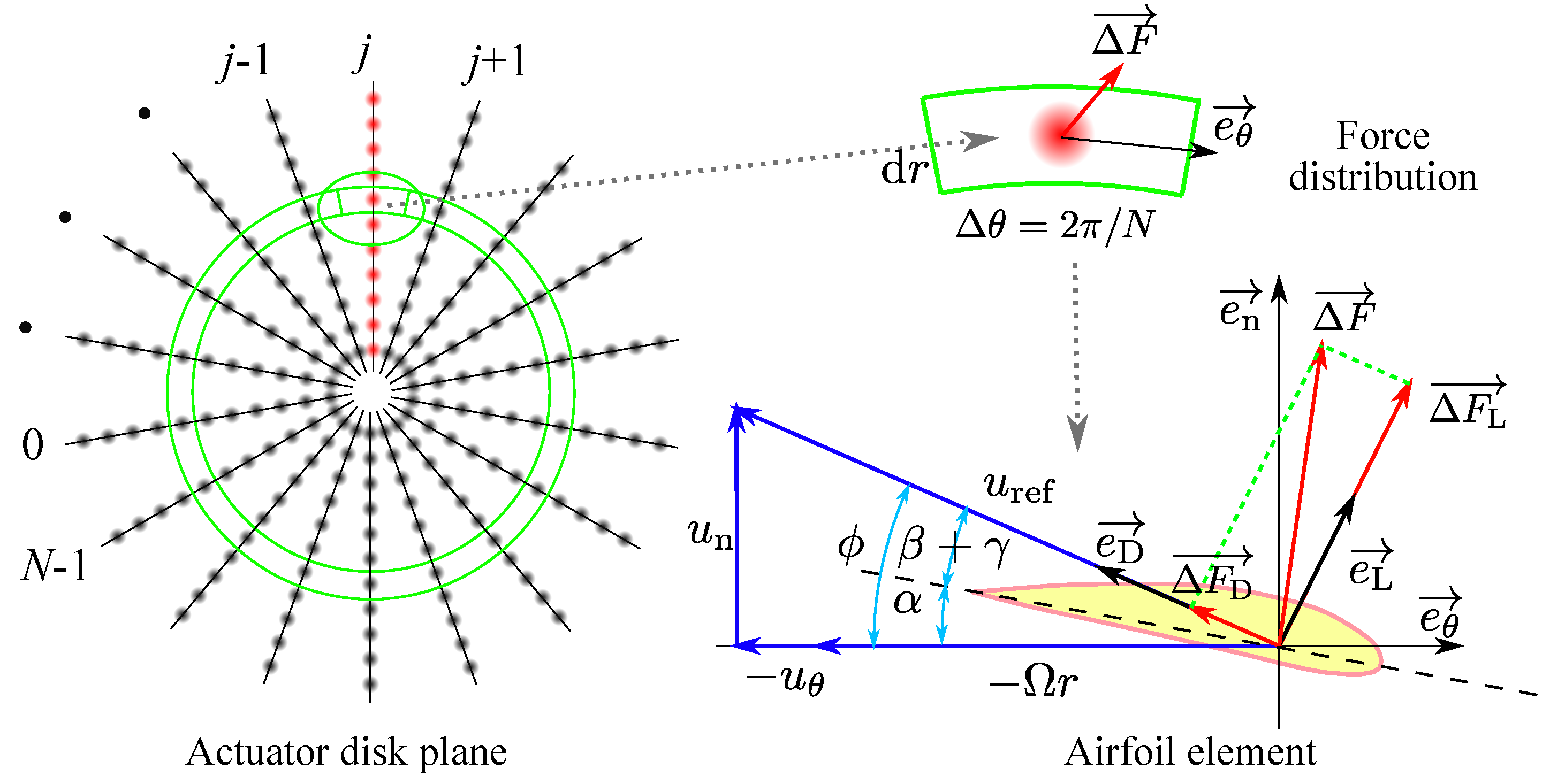
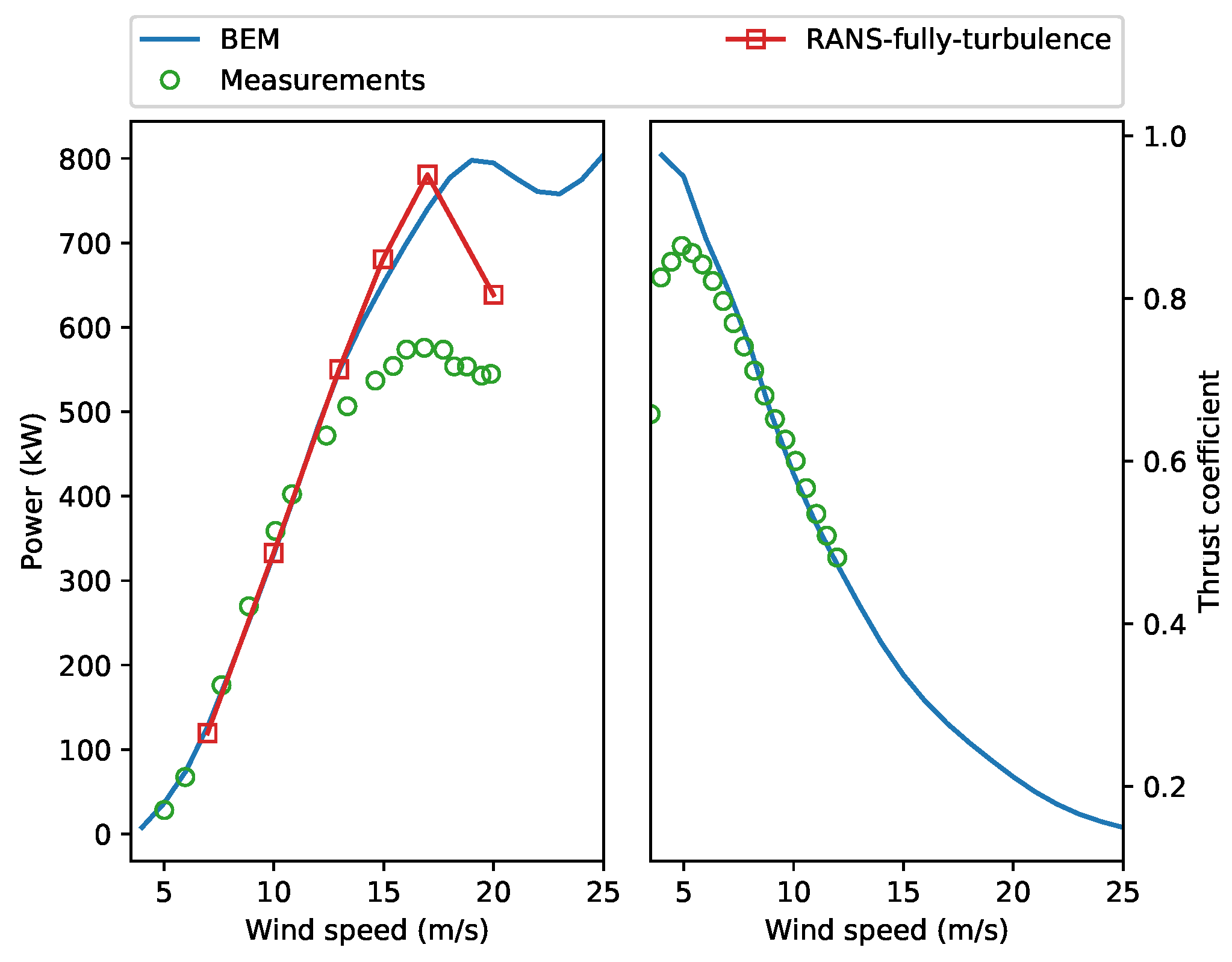
3.1.2. Actuator Disk Model Based on Blade Element Method

In the BEM-based actuator disk model, the rotor plane consists of N actuator lines and each of the actuator lines is split into M element sections (Figure 1). The element section collects the local velocity and the rotor speed $\Omega$ to calculate the element force and applies this force in the neighbor cells of the element section. The reference velocity is firstly assessed from the disk-averaged velocity and is then applied to evaluate the rotor speed.

By transforming the local velocity at the blade element into polar velocity components ($u_r$, $u_{\theta }$, and $u_n$), the force of the blade element is

$$\overrightarrow{\Delta F}=\frac{B\Delta \theta }{4\pi }\rho u_{rel}^{2}c(C_L\overrightarrow{e_L}+C_D\overrightarrow{e_D})\Delta r$$

(18)

where B is the number of the blades, c is the chord length, and $\Delta r$ is the length of the element section. The drag coefficient of the element section, $C_D$, and its lift coefficient, $C_L$, which are functions of the attack angle $\alpha$, are estimated from XFOIL [26] and then corrected by three-dimensional rotational effects of the blades based on Du et al. [27]. According to Figure 1, $\alpha =\varphi -(\beta +\gamma )$, where $\varphi =arctan\left[u_{\mathrm{n}}/(\Omega r+u_{\theta })\right]$ is the flow angle, $\beta$ is the blade installation angle, and $\gamma$ is the pitch angle.

The element force is distributed across neighbor cells. The force added to a cell is calculated by

$$\overrightarrow{\Delta F_{\mathrm{cell}}}=\sum _i^{N·M}\frac{1}{s^3{\pi }^{3/2}}exp\left(-\frac{s_i^2}{s^2}\right)\overrightarrow{\Delta F_i}{F}_{\mathrm{tip}}{F}_{\mathrm{hub}}\Delta V_{\mathrm{cell}}$$

(19)

where $s_i$ the distance of the i-th element to the cell and s is the cut-off length scale that takes a value between 2 and 3 cell sizes [28]. $F_{\mathrm{tip}}$ and $F_{\mathrm{hub}}$ are the Prandtl tip loss and hub loss functions [29]:

$$F_{\mathrm{tip}}=\frac{2}{\pi }arccos\left[exp\left(\frac{B(R-r)}{2rsin\varphi }\right)\right]$$

(20)

$$F_{\mathrm{hub}}=\frac{2}{\pi }arccos\left[exp\left(\frac{B(r-R_{\mathrm{hub}})}{2rsin\varphi }\right)\right]$$

(21)

where R is the rotor radius, $R_{\mathrm{hub}}$ is the hub radius, and r is the radial distance of the element to the rotor center.

3.2. Turbulence Modeling

In this paper, we apply the $k-\epsilon$ turbulence model to close Equations (12)–(14):

$$\frac{\partial }{\partial t}\left(\rho k\right)+\frac{\partial }{\partial x_i}\left(\rho U_{i}k\right)=\frac{\partial }{\partial x_j}\left[\left(\mu +\frac{{\mu }_t}{{\sigma }_k}\right)\frac{\partial k}{\partial x_j}\right]+\mathcal{P}+\mathcal{B}-\rho \epsilon -S_{k,\mathrm{ABL}}$$

(22)

$$\frac{\partial }{\partial t}\left(\rho \epsilon \right)+\frac{\partial }{\partial x_i}\left(\rho U_i\epsilon \right)=\frac{\partial }{\partial x_j}\left[\left(\mu +\frac{{\mu }_t}{{\sigma }_{\epsilon }}\right)\frac{\partial \epsilon }{\partial x_j}\right]+\left(C_{\epsilon 1}\mathcal{P}-\rho C_{\epsilon 2}\epsilon +C_{\epsilon 3}\mathcal{B}\right)\frac{\epsilon }{k}+S_{\epsilon ,\mathrm{wake}}$$

(23)

where k is the turbulence kinetic energy (TKE), $\epsilon$ is the TKE dissipation, $C_{\mu }=0.033$, ${\sigma }_k=1.0,{\sigma }_{\epsilon }=1.3,$ and $C_{\epsilon 2}=1.92$. $\mathcal{P}$ and $\mathcal{B}$ are the TKE source production due to shear and buoyancy, respectively:

$$\mathcal{P}\equiv -\rho \overline{u_i^{\prime }{u}_j^{\prime }}\frac{\partial U_j}{\partial x_i}={\mu }_t\left(\frac{\partial U_i}{\partial x_j}+\frac{\partial U_j}{\partial x_i}\right)\frac{\partial U_j}{\partial x_i}$$

(24)

$$\mathcal{B}\equiv \frac{g_i}{{\Theta }_0}\overline{u_i^{\prime }{\theta }^{\prime }}=-\frac{g_i}{{\Theta }_0}\frac{{\mu }_t}{P{r}_t}\frac{\partial \Theta }{\partial x_i}$$

(25)

where $u_i^{\prime }$ is the fluctuation of the velocity component in $x_i$ direction. $S_{\epsilon ,\mathrm{wake}}$ is a source term of TKE dissipation applied in the neighbor region of the turbine to correct the fast wake recovery of the standard $k-\epsilon$ model [30]:

$$S_{\epsilon ,\mathrm{wake}}=\rho C_{4\epsilon }\frac{{\mathcal{P}}^2}{\rho k}$$

(26)

where $C_{4\epsilon }=0.37$.

In this work, the methods of Alinot and Masson [15], the recently proposed model from M.P. van der Laan et al. [16], and the indirect model that cannot solve the energy equation applied in W.A. El-Askary et al. [14] are investigated, and the models are hereafter referred to as the AM, Laan, and El-Askary models, respectively. In the Laan model and its modified model (the proposed model), the TKE source term $S_{\epsilon ,\mathrm{ABL}}$ and the coefficient $C_{\epsilon 3}$ are functions of atmospheric stability and modeled to keep flow homogeneity under stable conditions. However, $S_{\epsilon ,\mathrm{ABL}}$ is absent in the AM model and the El-Askary model, and $C_{\epsilon 3}$ is set to −2.9 in the AM model [15] and set to 1 in the El-Askary model [14].

In the El-Askary model, the energy Equation (14) is not solved, and the TKE production due to buoyancy $\mathcal{B}$ is modeled as

$$\mathcal{B}=-{\mu }_t{\left(\frac{\partial u}{\partial z}\right)}^2\frac{Ri}{{\varphi }_m}$$

(27)

where

$$Ri=\zeta \frac{0.74+4.7\zeta }{{(1+4.7\zeta )}^2},\zeta >0$$

(28)

The Laan model is derived from homogeneous steady flows over flat terrain where the kinematic viscosity $\mu$ can be ignored, and the $k-\epsilon$ model can be rewritten into normalized form by $\kappa z/u_{*}^3$

$${\varphi }_{t,k}+{\varphi }_m-{\varphi }_{\epsilon }-\frac{{\varphi }_h}{P{r}_t{\varphi }_m}\zeta -{\varphi }_{S_k}=0$$

(29)

$${\varphi }_{t,\epsilon }+\left(C_{\epsilon 1}{\varphi }_m-C_{\epsilon 2}{\varphi }_{\epsilon }-C_{\epsilon 3}\frac{{\varphi }_h}{P{r}_t{\varphi }_m}\zeta \right)\frac{\epsilon }{k}=0$$

(30)

in which ${\varphi }_{t,k}\equiv \frac{\kappa z}{\rho u_{*}^3}\frac{\partial }{\partial z}\left(\frac{{\mu }_t}{{\sigma }_k}\frac{\partial k}{\partial z}\right)$ and ${\varphi }_{t,\epsilon }\equiv \frac{\kappa z}{\rho u_{*}^3}\frac{\partial }{\partial z}\left(\frac{{\mu }_t}{{\sigma }_{\epsilon }}\frac{\partial \epsilon }{\partial z}\right)$ are the normalized turbulent transport of k and $\epsilon$, ${\varphi }_{S_k}\equiv \frac{\kappa z}{u_{*}^3}{S}_{k,\mathrm{ABL}}$, respectively.

Under neutral conditions where $\zeta \to 0$ and ${\varphi }_m,{\varphi }_k,{\varphi }_{\epsilon }\to 1$, Equation (30) reduces to

$$C_{\mu }^{1/2}{\sigma }_{\epsilon }\left(C_{\epsilon 2}-C_{\epsilon 1}\right)={\kappa }^2$$

(31)

which yields $C_{\epsilon 1}=1.24$.

Under stable conditions, we have

$$S_{k,\mathrm{ABL}}=\left\{{\varphi }_m-{\varphi }_{\epsilon }-\frac{{\varphi }_h}{P{r}_t{\varphi }_m}\zeta +\frac{C_{\mu }^{-1/2}{\kappa }^2}{{\sigma }_k}\frac{{\zeta }^2}{{\varphi }_m}\left[{\varphi }_k^{{}^{″}}-\frac{{\varphi }_k^{{}^{\prime }}{\varphi }_m^{{}^{\prime }}}{{\varphi }_m}+\frac{{\varphi }_k^{{}^{\prime }}}{\zeta }\right]\right\}\frac{u_{*}^3}{\kappa z}$$

(32)

$$\frac{{\varphi }_h}{P{r}_t{\varphi }_m}{C}_{\epsilon 3}=\frac{C_{\epsilon 1}{\varphi }_m-C_{\epsilon 2}{\varphi }_{\epsilon }}{\zeta }+\frac{C_{\mu }^{-1/2}{\kappa }^2}{{\sigma }_{\epsilon }}\frac{{\varphi }_k}{{\varphi }_m}\left[\frac{\zeta {\varphi }_{\epsilon }^{{}^{″}}}{{\varphi }_{\epsilon }}-\frac{\zeta {\varphi }_{\epsilon }^{{}^{\prime }}{\varphi }_m^{{}^{\prime }}}{{\varphi }_{\epsilon }{\varphi }_m}-\frac{{\varphi }_{\epsilon }^{{}^{\prime }}}{{\varphi }_{\epsilon }}+\frac{{\varphi }_m^{{}^{\prime }}}{{\varphi }_m}+\frac{1}{\zeta }\right]$$

(33)

where ${\varphi }^{\prime }=\partial \varphi /\partial \zeta$ and ${\varphi }^{″}={\partial }^2\varphi /\partial {\zeta }^2$ for $\varphi \in \{{\varphi }_k,{\varphi }_m,{\varphi }_{\epsilon }\}$. Equations (32) and (33) allow turbulence closure that is consistent with either the classical similarity functions in MOST (the Laan model) or any other similarity functions based on field measurements (the proposed model in this paper). One can prove that the above equations equal to those proposed by van der Laan et al. [16] if the classical similarity functions are applied. Note that the turbulent Prandtl number is set to 1 in the origin AM model and the Laan model, and the energy Equation (14) is also not solved in the Laan model. This work, however, applies $P{r}_t\equiv {\varphi }_h/{\varphi }_m$ according to the definition of the turbulent Prandtl number [31] and solves the energy Equation (14) in the Laan model. There are negligible differences in wake modeling when considering these differences in implementations of the models. Details of the turbulence models investigated in this paper are summarized in

Table 1. Summary of turbulence models investigated for stable conditions, where “−” represents that the corresponding term is absence in the model, “√” represents that the energy equation is solved, and “classical” denotes standards for the classical similarity functions.

Turbulence Model	Energy Equation (14)	$\mathcal{B}$	${\mathit{S}}_{\mathit{k},\mathbf{ABL}}$	${\mathit{C}}_{3\mathit{\epsilon }}$	Similarity Functions
AM	√	Equation (25)	−	−2.9	classical
El-Askary	−	Equation (27)	−	1	classical
Laan	√	Equation (25)	Equation (32)	Equation (33)	classical
Proposed	√	Equation (25)	Equation (32)	Equation (33)	${\varphi }_{m,\exp }$, ${\varphi }_{h,\exp }$, ${\varphi }_{\epsilon ,\mathrm{cls}}$

.

4. Breakdown and Modifications of MOST under Stable Conditions

This section shows the breakdown of MOST in predicting the velocity gradient under stable conditions and proposes a set of new similarity functions to eliminate this side effect. All these works are based on a field experiment over complex terrain in a wind farm. The influence of complex terrain on estimating similarity functions is investigated and assessed for predicting wind profiles.

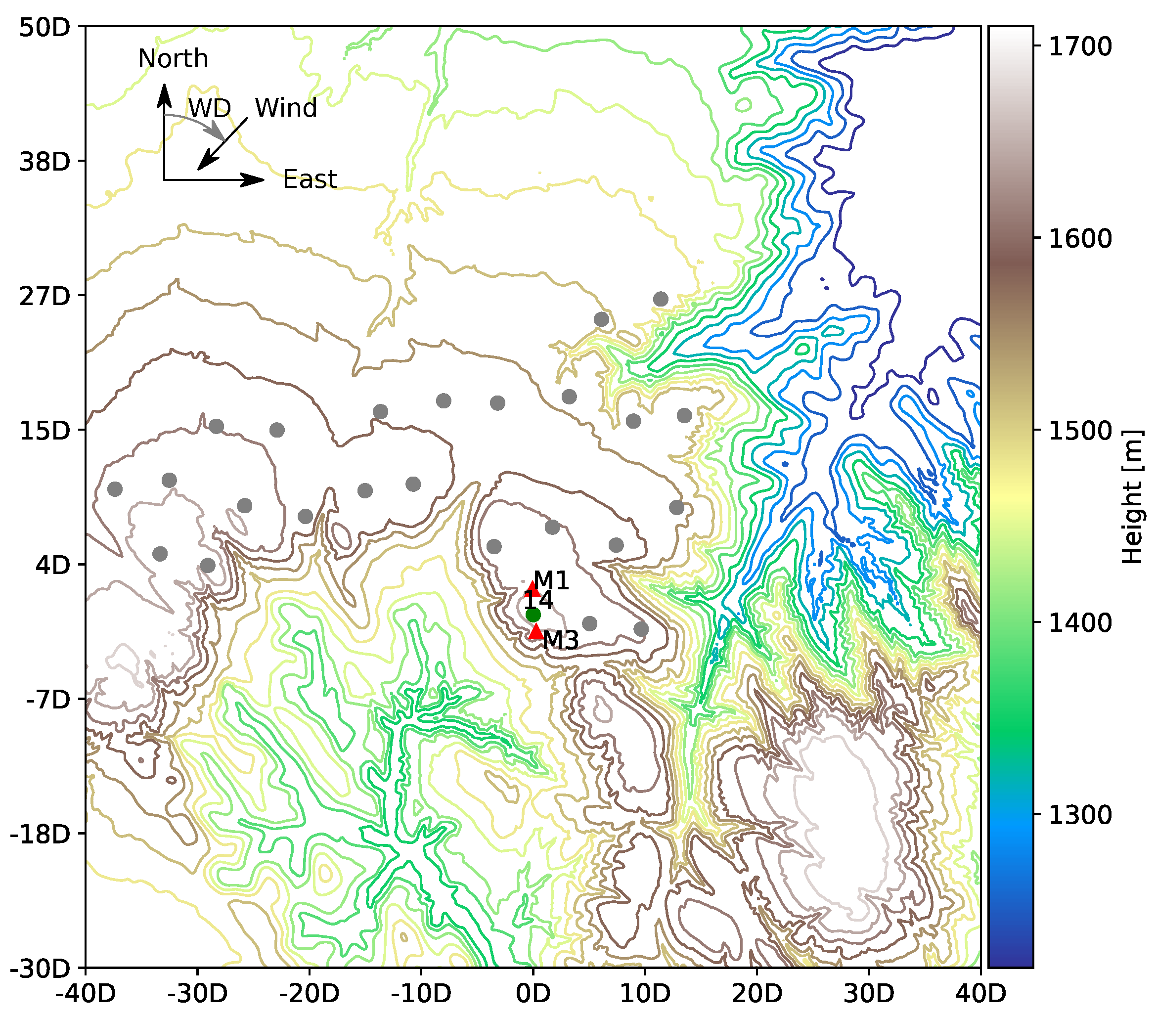
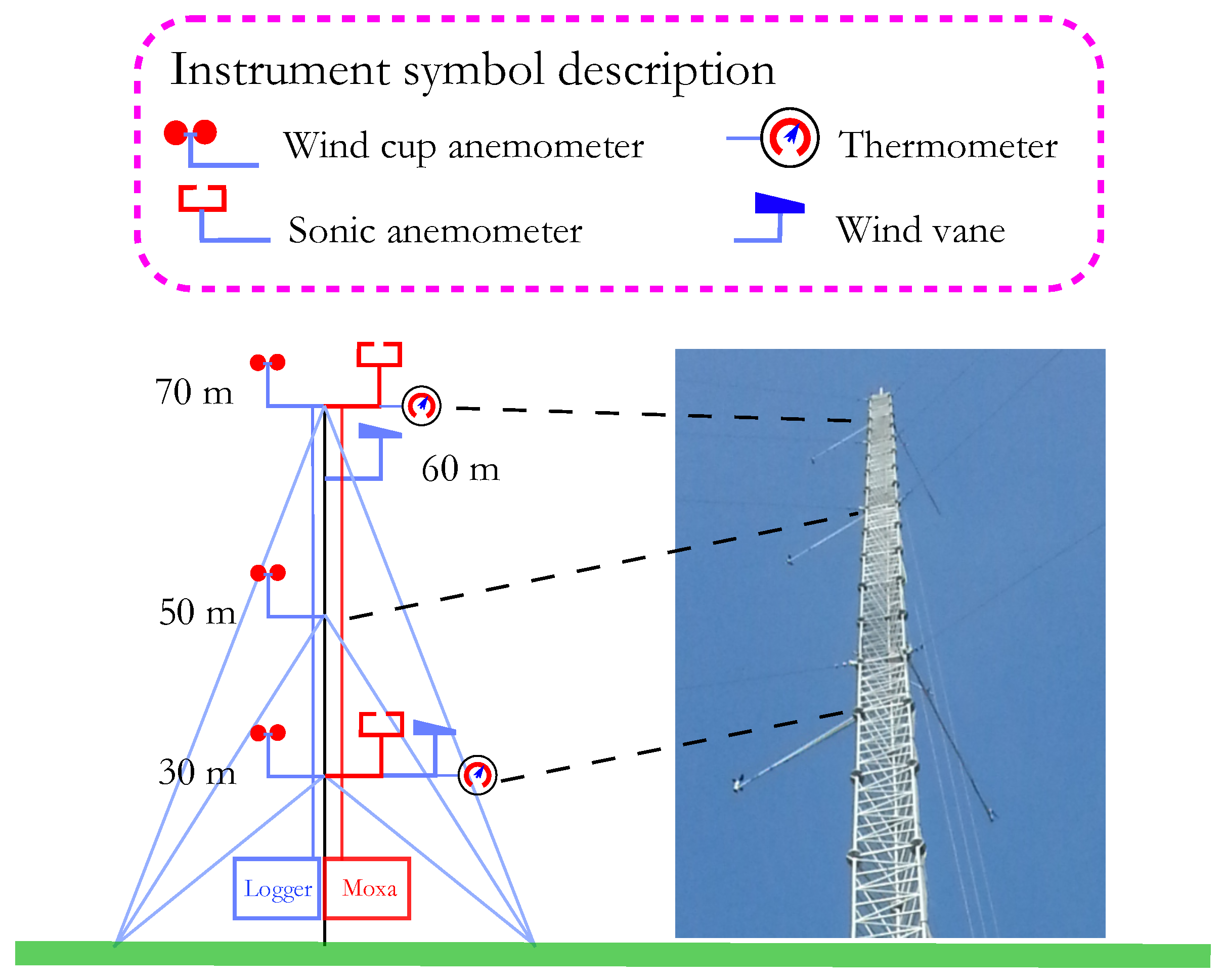
4.1. Experimental Data

The field experiment used to investigate the similarity functions was carried out in the Jingbian wind farm in northwest of China [2]. In the experimental campaign, two masts, numbered M1 and M3, are installed near a wind turbine (No. 14) to capture the wake profiles (Figure 2). As the inflow from north is dominated by a small and constant terrain slope while the inflow from east and south are dominated by a significant terrain complexity, we applied measurements from the mast M1 to estimate similarity functions. On the mast M1, three Thies First Class Advanced cup anemometers were installed at 30 m, 50 m, and 70 m above the ground level (AGL) (Figure 3). Wind direction (WD) was measured at 30 m and 60 m AGL, and air temperature was measured at 30 m and 70 m AGL, respectively. Two Metek 3D sonic anemometers were installed on M1 to provide three-dimensional velocity components and sonic temperature at 30 m and 70 m AGL in a frequency of 35 Hz. A NRG logger was used to record the 10-min statistical values from the cup anemometers, wind vanes, and thermometers. The measured data are resampled to 10 min in ~190 days.

All the anemometers are calibrated in wind tunnels to compensate flow distortion effects. The classification of cup anemometers after calibrations is class A 1.5–1.8 [32], suggesting an uncertainty within ±2.3% for the wind speed above 3 m/s according to IEC 61400-12-1 [33]. In [34], a total uncertainty of 3.6% for the wind speed can be assessed as the root sum of squared uncertainties, due to the sensor accuracy (2.3%), the sensor calibration (2%) [35], and the mounting of anemometers on the mast (2%) [36]. For the sonic anemometers, the 10-min averaged wind speeds recorded by cup anemometers and sonic anemometers at the same heights agree well with slopes close to 1 and correlation coefficients above 0.993 (Figure 4).

Note that the field experiment was carried out in a wind farm in complex terrain. Wind turbine wakes and complex terrain could influence estimating similarity functions. As the wake structure is nonlinear and aligned with wind direction, Han et al. selected the dataset in wind direction sectors with high wind speed correlation to eliminate wake effects for the same measurement campaign [2]. Based on their work, we choose three wind direction intervals, (1) the north section: WD $=0^{\circ }\pm {10}^{\circ }$; (2) the east section: WD $={60}^{\circ }\pm 5^{\circ }$; and (3) the west section: WD $={250}^{\circ }\pm {40}^{\circ }$, to study similarity functions where WD stands for the wind direction, and the intervals are kept narrow, if possible, to ensure data quality with more than 400 points of data. According to Figure 2, the inflow wind in the east and west sections are dominated by complex terrain while the inflow from the north section is dominated by a small slope terrain (slope $\approx {2.4}^{\circ }$). Therefore, the three wind direction intervals are also applied to study the influence of terrain on the estimation of similarity functions.

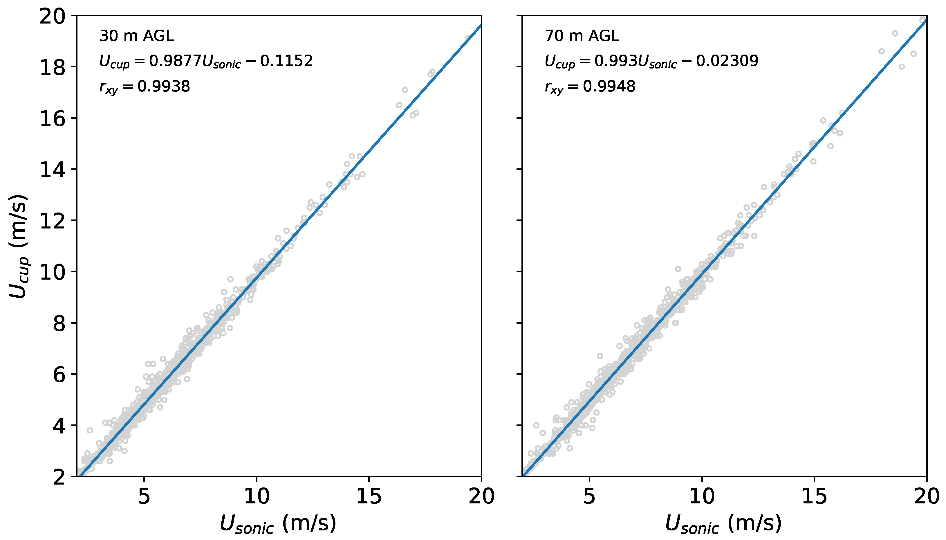
4.2. Data Processing

The heat flux $\overline{w^{\prime }{\theta }^{\prime }}$, the Obukhov length L, and the friction speed $u_{*}$ are evaluated based on measurements of the sonic anemometers [2]. In reference to Högström [37], we enforce the criteria (1) $u_{*}\ge 0.1$ m/s for the ${\varphi }_m-$analysis and (2) $|H_S|\ge 10$ W·m${}^{-2}$ and $u_{*}\ge 0.1$ m/s for the ${\varphi }_h-$analysis, where $H_S=\rho c_p\overline{w^{\prime }{\theta }^{\prime }}$ is the flux of sensible heat and $c_p=1004$ J·(K·kg)${}^{-1}$ is the constant pressure specific heat of air. The local gradients could be derived using the profile-fitting methods of Nieuwstadt [38] or Högström [37] with more than four levels available to fit profiles of velocity and temperature. However, wind speeds and temperatures are only measured at three and two levels, respectively. To avoid overfitting profiles, the velocity and temperature gradients are approximated at the geometric mean height of levels $z_1=30$ m and $z_2=70$ m by the finite difference form [39,40]

$$\frac{\partial \Phi }{\partial z}\approx \frac{\Phi \left(z_2\right)-\Phi \left(z_1\right)}{\sqrt{z_1{z}_2}ln(z_2/z_1)}$$

(34)

where $\Phi \in \{U,\Theta \}$. It is easy to prove that this expression is rigorous for logarithmic profiles and has an error within ±3% for log-linear profiles predicted by MOST.

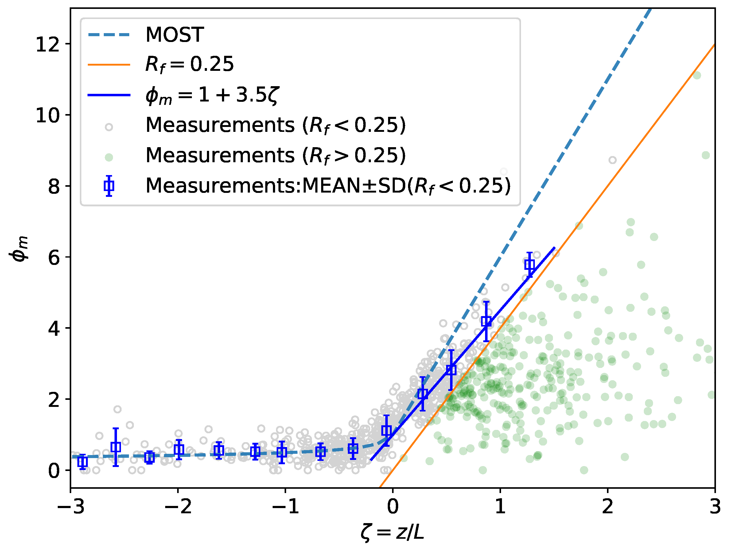
4.3. Limitations and Breakdown of MOST

In this section, we show that the classical ${\varphi }_m$ consistent with MOST is not valid for $R_f>0.25$, based on the measured data of the sonic anemometer at 30 m a.g.l for WD = $0^{\circ }\pm {10}^{\circ }$. The flux Richardson number $R_f$ is defined as

$$R_f\equiv -\frac{\frac{g}{\Theta }\overline{w^{\prime }{\theta }^{\prime }}}{u_{*}^2\frac{\partial U}{\partial z}}$$

(35)

Combining the definitions of L and $R_f$, we have

$${\varphi }_m\left(\zeta \right)=\zeta /R_f$$

(36)

which indicates that $R_f=0.25$ is a straight line in the plane $\zeta -{\varphi }_m$. Figure 5 shows that the line $R_f=0.25$ split the measured data into two groups: for $R_f<0.25$, the measured data have good agreements with the data predicted by MOST under unstable conditions and show a linear prediction of ${\varphi }_m$, with ${\beta }_m=0.35$ under stable conditions; for $R_f>0.25$, the measured data are significantly lower than those predicted by MOST. For wind energy applications, measured data are usually mixed, and engineers commonly focus on wind turbine wakes under stable conditions without considering the limitation of $R_f$. In this situation, MOST could overestimate the velocity gradient and potentially influence wake modeling of a wind turbine.

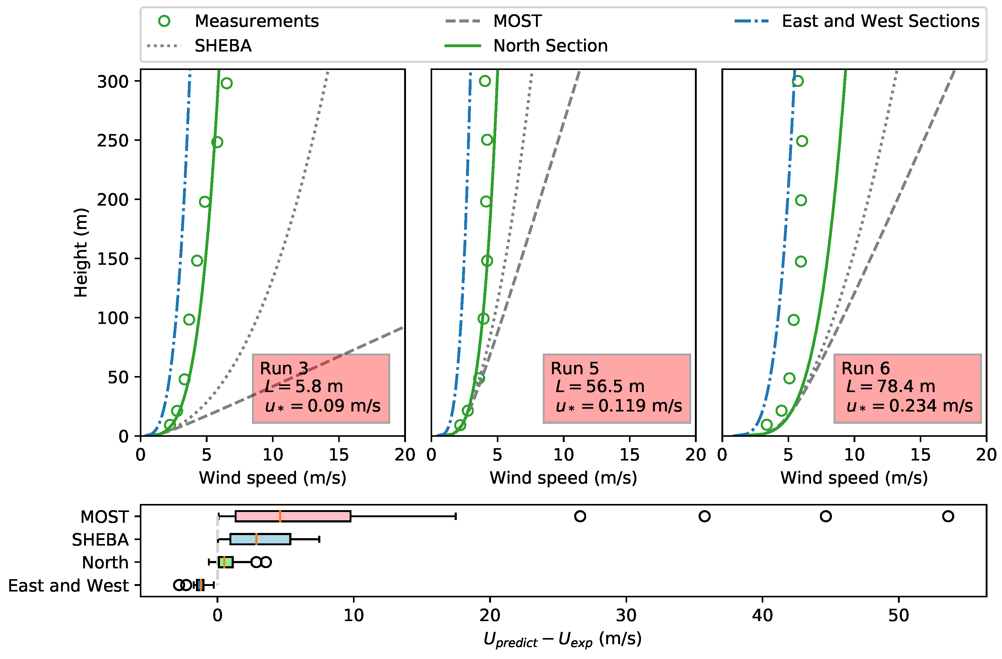
4.4. Assessment of Similarity Functions for Predicting Wind Profiles

Plots of the dimensionless velocity gradients versus the stability parameter in three wind direction intervals are presented in Figure 6. For the three wind direction intervals, the upslope inflows towards the mast are accelerated more at low levels than at high levels [41], and the dimensionless velocity gradient is decreased consequently. For the east and west sections in complex terrain, the fitted ${\varphi }_m$ based on field measurements is 30% lower than that of the north section, with a small slope terrain for $0<\zeta <0.1$. Similarly, a decrease of 30% in ${\varphi }_m$ ($=0.7+1.5\zeta$) was also observed in a stable boundary layer over the complex terrain of the Loess Plateau, China [42]. The fitted ${\varphi }_m$ are also compared with the classical similarity function ${\varphi }_{m,\mathrm{cls}}=1+{\beta }_m\zeta$ and the SHEBA profile function ${\varphi }_{m,\mathrm{SHEBA}}=1+6.5\zeta {(1+\zeta )}^{1/3}/(1.3+\zeta )$ [43]. As shown in Figure 6, all the fitted ${\varphi }_m$ and the SHEBA profile function can limit the velocity gradient under strongly stable conditions: ${\varphi }_m\propto {\zeta }^{1/4}$ (fitted) and ${\varphi }_m\propto {\zeta }^{1/3}$ (SHEBA) for $\zeta \to \infty$. For the north section where the inflows are dominated by a small slope, ${\varphi }_{m,\mathrm{cls}}$ and ${\varphi }_{m,\mathrm{SHEBA}}$ agree well with measurements for $\zeta <0.1$ and overestimate the velocity gradient for $\zeta >0.1$. Affected by complex terrain, the fitted ${\varphi }_m$ estimated for the east and west sections are much lower than ${\varphi }_{m,\mathrm{cls}}$ and ${\varphi }_{m,\mathrm{SHEBA}}$.

The fitted similarity functions are evaluated for predicting wind profiles based on the Boulder Atmospheric Observatory (BAO) dataset [44]. Among the seven runs presented in Sorbjan et al. [44], only runs 3, 5, and 7 are studied, due to the criteria $|H_S|\ge 10$ W·m${}^{-2}$. The wind profiles predicted by varying similarity functions are presented in Figure 7 and estimated in numerical integration by

$$U\left(z\right)={\int }_{z_0}^z\frac{u_{*}}{\kappa z}{\varphi }_m\left(\frac{z}{L}\right)\mathrm{d}z$$

(37)

where the aerodynamic rounghess $z_0$ is ~0.01 m for the BAO dataset [44]. According to Figure 7, the fitted ${\varphi }_m$ of the north section performs better in predicting wind profiles for runs 3, 5, and 6, whereas ${\varphi }_{m,\mathrm{cls}}$ and ${\varphi }_{m,\mathrm{SHEBA}}$ overestimate the velocity gradient significantly. The wind speed is overestimated on average by 4.6 m/s, 3 m/s, and 0.5 m/s for ${\varphi }_{m,\mathrm{cls}}$, ${\varphi }_{m,\mathrm{SHEBA}}$ and the fitted ${\varphi }_m$ of the north section, respectively. Influenced by complex terrain, the fitted ${\varphi }_m$ of the east and west sections underpredicts the velocity of 1.2 m/s averagely. As ${\varphi }_m\left(0\right)<1$ of the east and west sections disagrees with the logarithmic law of wind profiles in flat terrain under neutral conditions [45,46], we apply the similarity functions estimated from the dataset of the north section in the wake simulations.

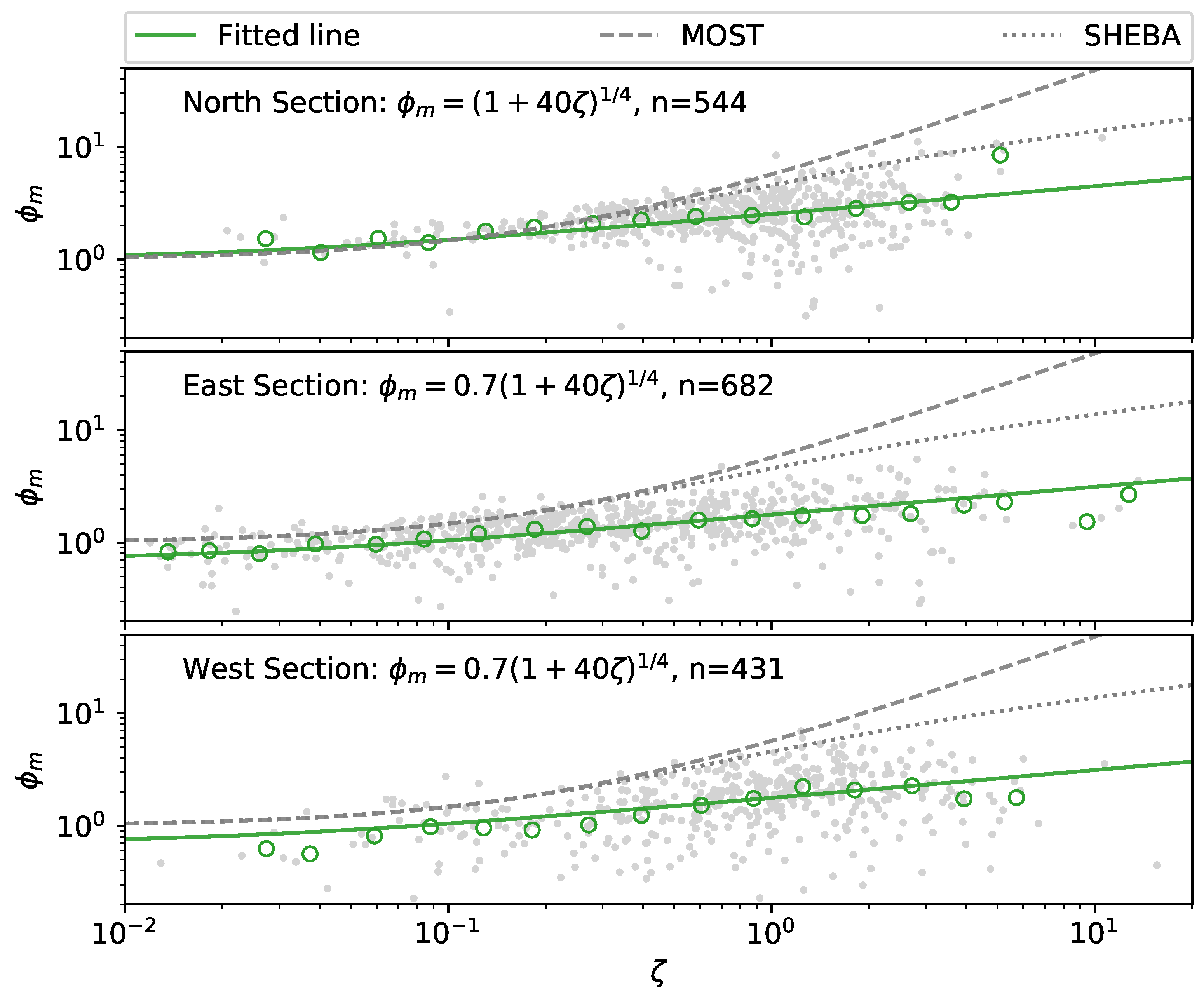
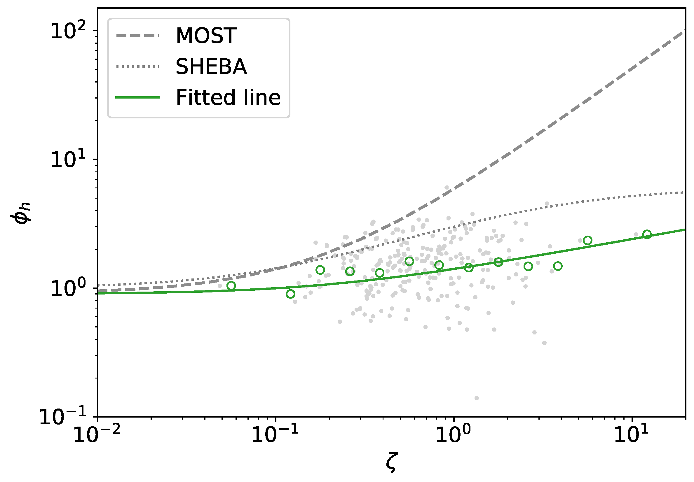
4.5. The Proposed Similarity Functions

In the full range of $R_f$, the corresponding proposed similarity functions based on the dataset of the north section under stable conditions are as follows,

$${\varphi }_{m,\exp }\left(\zeta \right)={(1+40\zeta )}^{1/4}$$

(38)

$${\varphi }_{h,\exp }\left(\zeta \right)=\chi {\left(1+5\zeta \right)}^{1/4}$$

(39)

where $\chi =0.9$. The dimensionless temperature gradient is observed significantly lower than the classical value for $\zeta >0.1$ (Figure 8). Grachev et al. [31,43] also observed a similar phenomenon and then proposed a corresponding function: ${\varphi }_{h,\mathrm{SHEBA}}=1+5\zeta (1+\zeta )/(1+3\zeta +{\zeta }^2)$.

5. Simulation Details

5.1. Test Cases

In this work, under stable conditions, we investigate the wakes of a 500 kW NTK500/41 wind turbine at the Risø Campus test site of DTU in Denmark [1] and three 180 kW Danwin turbines on the island of Gotland in the Baltic Sea [6]. The two test cases cover wake measured data 1D to 9D downstream of the turbines where D is the rotor diameter. Details of test cases are listed in

Table 2. Details of measurements in the two test cases.

Wind Turbine	D (m)	H (m)	Measurements	Wake Range
NTK500/41	41	36	LiDAR scanning	1D to 5D
Danwin	23	35	Mast measurements	4.2D, 6.1D, and 9.6D

.

The first case is based on LiDAR measurements of the wakes of a NTK500/41 turbine. In this campaign, a pulsed LiDAR, which was mounted on a platform at the rear of the nacelle, pointed its laser downstream the turbine up to 5D downstream the turbine. A constant downhill slope of about 0.3% was observed downstream the turbine. Inlet meteorological properties, such as wind speed, wind direction, air temperature, and atmospheric pressure, were measured from a 57-m-tall meteorological mast located upstream the turbine. The NTK500/41 turbine is a stall-regulated 500 kW wind turbine equipped with LM 19.1 m blades and its rotor speed is fixed at 27.1 rpm. Its blades consist of two kinds of airfoils: FFA-W3-XX1 (from 16 to 50% span) and NACA 63-XXX (from 60 to 100% span) [47]. Chord length and twist angle over the blades were presented in Johansen et al. [48]. The power curve and the thrust coefficient curve based on BEM calculations are shown in Figure 9. The power curve from BEM calculations is shown to have good agreement with the RANS computations in the full turbulence model [48] below 15 m/s and measurements [48] below 10 m/s (Figure 9). The measured thrust coefficient from strain gauges measurements [49] is also shown to have good agreements with the BEM computations above 6 m/s. In this case, we set $z_0=0.095$ m, $L=29$ m, and the hub-height reference wind speed $U_{\mathrm{hub}}=6.76$ m/s, as presented in Machefaux et al. [1], and apply $C_T=0.83$ based on the BEM computations.

The second case is based on wake measurements of three Danwin wind turbines using two 54 m meteorological masts, M1 and M2. In the campaign, the masts were equipped with wind sensors at 8 levels from 10 m to 53.3 m. Inlet conditions including temperature profiles were measured on mast M1, whereas wake profiles of the three turbines were measured on mast M2. The distances from the three turbines to mast M2 are 4.2D, 6.1D, and 9.6D, respectively. In this case, we set the roughness length, the Obukhov length, the reference wind speed and the thrust coefficient to be 0.0005 m, 35 m, 8 m/s and 0.82, respectively [6,50]. The detail information of test cases is shown in

Table 3. Test cases and corresponding parameters under stable conditions.

Model	Case 1		Case 2
	${\mathit{u}}_{*}$ (m/s)	TI	${\mathit{u}}_{*}$ (m/s)	TI
AM, Laan, El-Askary	0.223	6.0%	0.198	4.5%
Proposed	0.297	10.2%	0.228	6.5%

where TI $=\sqrt{\frac{2}{3}{k}_{\mathrm{hub}}}/U_{\mathrm{hub}}$ is the ambient turbulence intensity at hub height and $k_{\mathrm{hub}}$ is the corresponding hub-height turbulence kinetic intensity [16]. The measured ambient turbulence intensity in the first case is ~10%.

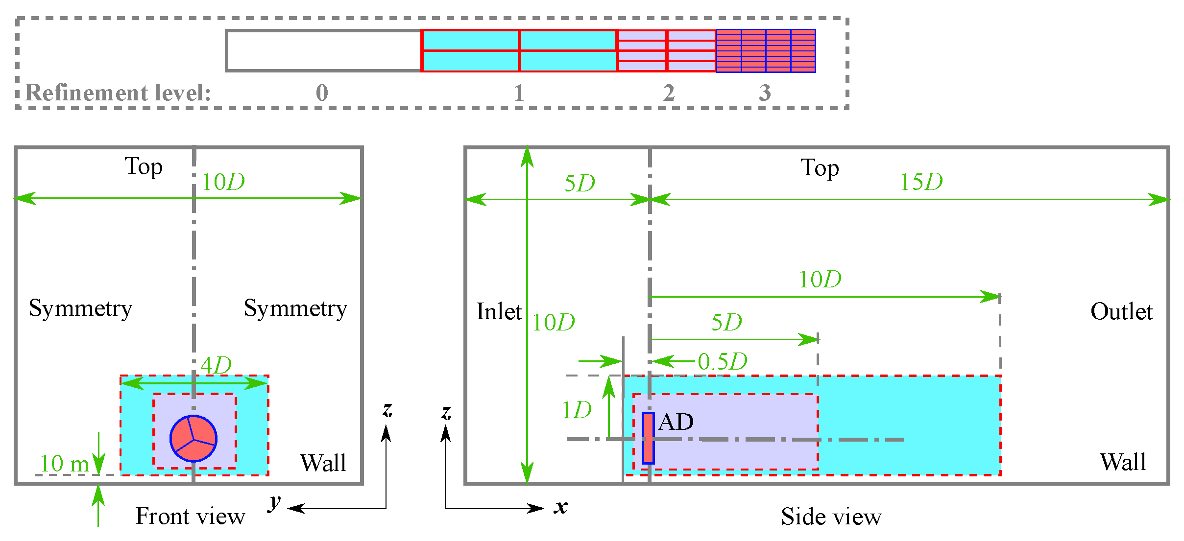
5.2. Computational Domain and Meshing

The computational domain has a length of $20D$, a width of $10D$, and a height of $10D$ (Figure 10). The background mesh, whose refinement level is 0, consists of $100\times 60\times 60$ in length, width, and height. The vertical grids are clustered near the ground and the first cell height above the ground is set to 7.38 $z_0$ to produce appropriate kinetic energy [51]. The mesh around the wind turbine and in the wake region is refined as shown in Figure 10. The mesh is refined around the disk region to ensure about 80 cells through the rotor diameter [52]. The complete mesh is composed of ~1.6 million cells.

5.3. Boundary Conditions

The boundary conditions consistent with similarity functions are applied to modeling the atmospheric boundary stratification. Wind profile at inlet is estimated by Equation (37). The inlet profiles of potential temperature, TKE, and its dissipation are given by

$$\Theta \left(z\right)={\Theta }_0+{\int }_{z_0}^z\frac{{\theta }_{*}}{\kappa z}{\varphi }_h\left(\frac{z}{L}\right)\mathrm{d}z$$

(40)

$$\epsilon =\frac{u_{*}^3}{\kappa z}{\varphi }_{\epsilon }\left(\frac{z}{L}\right)$$

(41)

$$k=\frac{u_{*}^2}{\sqrt{C_{\mu }}}{\varphi }_k\left(\frac{z}{L}\right)$$

(42)

The vertical profiles of potential temperature are estimated in numerical integration. At the outlet, zero gradients of $U,\Theta ,\epsilon ,k$ are applied. For the top boundary, the upstream flow properties are maintained constant. The left and right sides of the computational domain are set to be symmetry.

The near-wall treatment of Temel et al. [53] is implemented in the near ground region to calculate turbulent dissipation rate and the TKE production $G_{k,p}$ due to shear (${\mathcal{P}}_p$) and buoyancy (${\mathcal{B}}_p$):

$${\epsilon }_p=\frac{u_{*k}^3}{\kappa z_p}{\varphi }_{\epsilon ,p}$$

(43)

$$G_{k,p}\equiv {\mathcal{P}}_p+{\mathcal{B}}_p=\frac{{\tau }_w^2}{\rho \kappa u_{*k}(z_p+z_0)}-\frac{{\theta }_{*}\left|g\right|}{{\Theta }_0(z_p+z_0)}$$

(44)

where the subscript p denotes the first cell center above the ground, the equivalent friction wind speed is $u_{*k}=C_{\mu }^{0.25}{\varphi }_{k,p}^{-0.5}{k}_p^{0.5}$, and the wall shear stress is ${\tau }_w={\mu }_{t,p}(\mathrm{d}U/\mathrm{d}z)$. The eddy viscosity ${\mu }_{t,p}$ and the turbulent heat conductivity are imposed at the first cell center above the ground as [54]

$${\mu }_{t,p}=\frac{u_{*k}{z}_p}{{\int }_{z_0}^{z_p}\frac{1}{\kappa z}{\varphi }_m\left(\frac{z}{L}\right)\mathrm{d}z}-\mu$$

(45)

$${\alpha }_{t,p}={\mu }_{t,p}{\varphi }_{m,p}/{\varphi }_{h,p}-\mu /Pr$$

(46)

where the laminar viscosity $\mu$ is not ignored to keep consistent with Equations (13) and (14).

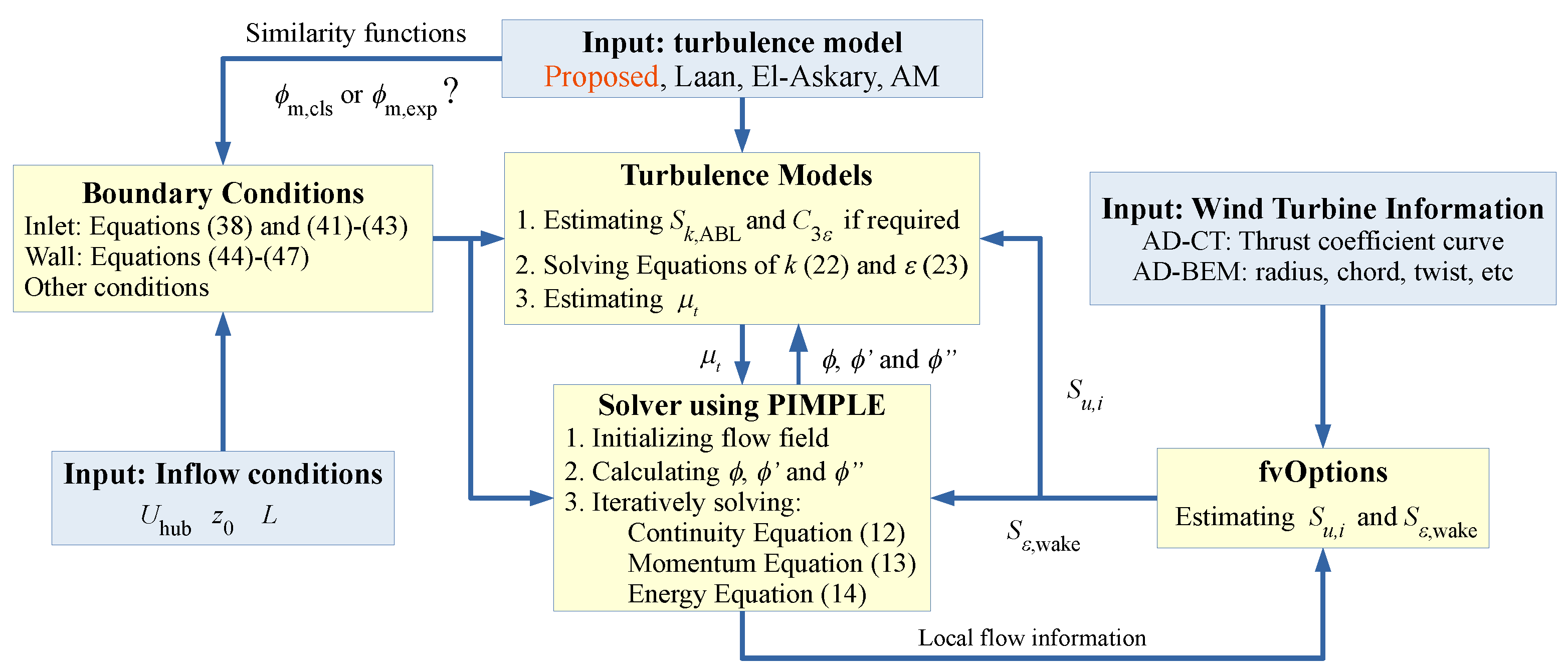
5.4. Implementations of Wake Models

In this paper, wake models are implemented in a CFD framework Open-Source Field Operation And Manipulation (OpenFOAM) [55] for developing customized numerical solvers and pre-/postprocessing utilities for fluid flow problems using the finite-volume method. It allows developing user-defined boundary conditions, turbulence models, and solvers, or adding source terms in a convenient way by extending or modifying existing models. As shown in Figure 11, we implement all the test turbulence models (the proposed, Laan, El-Askary, and AM) and develop a large time-step transient solver using the PIMPLE (merged PISO-SIMPLE) algorithm to simulate wakes of wind turbines under stable conditions. At the beginning of simulations; this solver first initializes the flow field based on boundary conditions. During this period, similarity functions and their derivatives are also evaluated and then used in turbulence models to estimate $S_{k,\mathrm{ABL}}$ and $C_{\epsilon 3}$ if required. This solver then solves the continuity, momentum and energy equations based on the eddy viscosity $\mu$ provided by the turbulence models before in iterations the finish of the simulation. During the iteration, source terms $S_u$ and $S_{\epsilon ,\mathrm{wake}}$ are modeled based on local flow information via user-specified finite volume options (fvOptions). In simulations, we apply a second-order backward difference scheme for temporal discretization and a second-order central difference scheme for spatial discretization of other derivative terms.

6. Results of Wake Simulations

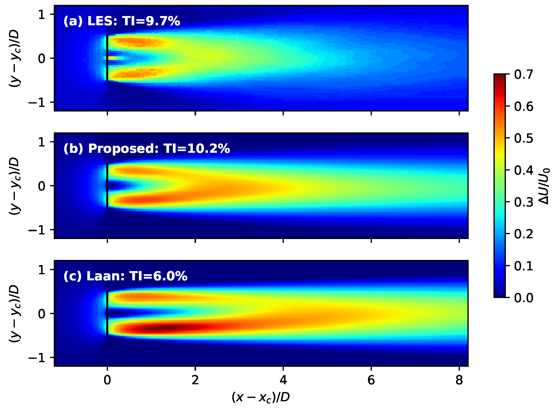
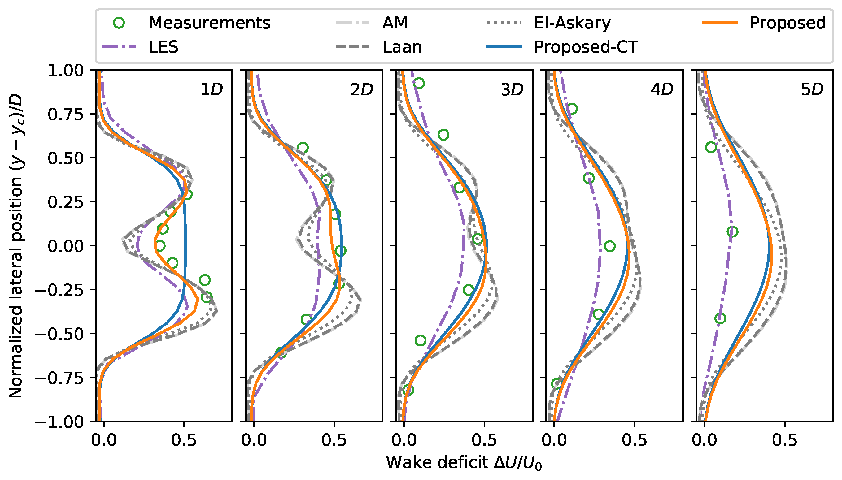
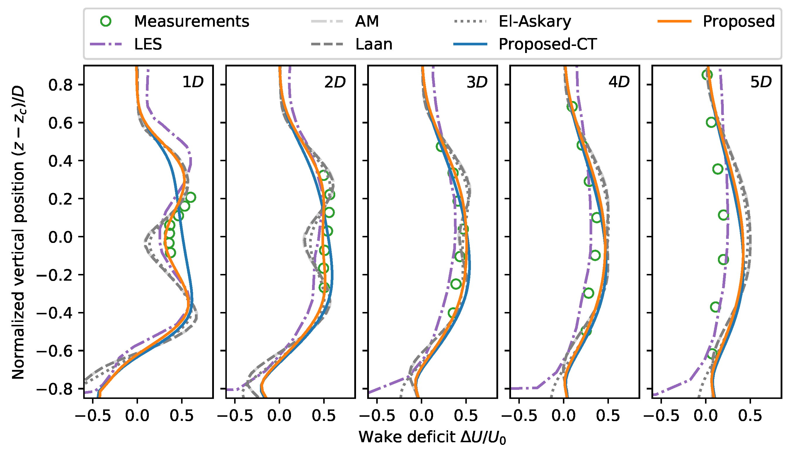
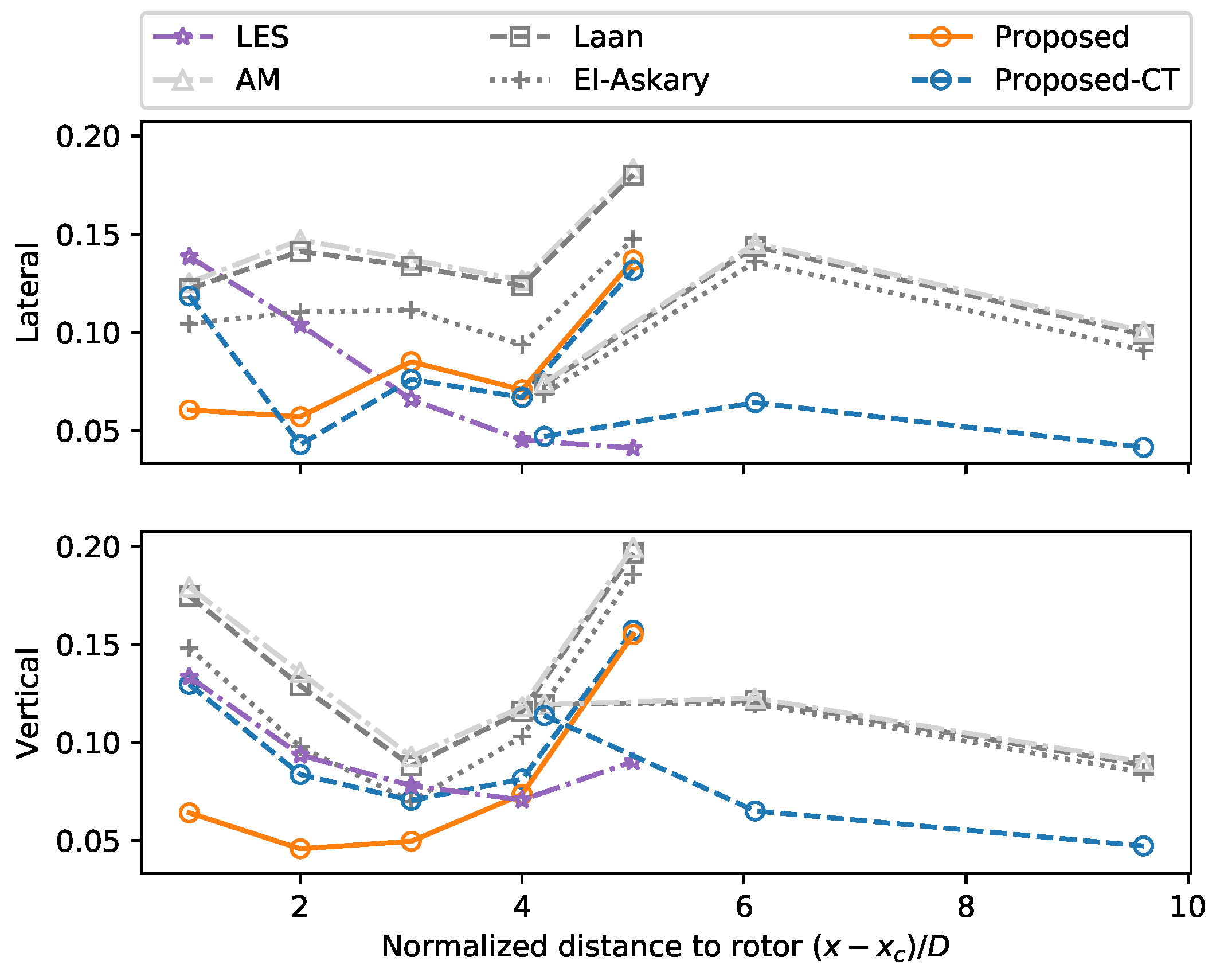
6.1. Case 1: Wakes of a NTK500/41 Wind Turbine

In Machefaux et al. [1], the wakes of a NTK500/41 wind turbine was studied experimentally and numerically using two LES methods: a classical method based on the ELLIPSYS3D flow solver [56] and an extended approach that explicitly introduces thermal and Coriolis effects as external force terms into the solver. As the wind profile predicted by MOST was observed to be much more severely sheared as compared with measurement, the classical approach applied a power law for the inlet velocity profile. The extended LES approach additionally carried out a transient precursor computation to simulate the time-varying vertical structure of the whole ABL, and it used the results of the precursor simulations to impose the mean potential temperature and velocity profiles at the inlet for wake modeling. The precursor simulations are shown to have effects on limiting the overestimated velocity gradient predicted by MOST [1]. Numerical simulations have shown that there are no major differences in wake deficit predictions between the classical approach and the extended model for stable and unstable cases. Therefore, we only compare the wake deficit predicted by the extended approach with the test models in RANS in this work.

Figure 12 shows contours of wake deficits, $\Delta U/U_0$, predicted by different models at hub height under stable conditions, where $\Delta U$ is the velocity deficit in the wake and $U_0$ is the inlet velocity. Simulations using the LES technology show a faster recovery wake than that in the proposed model, whereas the Laan model predicts a significant slower recovery wake with a larger deficit. One possible explanation for the stronger wake effects predicted by the Laan model is that they are due to the lower turbulence intensity predicted by the classical similarity functions. For a given reference wind speed $U_{\mathrm{hub}}$ and a fixed roughness length $z_0$, a higher velocity gradient in the Laan model results in a smaller friction speed $u_{*}$ and a lower turbulence intensity $I_{\mathrm{hub}}$ than the proposed model, and thus it weakens the wake recovery. The ambient turbulence intensities for the LES approach of 9.7% and the proposed model of 10.2% are close to the measured value of 10% while the value for the Laan model is reduced by 40% as compared to the measured data.

As compared with measurements, the proposed model shows better performance than other approaches based on MOST combined with RANS for the longitudinal distance of 1–5D and the LES approach for the longitudinal distance below 3D (Figure 13 and Figure 14). The AM, El-Askary, and Laan models overestimate the wake deficits in both vertical and lateral directions for longitudinal distances above 2D. All the test models in RANS fail to predict wake deficits at 4–5D downstream of the rotor. This disagreement is probably due to a combination of terrain effects and experimental uncertainties using LiDAR. According to the Space Shuttle Topography Mission (STRM)-based terrain data, the test site terrain has a downhill slope characterized by a height difference of 5.5 m from the rotor location to the most downstream cross section. As the wake has been observed to follow terrain under stable conditions [1,8], the wind speed for the longitudinal distance above 5D at the hub height is actually the value of 5.5 m above the wake center, which results in the overestimation of wake by various turbulence models in RANS.

For the vertical profiles of wake deficits, Figure 14 shows that the proposed model overestimates wake deficits below the hub height at $5D$. A double-bell near-wake shape, due to a lower energy extraction around the blade root [1], is clearly observed under stable conditions at 1D and is captured by the actuator models based on BEM calculations. There are no major differences between the vertical wake profiles predicted by the proposed models based on either the thrust coefficient (Proposed-CT) or BEM calculations (Proposed) above $2D$. As the LES model applies slip wall conditions at the bottom of the computational domain and does not consider the roughness effect of the ground, large negative wake deficits are observed near the ground [1].

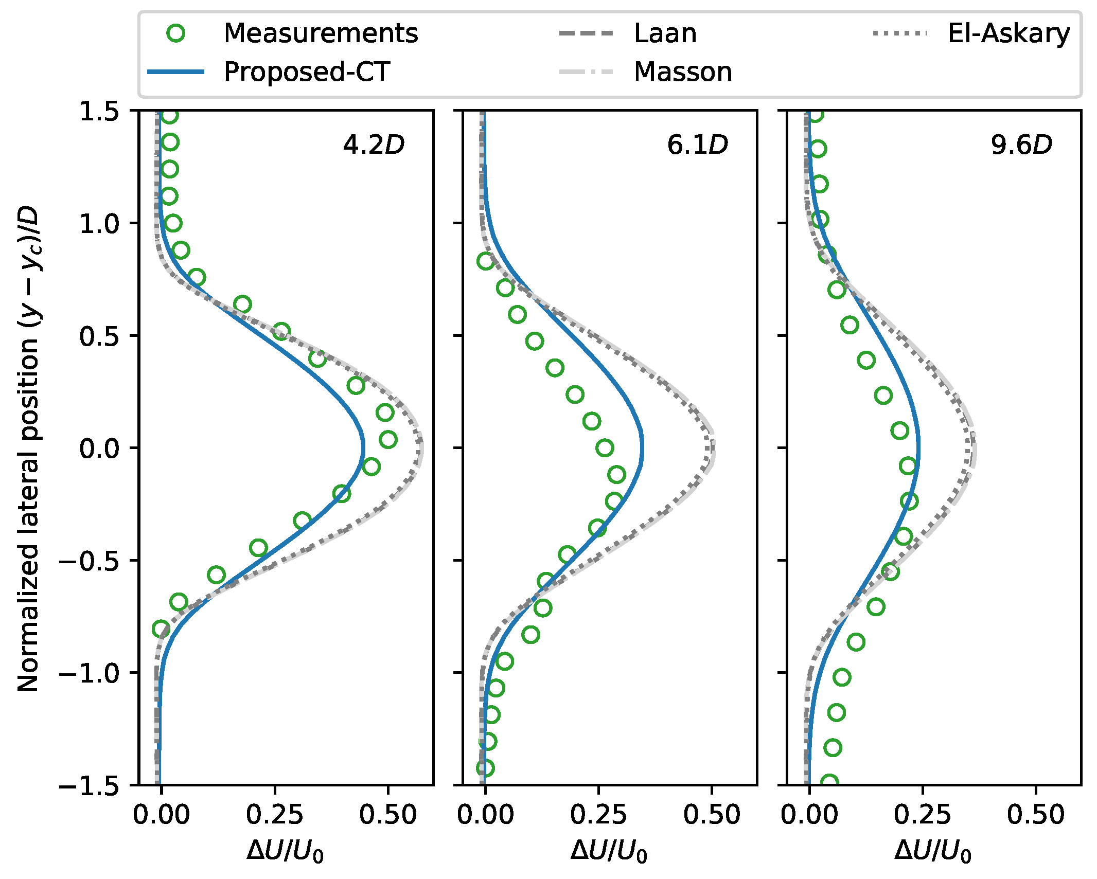
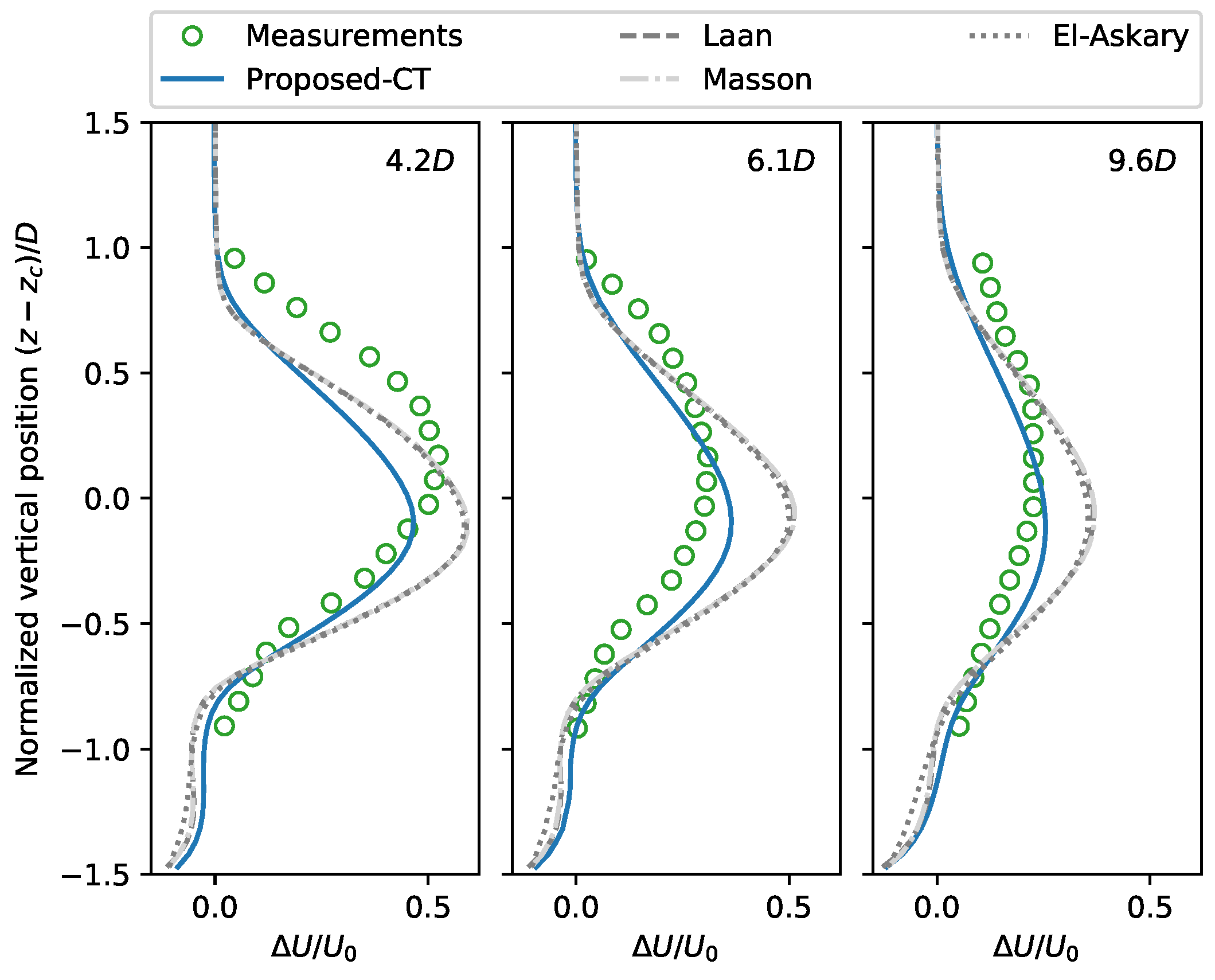
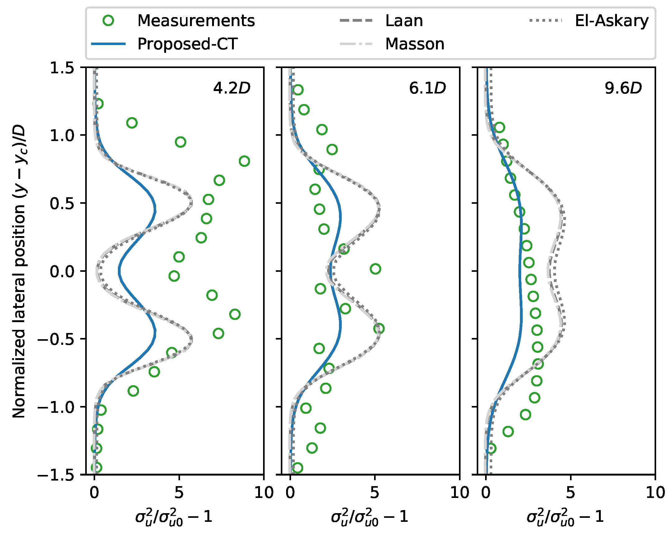
6.2. Case 2: Wakes of Danwin 180 kW Wind Turbines

The numerical results of the turbulence models based on MOST and the proposed model based on the new similarity functions are compared with the experimental data reported by Magnusson et al. [6] in Figure 15, Figure 16 and Figure 17. A comparison is made at distances 4.2, 6.1, and 9.6D downstream of the turbine. As the detailed rotor geometry of the Danwin 180 kW wind turbine is not available, the actuator disk model based on the thrust coefficient is applied.

Figure 15 and Figure 16 demonstrate the change of the wake deficit with the distance downstream of the turbine in both lateral and vertical directions. From this figure, it can be depicted that there is no discernible difference between AM, El-Askary, and Laan models at all downstream positions. As compared to measurements, these models that are based on MOST, predict larger wake deficits, and the wake deficit can be overestimated by 0.25 at 6.1D downstream of the rotor. Introducing the new similarity functions into the Laan model improves the wake prediction at 6.1D and 9.6D downstream, as compared with the models based on MOST. Note that the measured wake center or the position of the maximum wake deficit, shifts ~0.2D in both vertical and lateral directions at 6.1D and 9.6D downstream of the rotor. This shift of the wake center was also observed in full-scale turbine wakes with scanning-LiDAR measurements from the Crop Wind Energy eXperiment (CWEX) in Iowa [57]. The stretching of the wake structures can be attributed to the strong wind veer associated with stable conditions [6,57]. As wind veer is a direct result of Coriolis effects caused by the Earth’s rotation and the Coriolis force is not modeled in this work, all the test models fail to capture this stretching of the wake structures.

Figure 17 shows the distribution of the normalized added turbulence ${\sigma }_u^2/{\sigma }_{u0}^2-1$ in the lateral direction at hub height, where ${\sigma }_u$ and ${\sigma }_{u0}$ is the standard derivations of wind speed in wakes and in the atmosphere, respectively. A dual-peak pattern (lateral distance $y-y_c=\pm 0.5$D) is detected experimentally at 4D downstream of the rotor, as a result of rotor tip vortices and high shear production of turbulent kinetic energy caused by strong velocity gradients at the wake boundary [3,4]. All test models capture this dual-peak pattern with lower values: the measured peaks reduce by 3 in the simulations using models based on MOST and reduce by 5 in the simulations using the proposed model. This underestimation of the added turbulence may be due to representing the turbine rotor with actuator disk instead of the actual rotor geometry. Note that the dual-peak pattern predicted by the models based on MOST can be observed at distance downstream of the rotor up to 9.6D, which becomes indistinctly at 6.1D and 9.6D downstream of the rotor for both measurements and the simulations using the proposed model. As compared to measurements, the models based on MOST also overestimate the normalized added turbulence which is improved by the proposed model at 6.1D and 9.6D downstream of the rotor.

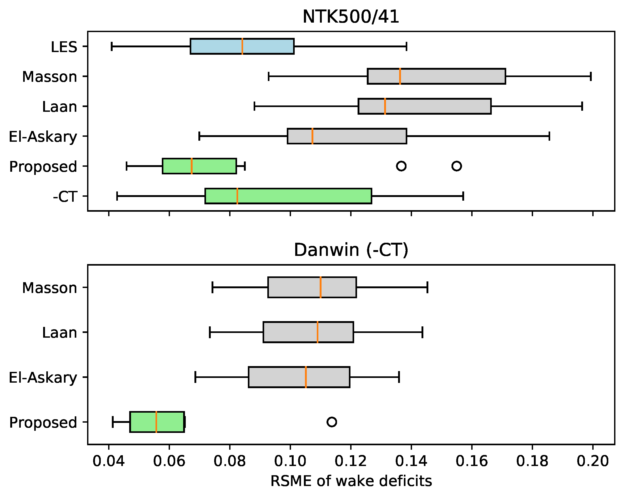
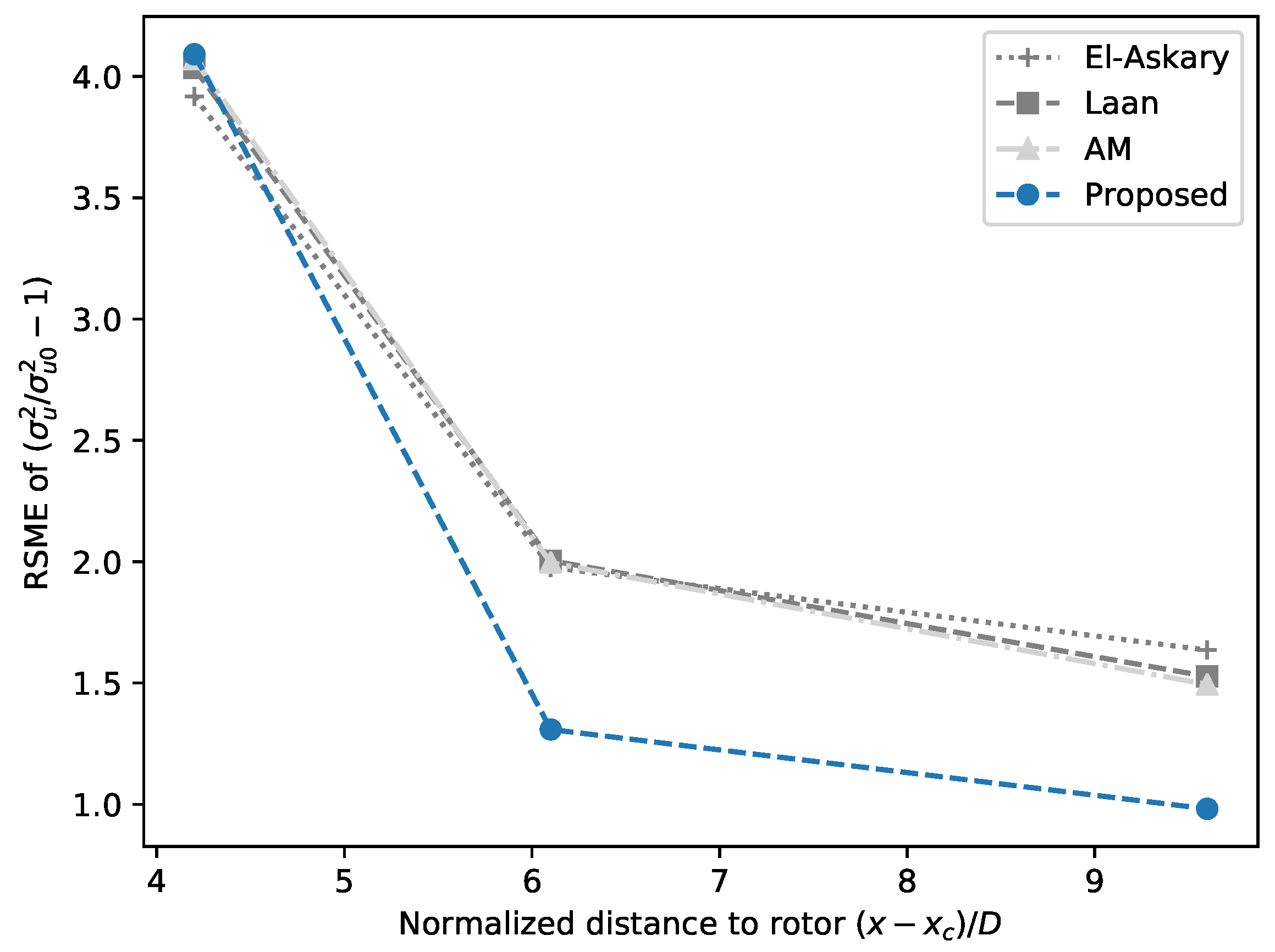
6.3. Model Assessment

In this section, we adopt the root-mean-square error (RSME) to analyze the accuracy of the CFD predictions using various turbulence models [58]:

$$\mathrm{RSME}=\sqrt{\frac{{\sum }_1^n{(y_{\mathrm{CFD}}-y_{\mathrm{EXP}})}^2}{n}}$$

(47)

where n is the number of measurement points in the evaluation, $y_{\mathrm{EXP}}$ is the experimental data, and $y_{\mathrm{CFD}}$ is the simulated values from CFD. Note that measurement points out of the wake range are not applied to calculate the RSME, and the wake width is set 2D due to wake simulations.

The RMSE analysis of the wake deficit is presented in Figure 18 and Figure 19. Over a range of 0.04 to 0.2, the lower the RSME value, the better the behavior of the numerical model. According to Figure 18, it can be depicted that the proposed model, either based on BEM in Case 1 or based on the thrust coefficient in Case 2, has the best performance with the lowest RMSE values, except for 4–5D in Case 1. The AM, El-Askary, and Laan models have similar performance in the wake prediction, but the El-Askary model has lower RMSE values among the various turbulence models based on MOST. As compared to AM and Laan model, the El-Askary model could reduce the RSME of the lateral wake deficit by 0.03 in Case 1 and 0.01 in Case 2. However, this improvement is smaller than that of the proposed model: introducing the new similarity functions into the Laan model could reduce the RSME of the lateral wake deficit by 0.05 averagely (Figure 18). The LES approach presented in Machefaux et al. [1] predicts a decreased RSME of the lateral wake deficit with the distance downstream of the rotor. Note that all test models, except for the LES approach, have poor performance in predicting wake structure at $5D$ downstream of the rotor. This could be a result of the downslope terrain or uncertainties due to LiDAR measurements [1].

Using BEM to distribute force through the rotor significantly improves near wake prediction at 1–3D downstream of the rotor in Case 1: the RSME of vertical wake deficit predicted by the proposed model using BEM approach is lower, 0.02–0.05, than the proposed model using the $C_T$ approach. However, it should be noted that the proposed model using $C_T$ approach has a similar performance in the wake prediction with that using BEM approach at $4D$–$5D$ downstream of the rotor. This suggests that the distribution of the momentum source through the rotor only affects near wake structures up to $3D$ and that one can expect similar accuracy of wake prediction for far wake regardless of which method to distribute the force through the rotor.

The RMSE analysis of the added turbulence is presented in Figure 20. The RMSE of the added turbulence is observed to decrease with the distance downstream the rotor. Turbulence intensities are significantly underpredicted at $4.2D$, where the RMSE of the added turbulence is ~4. More than $4.2D$ the RMSE of the added turbulence predicted by the proposed model is lower by 30% than those of models based on MOST. This indicates that introducing the new similarity functions into the Laan model can eliminate the side effects of the breakdown of MOST on wake modeling.

7. Conclusions

In this paper, the breakdown of MOST is investigated experimentally, and its side effects on wake modeling through numerical simulations are also investigated. New similarity functions based on a field measurement in a wind farm are proposed and applied in a turbulence model to eliminate the side effects of the breakdown of MOST on wake modeling. Wake simulations of two types of turbines under different stability conditions are carried out and compared with measurements from a LiDAR and cup anemometers. The main findings are as follows. (1) Field measurements show that MOST overestimates velocity gradient for $\zeta >0.1$ in the full range of $R_f$. The proposed similarity functions can limit the velocity gradient as the stability increases. (2) Due to the breakdown of MOST for $\zeta >0.1$, the test models based on MOST overestimate wake effects in both wake deficits and the added turbulence under stable conditions. (3) The new similarity functions constrain velocity gradient for $\zeta >0.1$ as compared with MOST, and introducing the new similarity functions into the Laan model improves the wake prediction under stable conditions. (4) By distributing the blade force through the rotor, momentum effects of the rotor to the atmospheric boundary layer are simulated in a more detail way than the uniformly distributed blade force applied based on the thrust coefficient. This enables the proposed model to capture the double-bell near-wake shape.

References

1. Machefaux, E.; Larsen, G.C.; Koblitz, T.; Troldborg, N.; Kelly, M.C.; Chougule, A.; Hansen, K.S.; Rodrigo, J.S. An experimental and numerical study of the atmospheric stability impact on wind turbine wakes. Wind Energy 2016, 19, 1785–1805. [Google Scholar] [CrossRef]
2. Han, X.; Liu, D.; Xu, C.; Shen, W.Z. Atmospheric stability and topography effects on wind turbine performance and wake properties in complex terrain. Renew. Energy 2018, 126, 640–651. [Google Scholar] [CrossRef]
3. Chamorro, L.P.; Porté-Agel, F. Effects of Thermal Stability and Incoming Boundary-Layer Flow Characteristics on Wind-Turbine Wakes: A Wind-Tunnel Study. Bound.-Layer Meteorol. 2010, 136, 515–533. [Google Scholar] [CrossRef] [Green Version]
4. Zhang, W.; Markfort, C.D.; Porté-Agel, F. Wind-turbine wakes in a convective boundary layer: A wind-tunnel study. Bound.-Layer Meteorol. 2013, 146, 161–179. [Google Scholar] [CrossRef]
5. Hancock, P.; Zhang, S.; Pascheke, F.; Hayden, P. Wind tunnel simulation of a wind turbine wake in neutral, stable and unstable wind flow. J. Phys. Conf. Ser. 2014, 555, 012047. [Google Scholar] [CrossRef]
6. Magnusson, M.; Smedman, A.S. Influence of atmospheric stability on wind turbine wakes. Wind Eng. 1994, 18, 139–152. [Google Scholar]
7. Iungo, G.V.; Porté-Agel, F. Volumetric lidar scanning of wind turbine wakes under convective and neutral atmospheric stability regimes. J. Atmos. Ocean. Technol. 2014, 31, 2035–2048. [Google Scholar] [CrossRef]
8. Menke, R.; Vasiljević, N.; Hansen, K.S.; Hahmann, A.N.; Mann, J. Does the wind turbine wake follow the topography? A multi-lidar study in complex terrain. Wind Energy Sci. 2018, 3, 681–691. [Google Scholar] [CrossRef] [Green Version]
9. Wu, Y.T.; Porté-Agel, F. Atmospheric turbulence effects on wind-turbine wakes: An LES study. Energies 2012, 5, 5340–5362. [Google Scholar] [CrossRef]
10. Xie, S.; Archer, C.L. A numerical study of wind-turbine wakes for three atmospheric stability conditions. Bound.-Layer Meteorol. 2017, 165, 87–112. [Google Scholar] [CrossRef]
11. Wu, Y.T.; Porté-Agel, F. Large-eddy simulation of wind-turbine wakes: Evaluation of turbine parametrisations. Bound.-Layer Meteorol. 2011, 138, 345–366. [Google Scholar] [CrossRef]
12. Keck, R. A Numerical Investigation of Nacelle Anemometry for a HAWT Using Actuator Disc and Line Models in CFX. Renew. Energy 2012, 48, 72–84. [Google Scholar] [CrossRef]
13. Prospathopoulos, J.M.; Politis, E.S.; Rados, K.G.; Chaviaropoulos, P.K. Evaluation of the Effects of Turbulence Model Enhancements on Wind Turbine Wake Predictions. Wind Energy 2011, 14, 285–300. [Google Scholar] [CrossRef]
14. El-Askary, W.; Sakr, I.; AbdelSalam, A.M.; Abuhegazy, M. Modeling of Wind Turbine Wakes under Thermally-Stratified Atmospheric Boundary Layer. J. Wind Eng. Ind. Aerodyn. 2017, 160, 1–15. [Google Scholar] [CrossRef]
15. Alinot, C.; Masson, C. kvarepsilon Model for the Atmospheric Boundary Layer Under Various Thermal Stratifications. J. Sol. Energy Eng. 2005, 127, 438–443. [Google Scholar] [CrossRef]
16. Van der Laan, M.P.; Kelly, M.C.; Sørensen, N.N. A new k-epsilon model consistent with Monin–Obukhov similarity theory. Wind Energy 2017, 20, 479–489. [Google Scholar] [CrossRef]
17. Grachev, A.A.; Andreas, E.L.; Fairall, C.W.; Guest, P.S.; Persson, P.O.G. The critical Richardson number and limits of applicability of local similarity theory in the stable boundary layer. Bound.-Layer Meteorol. 2013, 147, 51–82. [Google Scholar] [CrossRef]
18. Van Der Avoird, E.; Duynkerke, P.G. Turbulence in a katabatic flow. Bound.-Layer Meteorol. 1999, 92, 37–63. [Google Scholar] [CrossRef]
19. Foken, T. 50 years of the Monin–Obukhov similarity theory. Bound.-Layer Meteorol. 2006, 119, 431–447. [Google Scholar] [CrossRef]
20. Schlichting, H.; Gersten, K. Boundary-Layer Theory; Springer: Berlin/Heidelberg, Germany, 2016. [Google Scholar]
21. Launder, B.E.; Spalding, D.B. The numerical computation of turbulent flows. Comput. Methods Appl. Mech. Eng. 1990, 3, 269–289. [Google Scholar] [CrossRef]
22. Businger, J.A.; Wyngaard, J.C.; Izumi, Y.; Bradley, E.F. Flux-profile relationships in the atmospheric surface layer. J. Atmos. Sci. 1971, 28, 181–189. [Google Scholar] [CrossRef]
23. Dyer, A. A review of flux-profile relationships. Bound.-Layer Meteorol. 1974, 7, 363–372. [Google Scholar] [CrossRef]
24. Koblitz, T.; Sørensen, N.N.; Bechmann, A.; Sogachev, A. CFD Modeling of Non-Neutral Atmospheric Boundary Layer Conditions; DTU Wind Energy: Lyngby, Denmark, 2013. [Google Scholar]
25. Shen, W.Z.; Mikkelsen, R.; Sørensen, J.N.; Bak, C. Tip Loss Corrections for Wind Turbine Computations. Wind Energy 2005, 8, 457–475. [Google Scholar] [CrossRef]
26. Drela, M. XFOIL: An analysis and design system for low Reynolds number airfoils. In Low Reynolds Number Aerodynamics; Springer: Berlin/Heidelberg, Germany, 1989; pp. 1–12. [Google Scholar]
27. Du, Z.; Selig, M. A 3-D Stall-Delay Model for Horizontal Axis Wind Turbine Performance Prediction. In Proceedings of the 1998 ASME Wind Energy Symposium, Reno, NV, USA, 12–15 January 1998; p. 21. [Google Scholar]
28. Shen, W.Z.; Zhu, W.J.; Sørensen, J.N. Actuator Line/Navier–Stokes Computations for the MEXICO Rotor: Comparison with Detailed Measurements. Wind Energy 2012, 15, 811–825. [Google Scholar] [CrossRef]
29. Glauert, H. Airplane propellers. In Aerodynamic Theory; Springer: Berlin/Heidelberg, Germany, 1935; pp. 169–360. [Google Scholar]
30. El Kasmi, A.; Masson, C. An extended k–ε model for turbulent flow through horizontal-axis wind turbines. J. Wind Eng. Ind. Aerodyn. 2008, 96, 103–122. [Google Scholar] [CrossRef]
31. Grachev, A.A.; Andreas, E.L.; Fairall, C.W.; Guest, P.S.; Persson, P.O.G. On the turbulent Prandtl number in the stable atmospheric boundary layer. Bound.-Layer Meteorol. 2007, 125, 329–341. [Google Scholar] [CrossRef]
32. Pedersen, T.F.; Dahlberg, J.Å.; Busche, P. ACCUWIND-Classification of Five Cup Anemometers According to IEC 61400-12-1; Forskningscenter Risoe: Roskilde, Denmark, 2006. [Google Scholar]
33. IEC. 61400-12-1: Wind Turbines—Part 12-1: Power Performance Measurements of Electricity Producing Wind Turbines; IEC: Geneva, Switzerland, 2005. [Google Scholar]
34. Lira, A.; Rosas, P.; Araújo, A.; Castro, N. Uncertainties in the estimate of wind energy production. In Proceedings of the Energy Economics Iberian Conference—EEIC, Lisboa, Portugal, 4–5 February 2016; pp. 4–5. [Google Scholar]
35. Coquilla, R.V.; Obermeier, J. Calibration Uncertainty Comparisons between Various Anemometers; American Wind Energy Association: Washington, DC, USA, 2008. [Google Scholar]
36. Lindelöw-Marsden, P.; Pedersen, T.F.; Gottschall, J.; Vesth, A.; Wagner, R.; Paulsen, U.; Courtney, M. Flow Distortion on Boom Mounted Cup Anemometers; Risø-R-Report-1738 (EN); DTU Wind Energy: Lyngby, Denmark, 2010. [Google Scholar]
37. Högström, U. Non-dimensional wind and temperature profiles in the atmospheric surface layer: A re-evaluation. In Topics in Micrometeorology. A Festschrift for Arch Dyer; Springer: Berlin/Heidelberg, Germany, 1988; pp. 55–78. [Google Scholar]
38. Nieuwstadt, F.T. The turbulent structure of the stable, nocturnal boundary layer. J. Atmos. Sci. 1984, 41, 2202–2216. [Google Scholar] [CrossRef]
39. Dyer, A.; Hicks, B. Flux-gradient relationships in the constant flux layer. Q. J. R. Meteorol. Soc. 1970, 96, 715–721. [Google Scholar] [CrossRef]
40. Paulson, C.A. The mathematical representation of wind speed and temperature profiles in the unstable atmospheric surface layer. J. Appl. Meteorol. 1970, 9, 857–861. [Google Scholar] [CrossRef]
41. Coppin, P.; Bradley, E.F.; Finnigan, J. Measurements of flow over an elongated ridge and its thermal stability dependence: The mean field. Bound.-Layer Meteorol. 1994, 69, 173–199. [Google Scholar] [CrossRef]
42. Liang, J.; Zhang, L.; Wang, Y.; Cao, X.; Zhang, Q.; Wang, H.; Zhang, B. Turbulence regimes and the validity of similarity theory in the stable boundary layer over complex terrain of the Loess Plateau, China. J. Geophys. Res. Atmos. 2014, 119, 6009–6021. [Google Scholar] [CrossRef]
43. Grachev, A.A.; Andreas, E.L.; Fairall, C.W.; Guest, P.S.; Persson, P.O.G. SHEBA flux–profile relationships in the stable atmospheric boundary layer. Bound.-Layer Meteorol. 2007, 124, 315–333. [Google Scholar] [CrossRef]
44. Sorbjan, Z. An examination of local similarity theory in the stably stratified boundary layer. Bound.-Layer Meteorol. 1987, 38, 63–71. [Google Scholar] [CrossRef]
45. Blackadar, A.K.; Tennekes, H. Asymptotic similarity in neutral barotropic planetary boundary layers. J. Atmos. Sci. 1968, 25, 1015–1020. [Google Scholar] [CrossRef]
46. Tennekes, H. The logarithmic wind profile. J. Atmos. Sci. 1973, 30, 234–238. [Google Scholar] [CrossRef]
47. Bak, C.; Fuglsang, P.; Sørensen, N.N.; Madsen, H.A.; Shen, W.Z.; Sørensen, J.N. Airfoil Characteristics for Wind Turbines; Forskningscenter Risoe: Roskilde, Denmark, 1999. [Google Scholar]
48. Johansen, J.; Sørensen, N.N. Aerofoil characteristics from 3D CFD rotor computations. Wind Energy Int. J. Prog. Appl. Wind Power Convers. Technol. 2004, 7, 283–294. [Google Scholar] [CrossRef]
49. Vignaroli, A. UniTTe–MC1-Nordtank Measurement Campaign (Turbine and Met Masts); DTU Wind Energy: Lyngby, Denmark, 2016. [Google Scholar]
50. Magnusson, M. Near-wake behaviour of wind turbines. J. Wind Eng. Ind. Aerodyn. 1999, 80, 147–167. [Google Scholar] [CrossRef]
51. Zhang, X. CFD Simulation of Neutral ABL Flows; DTU Wind Energy: Lyngby, Denmark, 2009. [Google Scholar]
52. Sørensen, J.N.; Mikkelsen, R.F.; Henningson, D.S.; Ivanell, S.; Sarmast, S.; Andersen, S.J. Simulation of wind turbine wakes using the actuator line technique. Philos. Trans. R. Soc. A Math. Phys. Eng. Sci. 2015, 373, 20140071. [Google Scholar] [CrossRef] [Green Version]
53. Temel, O.; van Beeck, J. Two-equation eddy viscosity models based on the Monin–Obukhov similarity theory. Appl. Math. Model. 2017, 42, 1–16. [Google Scholar] [CrossRef]
54. Chang, C.Y.; Schmidt, J.; Dörenkämper, M.; Stoevesandt, B. A consistent steady state CFD simulation method for stratified atmospheric boundary layer flows. J. Wind Eng. Ind. Aerodyn. 2018, 172, 55–67. [Google Scholar] [CrossRef]
55. Weller, H.G.; Tabor, G.; Jasak, H.; Fureby, C. A tensorial approach to computational continuum mechanics using object-oriented techniques. Comput. Phys. 1998, 12, 620–631. [Google Scholar] [CrossRef]
56. Sørensen, N.N. General Purpose Flow Solver Applied to Flow Over Hills; DTU Wind Energy: Lyngby, Denmark, 1995. [Google Scholar]
57. Bodini, N.; Zardi, D.; Lundquist, J.K. Three-Dimensional Structure of Wind Turbine Wakes as Measured by Scanning Lidar. Atmos. Meas. Tech. 2017, 10, 2881–2896. [Google Scholar] [CrossRef]
58. Ntinas, G.K.; Shen, X.; Wang, Y.; Zhang, G. Evaluation of CFD Turbulence Models for Simulating External Airflow Around Varied Building Roof with Wind Tunnel Experiment; Building Simulation; Springer: Berlin/Heidelberg, Germany, 2018; Volume 11, pp. 115–123. [Google Scholar]
Figure 1. Schemtaics of the Blade Element Theory (BEM)-based actuator disk model.
Applsci 09 04256 g001
Figure 2. Complex terrain around M1, where Wind direction (WD) stands for the wind direction and D = 93 m is the diameter of wind turbine 14.
Applsci 09 04256 g002
Figure 3. Sketch (left) and physical appearance (right) of measurement setup for M1.
Applsci 09 04256 g003
Figure 4. Comparison of the wind speeds from sonic anemometers ( U s o n i c ) and cup anemometers ( U c u p ) for the wind direction in 0 ± 10 : measurements in symbols and fit curves in solid lines. r x y is the Pearson correlation coefficient.
Applsci 09 04256 g004
Figure 5. Plots of ϕ m as functions of ζ at 30 m above the ground level (AGL) for WD = 0 ± 10 .
Applsci 09 04256 g005
Figure 6. Plots of ϕ m of different models as functions of ζ : dots (measured data) and circles (bin-averaged measured data). n is the number of the measured data.
Applsci 09 04256 g006
Figure 7. Velocity profiles estimated based on different similarity functions ϕ m ( ζ ) (the upper part) and boxplots of errors of velocity predictions (the lower part). U e x p is the measured velocity in runs 3, 5, and 6, whereas U p r e d i c t is the value predicted at the corresponding height.
Applsci 09 04256 g007
Figure 8. Same as Figure 6 but for ϕ h of the north section.
Applsci 09 04256 g008
Figure 9. Performance curves of the NTK500/41 turbine.
Applsci 09 04256 g009
Figure 10. Compuational domain and meshing settings.
Applsci 09 04256 g010
Figure 11. Implementations of wake models in OpenFOAM where ϕ = ϕ / ζ , ϕ = 2 ϕ / ζ 2 for ϕ { ϕ k , ϕ m , ϕ ε } .
Applsci 09 04256 g011
Figure 12. Normalized velocity distribution at hub height under the stable condition, where large eddy simulation (LES) data are modified from Machefaux et al. [1], where ( x c , y c , z c ) is the center point of the disk, Δ U is the velocity deficit in the wake, and U 0 is the inlet velocity.
Applsci 09 04256 g012
Figure 13. Lateral wake deficit of a NTK500/41 wind turbine at hub height under the stable condition; Δ U is the velocity deficit in the wake and U 0 is the inlet velocity.
Applsci 09 04256 g013
Figure 14. Same as Figure 13 but for vertical wake deficit profiles.
Applsci 09 04256 g014
Figure 15. Same as Figure 13 but for Danwin 180 kW wind turbines. All turbulence models are combined with actuator disk model (AD) based on thrust coefficient.
Applsci 09 04256 g015
Figure 16. Same as Figure 15 but for vertical wake deficit profiles.
Applsci 09 04256 g016
Figure 17. Lateral added turbulence in wakes of Danwin 180 kW wind turbines at hub height under the stable condition; σ u and σ u 0 represent the standard derivations of wind speed in wakes and in the atmosphere, respectively. All turbulence models are combined with AD based on thrust coefficient.
Applsci 09 04256 g017
Figure 18. RSME of the wake deficit at hub height under the stable condition: “-CT” represents models using AD based on the thrust coefficient.
Applsci 09 04256 g018
Figure 19. Same as Figure 18 but for boxplots of the root-mean-squared error (RSME) of wake deficits.
Applsci 09 04256 g019
Figure 20. RSME of the lateral added turbulence in wakes of Danwin 180 kW wind turbines under the stable condition at hub height; σ u and σ u 0 represent the standard derivations of wind speed in wakes and in the atmosphere, respectively. All turbulence models are combined with AD based on thrust coefficient.
Applsci 09 04256 g020