Geographically Modeling and Understanding Factors Influencing Transit Ridership: An Empirical Study of Shenzhen Metro

Featured Application

Enriching the practical applications of direct demand models with geographically weighted regression (GWR) and examining the influencing factors of transit ridership can provide multiple potential implications for travel demand modelers, transit operators, and urban planners. The results of the GWR model indicate that transit travel demand (ridership) can be estimated by identifying the significant variables from a local perspective, which can help to establish an efficient transit system combined with sustainable urban development.

Abstract

Ridership analysis at the local level has a pivotal role in sustainable urban construction and transportation planning. In practice, urban rail transit (URT) ridership is affected by complex factors that vary across the urban area. The aim of this study is to model and explore the factors that impact metro station ridership in Shenzhen, China from a local perspective. The direct demand model, which uses ordinary least squares (OLS) estimation, is the most widely used method of ridership modeling. However, OLS estimation assumes parametric stability. This study investigates the use of a direct demand model on the basis of geographically weighted regression (GWR) to model the local relationships between metro station ridership and potential influencing factors. Real-world Shenzhen Metro smart card data are used to test and verify the applicability and performance of the model. The results show that GWR performs better than OLS estimation in terms of both model fitting and spatial interpretation. The GWR model demonstrates a high level of interpretability regarding the spatial distribution and variation of each coefficient, and thus can provide insights for decision-makers into URT ridership and its complex factors from a local perspective.

1. Introduction

The dramatic increase in urbanization in the last few decades has made urban rail transit (URT) a central pillar of public transport, due to its efficiency and transport capacity. Identifying the dynamic mechanisms of urban transit is critical to both infrastructure planning and transportation operation, and thus urban indicators such as URT station ridership must be investigated systematically and comprehensively. URT ridership is a key factor used to determine a station’s occupation in terms of space and the supporting facilities required. URT ridership is known to be affected by the interaction of specific urban elements (such as land use and socio-economics). Thus, understanding the impact of these elements is essential to accurately estimate travel demand and effectively plan and design urban systems, including planning infrastructure and deploying services and resources. URT ridership modeling can help estimate ridership and explore the influencing factors. The complex factors assumed to affect metro ridership include land use, socio-economics, intermodal transport accessibility, and network structures.

Ridership modeling has long been applied in the field of transportation planning. Numerous models have been developed to explore the relationships between transit ridership and influencing factors. The four-step model (generation, distribution, mode choice, and assignment) was first developed in the 1950s and has since been dominant in traffic analysis. However, the four-step model has various practical shortcomings, such as its low level of accuracy, imprecise data, insensitivity to land use, institutional obstacles, and high cost [1]. The model is more applicable to transit ridership estimation in traffic zones (large regions) than in stations (small detailed regions) [2]. The direct demand model has recently attracted attention as an alternative to the four-step model. This estimates ridership via regression models and treats it as a function of its influencing factors in the pedestrian catchment area (PCA) and can thus identify influencing factors that can help to increase the volume of transit ridership [1,3,4,5,6]. In the model, the PCA is the geographical area from which the station draws its passengers. The shape and size of the PCA are determined by the accessibility of one station and the distance from other stations to it. Buffers can be used to generate circular catchment areas with a given distance, and Thiessen polygons are typically used to define an area around each station, where every location is nearer to this station than to all the others. The main advantages of the direct demand model in ridership modeling are simple usage, easy interpretation, quick response, and low expenses. Ordinary least squares (OLS) multivariate regression is a commonly used direct demand model, and assumes that the parameters are stable [1,5,7,8,9,10,11,12,13,14,15,16]. The advantages of spatial models are considered in direct demand models, and thus provide a better spatial interpretation by implementing geographically weighted regression (GWR), which can measure the nonstationarity and heterogeneity of spatial parameters.

In addition, as real transportation systems are dynamic, the traffic demand of the transport network differs by the time of day and the day of week. The time-varying patterns of travel demand are accompanied by time-varying ridership, which is influenced by several factors. If the time dependence of travel demands is not considered, inaccurate estimations of ridership and incorrect analyses of the influencing factors may result. Thus, the specific factors influencing transit ridership at station level at different time periods should be identified so follow-up dynamic ridership forecasting can be accurately conducted, thus providing a theoretical foundation for real-time traffic management.

In summary, the current direct demand models have various shortcomings while the GWR model has various advantages in the modeling of latent spatially varying relations. Thus, a direct demand model based on the GWR model is used to model the factors affecting transit ridership during different periods (evening rush hours, nonrush hours, average weekday ridership, average weekend ridership, and average daily ridership per week). Feature selection is conducted via the backward stepwise method before the GWR process. The applicability and effectiveness of the framework are demonstrated using the Shenzhen Metro network as a case study. Ridership data for 118 Shenzhen Metro stations were collected using the Automated Fare Collection (AFC) system in 2013. Four types of potential factors are considered: land use, socio-economics, the accessibility of intermodal transport, and network structure information.

This study makes both methodological and empirical contributions, as follows. Methodologically, by quantifying the network structure factors using measurements in the domain of a complex network, comprehensive information and significant regression performance are obtained. To the extent of our knowledge, little research has been done in this way before. Empirically, different GWR models are implemented for different time periods, which can both model the local relationships between the metro station ridership and its potential influencing factors and interpret the temporal variation in the influencing factors of ridership. Therefore, the study contributes to metro planning and periphery development from both spatial and temporal perspectives. The findings also have several practical implications for urban and transport policymakers, thus bridging the gap between theory and practice. The study also advances the literature of transit ridership modeling from a local perspective. In addition, its framework can be extended to other areas, such as analyzing the influencing factors of public health conditions (virus and disease spreading) and customer volume at different locations.

The remaining parts of the paper are organized as follows. A comprehensive review of the research on modeling and analyzing transit ridership and its influencing factors is provided in Section 2. The data collected for the study are described in Section 3. Section 4 introduces the methods of estimating transit station ridership and identifying the key influential factors. Section 5 details and analyzes the results of the model implementation. Section 6 concludes and provides practical recommendations.

2. Prior Research

2.1. Models for Estimating Transit Ridership

Numerous studies have recently emerged that explore the influencing factors impacting transit ridership. We review the research focusing on direct demand models in transit ridership estimation (as summarized in

Table 1. A review of the literature related to transit ridership modeling [1,2,3,4,5,6,7,8,9,10,11,12,13,14,15,16,17,18,20,21,22,23,24,25,26,27,28,29].

City	Data Time Span	Response Variable									Factors Investigated										Analysis Method	Reference
		Average Weekday Ridership	Monthly Station Ridership	Annual Ridership	Residual Daily and Hourly Subway Ridership	Daily Station Passenger Volume	Morning Peak and Evening Peak Ridership	Weekly Ridership	Ridership by Transit Mode	Not Mentioned	Land Use	Network Structure	Intermodal Connections	Socio-Economics	Station Built Environment	Weather	Transit Service	Time	Citywide	External Connectivity
Seoul, Korea	Not mentioned	√									√		√							√	OLS/structural equation model (SEM)	Sohn and Shim (2010)
Madrid, Spain	2004		√								√	√	√								Distance-decay weighted regression	Gutiérrez et al. (2011)
Madrid, Spain	2004		√									√	√	√							OLS/GWR	Cardozo et al. (2012)
Nanjing, China	2010	√										√	√	√	√					√	OLS	Zhao et al. (2013)
Shanghai, China	2011					√					√	√	√	√							OLS	Pan et al. (2017)
Hong Kong; New York, U.S.	2005	√									√		√	√	√						OLS	Loo et al. (2010)
Nine U.S. cities (ranging from Buffalo to St. Louis to San Diego)	2000	√									√	√	√	√					√		OLS	Kuby et al. (2004)
The state of Maryland, which consists of 23 counties and the city of Baltimore, U.S.	2011					√					√			√	√		√				OLS	Liu et al. (2016)
Nanjing, China	2011						√				√		√		√						OLS and multiplicative regression	Zhao et al. (2014)
New York, U.S.	2010–2011				√											√					OLS	Singhal et al. (2014)
Singapore	Not mentioned						√				√							√			Decision tree (DT), support vector regression (SVR), and item-based collaborative filtering method based on cosine similarity (CF)	Hu et al. (2016)
Tokyo, Japan	2010	√									√			√	√						Back propagation neural network (BPNN)	Li et al. (2016)
Montreal, Canada	1998 and 2003	√					√				√			√							OLS	Chan and Miranda-Moreno (2013)
Beijing, China	2014							√			√			√							Cluster analysis	Deng and Xu (2015)
Seoul, Korea	Not mentioned									√	√		√	√							MGWR	Jun et al. (2015)
New York City, U.S.	Not mentioned	√												√	√						Network Kriging method	Zhang and Wang (2014)
265 urbanized areas in the U.S.	2000			√										√	√					√	Two-stage least squares regression (2SLS)	Taylor et al. (2003)
Jacksonville, Florida, U.S.	2001	√											√	√	√		√				Poisson regression	Chu (2004)
Bogota, Colombia	2005, 2006					√						√			√					√	2SLS	Estupiñán and Rodríguez (2008)
Seoul, Korea	2007								√		√				√		√				OLS	Sung and Oh (2011)
Seoul, Korea For	2010						√				√		√								Multiplicative and Poisson regression	Choi et al. (2012)
Broward County, FL, U.S.	2000			√							√			√			√				Negative binomial regression	Thompson et al. (2012)
Three major cities in Cyprus	Not mentioned	√												√		√	√	√		√	Multiplicative regression	Kepaptsoglou et al. (2017)
Shenzhen, China	2014					√					√		√	√							OLS/GWR	Tu et al. (2018)
Seven Latin American cities	2014	√									√		√	√			√			√	OLS	Vergel-Tovar and Rodriguez (2018)

). The most widely used direct demand model in this research field is OLS multiple regression. Kuby et al. (2004) [5], Sohn and Shim (2010) [8], Loo et al. (2010), Sung and Oh (2011) [10], Gutierrez et al. (2011) [1], Thompson et al. (2012) [11], Guerra et al. (2012) [12], Zhao et al. (2013) [13], Chan and Miranda-Moreno (2013) [14], Singhai et al. (2014) [15], Liu et al. (2016) [16], Pan et al. (2017) [17], and Vergel-Tovar and Rodriguez (2018) [18] all used OLS regression models to fit the relationship between transit ridership and its influencing factors. However, OLS regression is limited by its assumption that the factors affecting transit ridership have nothing to do with the spatial location of stations, as OLS regression does not consider the spatial autocorrelation of variables. Fotheringham (1996) [19] proposed the geographically weighted regression (GWR) model, which is able to reveal the spatial correlations of variables under the condition of spatial heterogeneity, and thus is more suitable for dealing with spatial data analytics.

GWR is widely used for spatial data analysis in many fields, such as economics, geography, and ecology. However, the model has rarely been applied to the field of transportation planning. The only analyses comparing the results of OLS and GWR modeling of the factors influencing transit ridership are those conducted by Cardozo et al. (2012) [2] and Tu et al. (2018) [20], who found a better fit for GWR. Jun et al. (2015) [21] used mixed geographically weighted regression (MGWR) models incorporating both local and global factors to explore the association between metro ridership and land use features. Their work provides new research directions that justify further investigations using this type of model. However, their GWR models still have some limitations, such as ignoring the differences in travel demand between time periods and other network structure factors. Thus, there is room for improvement in the implementation of GWR in transit ridership modeling.

Other methods have also been considered, such as multiplicative regression (Choi et al., 2012; Zhao et al., 2014; Kepaptsoglou et al., 2017) [3,22,23], two-stage least square regression (2SLS) (Taylor et al., 2004; Estupiñán and Rodriguez, 2008) [24,25], Poisson regression (Chu, 2004; Choi et al., 2012) [3,6], negative binomial regression (Thompson et al., 2012) [11], and structural equation modelling (SEM) (Sohn and Shim, 2010) [8]; geographical methods such as distance-decay weighted regression (Gutiérrez et al., 2011) [1] and the network Kriging method (Zhang and Wang, 2014) [26]; machine learning methods such as the decision tree (DT) and support vector regression (SVR); and item-based collaborative filtering methods based on cosine similarity (CF) (Hu et al., 2016) [27], cluster analysis (Deng and Xu, 2015) [28], and back propagation neural networks (BPNN) (Li et al., 2016) [29]. However, understanding the results is a major challenge in terms of the interpretability of the function modeled by the machine learning algorithm. In regression models, there is a very simple relationship between inputs and outputs, and thus we choose the GWR model for our study.

2.2. Explanatory and Response Variables

The explanatory variables used in the models summarized in Table 1 can be categorized into the four main groups of land use, socio-economics, transport accessibility, and network structure variables. Land use variables have been used extensively in previous research. For example, Jun et al. (2015) [21] first evaluated land use characteristics, including the proportions of residential, commercial and office, manufacturing, and mixed land use, within the PCAs of metro stations in the Seoul metropolitan area, and then explored the impact of these characteristics on metro station ridership. Hu et al. (2016) [27] examined the association between land use characteristics at two levels of granularity and public transit ridership in Singapore in time and space. The main socio-economics variables used are population, employment, and automobile ownership ratio. For example, Kuby et al. (2004) [5] identified the factors that attracted light-rail ridership in nine U.S. cities. They found that employment within walking distance of each station and residential population were significant factors. Thompson et al. (2012) [11] analyzed the determinants of work trip transit ridership in Broward County, Florida. Vehicles per person and parking fees were the potential determinants, and automobile parking fees were found to induce higher levels of transit ridership. As for the third category, transport accessibility, Loo et al. (2010) [9] considered the intermodal competition public transit mode (i.e., the number of bus stations within a station’s PCA) as an important factor influencing metro ridership, and they found that the number of bus stations is statistically significant in determining metro ridership in the regression model. Zhao et al. (2013) [13] studied how the accessibility of Nanjing metro stations to other modes of transport, such as feeder bus lines stopping at a station and park-and-ride spaces for nonmotor vehicles, influenced metro station ridership, and found that both were significant factors. Finally, in terms of network structure, Kuby et al. (2004) [5] considered transfer stations and terminal stations when examining the relationship between transit ridership and the station’s properties, using dummy variables to distinguish between these station types. Sohn and Shim (2010) [8] and Thompson et al. (2012) [11] also considered the factor of transfer station using dummy variables. However, measurements from graph theory and network analysis have not been applied in this research field, although practical significance can be achieved by calculating the degree centrality of nodes to distinguish between transfer, terminal, and normal stations, or by calculating a node’s betweenness centrality to indicate how a station allows traffic flows to pass from one part of the metro network to another.

In terms of the response variable in direct demand models, daily ridership has been the most common concern, as in Kuby et al. (2004) [5], Chu (2004) [6], Sohn and Shim (2010) [8], Loo et al. (2010) [9], Zhao et al. (2013) [13], and Zhang and Wang (2014) [26], who all regarded the average weekday ridership as the response variable. Gutierrez et al. (2011) [1] and Cardozo et al. (2012) [2] considered monthly station ridership as the response in their models. Taylor et al. (2003) [24] and Thompson et al. (2012) [11] used annual ridership as the response. Zhao et al. (2014) [22], Singhal et al. (2014) [15], Hu et al. (2016) [27], Li et.al. (2016) [29], and Chan and Miranda-Moreno (2013) [14] used the shorter hourly analysis interval (e.g., peak hour ridership) as the response. However, few studies have considered the differences in influencing factors between time periods.

3. Study Area and Data

Our study investigates Shenzhen Metro network, which consisted of five lines and 118 stations in the year of 2013. The Shenzhen Metro ridership used in this study was collected and aggregated from the transit entry-exit smart cards records between 14 October (Monday) 2013 and 20 October (Sunday) 2013, which are provided by Shenzhen Metro Corporation (Shenzhen Metro Corporation: http://www.szmc.net/) in China, which obtains the smart cards records from AFC system.

3.1. Explanatory Variables

Explanatory variables represent the factors that hypothetically affect the ridership at the station (

Table 2. Summary of explanatory variables.

Categories	Explanatory Variables	Acronym of Variables	Source	Minimum	Mean	Maximum
Land use (The number of ***(land uses) within PCA)	Residential units	Residence	Baidu Map	0	36.86	218
	Restaurants	Restaurant	Baidu Map	0	48.52	291
	Retailers/shopping	Shopping	Baidu Map	0	115.18	400
	Schools	School	Baidu Map	0	5.64	64
	Offices	Offices	Baidu Map	0	18.58	298
	Banks	Bank	Baidu Map	0	9.60	73
	Hospitals	Hospital	Baidu Map	0	1.008	10
	Hotels	Hotel	Baidu Map	0	13.24	135
Network structure	Distance to the city center	Dis_to_center	Calculated	0.36	9.97	27.41
	Degree centrality	Degree	Calculated	0.017	0.037	0.068
	Betweenness centrality	Betweenness	Calculated	0	0.11	0.31
Socio-economics	Population	Pop	Worldpop	27.54	156.49	354.55
	Days since opening	Days_open	UrbanRail	839	1762	3132
Intermodal transport accessibility	The number of bus stations within PCA	Bus	Baidu Map	0	7.72	30

). Variables can be categorized into four groups: (1) land use; (2) socio-economics; (3) network structure; (4) intermodal transport accessibility.

3.1.1. Land Use

Dovey et al. (2017) [30] believe that in large and medium-sized cities, friendly walking distance is generally 500 m. Therefore, we determine the PCA for each Shenzhen Metro Station as a circular buffer with a radius of 500 m. Then, with the help of Baidu Map API, we can collect the relevant data of land use variables. Land use variables include surrounding residence, recreational facilities, commercial districts, educational institutions, office areas, and so on. To be more detailed, land use variables involve the number of residential units, restaurants, schools, offices, hospitals, banks, shops, and hotels within the PCA with a radius of 500 m.

3.1.2. Socio-Economics

In the category of socio-economic variables, there are two factors to be considered. The information about when those metro stations were opened was collected from a website named

“UrbanRail” (Source: http://www.urbanrail.net/as/cn/shen/shenzhen.htm). With the information, we can calculate the elapsed days since stations were opened to the investigating days (14 October 2013 to 20 October 2013). A higher residential population is assumed to be positively correlated with ridership. Here, we obtained information on population distribution all around Shenzhen in 2013 collected from the website of Worldpop (Source: WorldPop (www.worldpop.org—School of Geography and Environmental Science, University of Southampton; Department of Geography and Geosciences, University of Louisville; Departement de Geographie, Universite de Namur) and Center for International Earth Science Information Network (CIESIN), Columbia University (2018). Global High Resolution Population Denominators Project—Funded by The Bill and Melinda Gates Foundation (OPP1134076). https://dx.doi.org/10.5258/SOTON/WP00645). The population data were processed with ArcGIS 10.2 (Environmental Systems Research Institute, Inc (Esri) (2014) Arcgis. URL http://desktop.arcgis.com/en/arcmap/). Specifically, the buffers of all stations with a radius of 500 m were generated and the population within the buffers are aggregated, and the population distribution and 500 m buffers are illustrated as Figure 1.

From Figure 1, we can observe that the densely populated areas are mainly surrounding the metro stations. The impact of residential population density on ridership in the buffer zone of each station will be analyzed in further modeling.

3.1.3. Network Structure

We consider the degree centrality, betweenness centrality, and the distance from metro stations to the city center as the main factors in the category of network structure. In graph theory and network analysis, degree centrality is one of the easiest centrality measures to calculate, which is simply a count of how many edges a node has. Betweenness centrality of a node is measured with the number of shortest paths (between any pair of nodes in the graphs) that passes through the target node [31]. Therefore, they are related to specific transfer stations, normal intermediate stations, and terminal stations, as well as the role of a station in allowing traffic flows to pass from one part of the metro network to the other. The city center of Shenzhen is Shenzhen Municipal People’s Government in Futian District. To accurately calculate the distance of each station to the city center, we take the influence of the radius of the earth into consideration, and the distance from station $i$ to the city center $Dis{t}_i$ is as follows (1):

$$Dis{t}_i=\mathrm{R}\ast \arccos \left(\cos \left(La{t}_0\right)\ast \cos \left(La{t}_i\right)\ast \cos \left(Lo{n}_0-Lo{n}_i\right)+\sin \left(La{t}_i\right)\ast \sin (La{t}_0\right))\ast \frac{\pi }{180}$$

(1)

where $\mathrm{R}$ is the radius of the earth, ($La{t}_0$, $Lo{n}_0)$ and ($La{t}_i$, $Lo{n}_i)$ are respectively the latitude and longitude of the city center and station $i$. The required geographical information was collected from Google Maps (Source: https://maps.google.com).

3.1.4. Intermodal Transport Accessibility

For intermodal transport accessibility, assuming that the number of surrounding bus stations of the metro station is positively correlated with the ridership at the station, we consider the feeder bus system of the metro. The data are also collected from the Baidu map.

3.2. Response Variable

The purpose of this study is to explore the various impact factors of metro station ridership during different time periods. As mentioned earlier, travel demands and patterns differ at the time of day and the day of week, and the temporal distribution of smart card records in all available days (14 October to 20 October) (shown in Figure 2b) indicates that the average daily travel frequency is higher than that on weekends.

We use the smart card records data collected from the AFC system of Shenzhen metro on 14 October 2013 to make a preliminary statistical analysis. Figure 2a presents the number of transaction records of smart cards distributed in space on 14 October. The top four stations (Grand Theatre Station, Laojie Station, Huaqiang Road Station, and Luohu Station) with the most transaction records are marked in Figure 2a.

Figure 2b shows the temporal distribution of smart card records. It is noted that there is a morning traffic rush and an evening traffic rush on both weekdays and weekends. Moreover, the records of rush hours on weekdays are significantly more than those of weekend rush hours, whereas the records of nonrush hours on weekdays are less than those of weekends.

Therefore, the regression models with different response variables including evening rush hour (17:00–19:00), nonrush hour (9:00–17:00, 19:00–23:00), average weekday ridership, average weekend ridership, and average daily ridership of a week (Shenzhen Metro is operated from 6:30 to 23:00 in 2013) are built to identify the impact factors of ridership during the five aforementioned time intervals. More concretely, ridership of each station is the sum of entry and exit records (Average daily ridership refers to the average of the total ridership within a few days of operation time (6:30–23:00). Evening rush hour ridership is determined by dividing the total ridership in the whole week of evening rush hours from 17:00 to 19:00 by 14 h (2 h multiplied by seven days). Nonrush hour ridership is obtained by dividing the total ridership of remaining time (9:00–17:00, 19:00–23:00) except morning (7:00–9:00) and evening rush hours of a whole week by 84 h (12 h multiplied by seven days)).

4. Methodology

4.1. Variable Selection

The structured data contain 14 explanatory variables (shown in Table 1) with a limited amount of observations, which may cause multicollinearity and overfitting. Redundant variables should be removed to ensure that the modeling process is efficient. Thus, before fitting the regression model, features from the original variables candidates must be selected. The backward stepwise regression method, a popular wrapper method, is used to select features and control the model complexity [32]. The regression begins with a full model with all variables included, and at each step the variables are gradually eliminated to minimize the specific statistic used as a variable selection criterion. We can thus eventually obtain a reduced model that best explains the data.

The Akaike information criterion (AIC) is commonly used in such methods. In general, suppose we have a model with variables. Let $p$ be the number of variables in the model. Then, the AIC values are as follows:

$$AIC=-2log-likelihood+2p$$

(2)

Models with more variables have smaller root sum squares (RSSs), indicating a better goodness of fit, but increasing the complexity with more parameters. Models that strike a balance between fit and model size can generalize the best and perform substantially better than others. The AIC penalizes large models, so it strikes a balance. Thus, we use the AIC as a selection criterion for the backward stepwise regression method to obtain a reasonable model.

4.2. Geographically Weighted Regression

We utilize geographically weighted regression (GWR) models to estimate station-level ridership. The GWR model is an extension of OLS multiple regression, which is shown as follows:

$$y_i=\beta +{\displaystyle \sum }_{k=1}^p{\beta }_k{x}_{ik}+{\epsilon }_i$$

(3)

Local parameters can be estimated by introducing a geographical location factor into the regression, and the extended GWR model is as follows:

$$y_i={\beta }_0\left(u_i,v_i\right)+{\displaystyle \sum }_{k=1}^p{\beta }_k\left(u_i,v_i\right)x_{ik}+{\epsilon }_i$$

(4)

where given the observation point $i\left(i=1,2,\dots ,n\right)$ with longitude/latitude coordinates $\left(u_i,v_i\right)$, $y_i$ and $x_{i1}$, $x_{i2}$, …, $x_{ip}$ refer to the observed values of the response variable $y$ and explanatory variables $x_1$, $x_2$, …, $x_p$ of point $i$, and ${\epsilon }_i$ is the error term, following a normal distribution. ${\beta }_k\left(u_i,v_i\right)$ $\left(k=1,2,\dots ,p\right)$ denotes $p$ unknown functions related to spatial location. The geographic location calibrated by $\left(u_i,v_i\right)$ of each observation point $i$ is weighted by the GWR model, and the weight is a type of distance decay function [33]. When calculating the distance matrix among stations, the Euclidean distance metric and network distance metric are assessed, and the latter considers that the travel activities always occur along the connection intermedia of the transportation network, such as metro lines and roads [26]. As the network structure of the Shenzhen Metro in 2013 was not particularly complex and there are no clear differences between the results calibrated by the network distance metric and the Euclidean distance metric, we use the Euclidean metric for simplicity of calculation. For application to other networks, the distance metric should be selected considering the network complexity, and more distance metrics related to network accessibility [34]. The determination of bandwidth will directly affect the weight function and the precision of the model, and is therefore critical. GWR4 software (GWR4 User Manual. http://geoinformatics.wp.st-andrews.ac.uk/download/software/GWR4manual.pdf.) is used to construct the GWR model, as it includes multiple kernel-type options and bandwidth methods. We select an adaptive bisquare kernel and use AICc to determine the bandwidth of the model, where AICc is the AIC with a correction for small sample sizes.

5. Results and Discussion

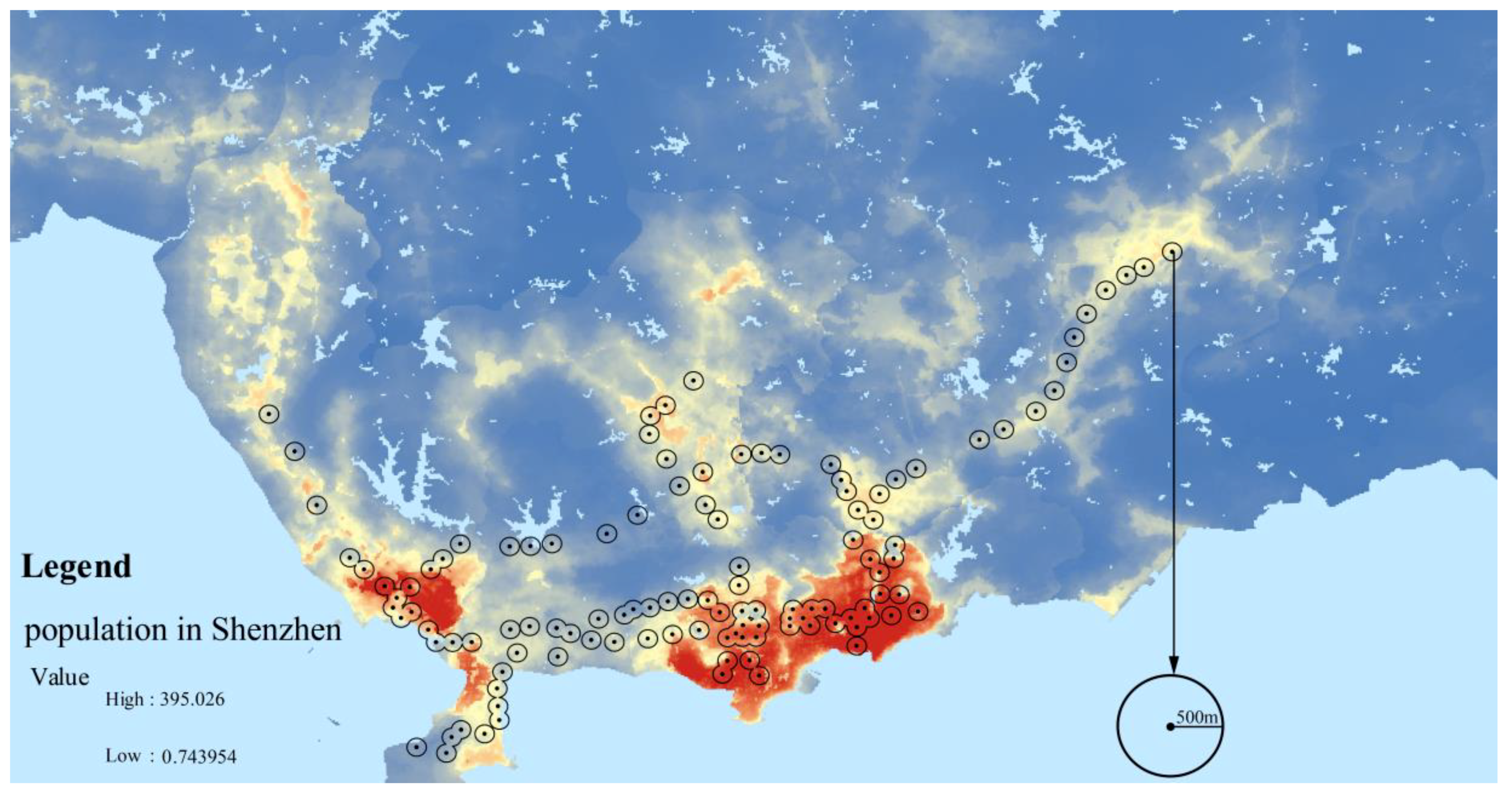
5.1. Spatial Autocorrelation Test for Variables

Establishing whether the candidate variables are spatially autocorrelated is necessary before the GWR model can be implemented. A spatial autocorrelation test can detect the degree of spatial correlation of the variables, which will provide theoretical support for the feasible application of spatial models. Moran’s I, proposed by Patrick Alfred Pierce Moran (1950) [35], is a correlation coefficient that measures the spatial autocorrelation. The estimated Moran’s I values of the response variables and all of the candidate explanatory variables are higher than the expected I values, indicating that the variables have positive spatial autocorrelations (

Table 3. Moran’s I test for spatial autocorrelation of all variables.

	Variable	Moran’s I	Expected I	p-Value
Response Variables	Weekly_ridership	0.241166216	−0.008547009	1.214e−06
	Weekday_ridership	0.263893648	−0.008547009	1.441e−07
	Weekend_ridership	0.166122759	−0.008547009	0.0004006
	Evenrush_ridership	0.277295727	−0.008547009	3.899e−08
	Nonrush_ridership	0.247797251	−0.008547009	4.637e−07
Candidate Explanatory Variables	Residence	0.393652311	−0.008547009	1.349e−14
	Restaurant	0.341715207	−0.008547009	1.692e−11
	Shopping	0.231551952	−0.008547009	3.923e−06
	School	0.289176791	−0.008547009	4.164e−11
	Offices	0.174946826	−0.008547009	1.365e−05
	Bank	0.388310167	−0.008547009	1.978e−14
	Bus	0.312294327	−0.008547009	7.898e−10
	Hospital	0.211271593	−0.008547009	1.263e−05
	Hotel	0.466480947	−0.008547009	<2.2e−16
	Dis_to_center	0.959152856	−0.008547009	<2.2e−16
	Degree	0.125833878	−0.008547009	0.005471
	Betweenness	0.241057563	−0.008547009	1.674e−06
	Pop	0.710332939	−0.008547009	<2.2e−16
	Days_open	0.383186771	−0.008547009	2.108e−13

). In the tables, we use the concise expressions weekly_ridership, weekday_ridership, weekend_ridership, evenrush_ridership, and nonrush_ridership to denote the average daily ridership in a week, average weekday ridership, average weekend ridership, evening rush hour ridership, and nonrush hour ridership, respectively. The Moran scatter plot can directly reflect the spatial autocorrelation of variables, and the plot has four quadrants. A strong positive spatial correlation is observed when the values are distributed in the first and third quadrants, and a negative spatial correlation will emerge if they fall in the second and fourth quadrants. Figure 3 presents the Moran scatter plots of several variables.

None of the Moran’s I values presented in Figure 3 are 0, indicating that they are not randomly distributed in space. In addition, most belong to the first and third quadrants, which indicates that the variables show significantly positive spatial autocorrelation. The three explanatory variables with the highest Moran’s I values are population, distance to the city center, and days since station opened, as their Moran’s I values are greater than 0.3 [36]. The results of the Moran’s I test thus provide a theoretical foundation for the rationale of the follow-up study.

5.2. Model Implementation and Results Analysis

Strong spatial autocorrelation is found for all of the variables included in our study. Thus, it is feasible to implement GWR models to explore the association between Shenzhen Metro ridership and its influencing factors. The final selection of explanatory variables derived from the backward stepwise regression method for the five models is given in

Table 4. Variables selected in the models.

Variables	Model 1	Model 2	Model 3	Model 4	Model 5
Response Variable (Ridership)	Weekly_ridership	Weekday_ridership	Weekend_ridership	Evenrush_ridership	Nonrush_ridership
Explanatory Variables	Pop	Pop	Pop	Pop	Pop
	Betweenness	Betweenness	Degree	Degree	Degree
	Days_open	Days_open	Betweenness	Betweenness	Betweenness
	Shopping	Office	Days_open	Days_open	Days_open
	Dis_to_center	Dis_to_center	Residence	School	Shopping
			Shopping	Dis_to_center	Dis_to_center

.

Table 4 enables us to find the common explanatory variables among the five models and the individual variables of each model. The common explanatory variables are the major factors impacting metro ridership, including population, betweenness centrality, and days since opening. The different individual variables of the five models indicate that factors affecting station-level ridership differ by the day of the week and time of the day.

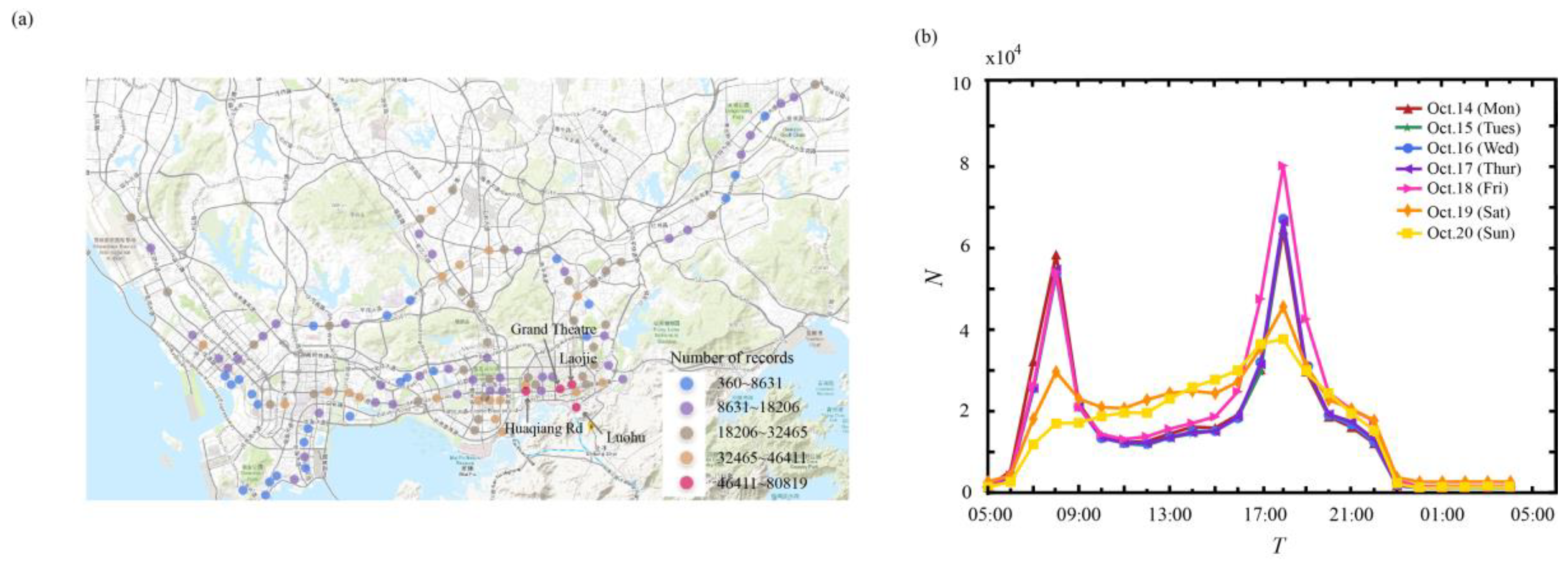
The number of offices within the PCA and the distance from the station to the city center are individual variables in the model for average weekday ridership. The number of residences and shopping places within the station catchment area is related to the average weekend ridership. Thus, commuting activities appear to mainly affect the average weekday ridership, while recreational activities related to commercial development such as shopping malls mainly affect the average weekend ridership. Across a single day, the number of schools and the distance to the center mainly affect the evening rush hour ridership, while the number of shopping places and the distance to the center mainly affect the nonrush hour ridership. Thus, passengers from schools (primary schools, high schools, and universities) contribute to the evening rush ridership and noncommuting activities like shopping affect the nonrush hour ridership.

Due to limitations on space, we only compare the results of Model 5 with those of the OLS model in

Table 5. Results of the model for Nonrush_ridership.

Global (OLS)						Local (GWR)
Variables	Estimate		Standard Error		t (Est/SE)	Min		Max		Mean		STD
Intercept	459.94		32.18		14.29	−1446.82		4350.79		519.97		792.78
Pop	118.36		39.43		3.00	−471.76		400.50		80.31		170.68
Degree	21.29		40.77		0.52	−200.12		340.02		57.51		149.68
Betweenness	48.65		42.70		1.14	−177.32		402.69		53.90		116.54
Days_open	135.09		33.90		3.98	−2116.29		2539.11		153.31		593.88
Shopping	53.01		35.73		1.48	−479.35		196.72		−20.25		152.92
Dis_to_center	−41.24		35.55		−1.16	−592.59		2590.58		55.57		447.78
Diagnostic
R-squared	0.33					0.88
Adjusted R-squared	0.29					0.77
Sigma	349.49					199.58
AICc	1727.10					1677.79
Residual sum of squares	13,557,658.86					2,475,111.14
Number of parameters	7					39.67
GWR ANOVA Table
Source		SS		DF			MS		F		p-Value
Global Residuals		1,355,7658.856		7.000
GWR Improvement		11,082,547.717		48.864			226,804.412
GWR Residuals		2,475,111.139		62.136			39,833.705		5.693781		0.0

, and we give the results of Models 1–4 compared with those of the OLS models in Appendix A (

Table A1. Results of the model for Weekly_ridership.

Global (OLS)						Local (GWR)
Variables	Estimate		Standard Error		t (Est/SE)	Min		Max		Mean		STD
Intercept	148,902.14		8373.14		17.78	−220,846.06		1,259,330.97		230,997.13		231,395.86
Pop	29,682.08		9949.31		2.98	−87,929.62		174,341.19		24,227.35		57,929.46
Betweenness	25,971.88		9096.29		2.86	−75,396.67		122,215.16		30,440.91		53,705.86
Days_open	36,322.47		8796.81		4.13	−449,460.34		868,771.29		72,348.20		158,603.43
Shopping	15,242.75		9217.93		1.65	−68,601.68		58,895.47		1474.80		29,877.34
Dis_to_center	−10,074.73		9248.92		−1.09	−207,415.70		755,777.31		43,828.83		157,781.05
Diagnostic
R-square	0.35					0.81
Adjusted R-square	0.32					0.65
Sigma	90,925.69					64,811.17
AICc	3038.33					3035.27
Residual sum of squares	925,957,952,739.49					269,172,991,697.74
Number of parameters	6					37.83
GWR ANOVA Table
Source		SS		DF			MS		F		p-Value
Global Residuals		925,957,952,739.493		6.000
GWR Improvement		656,784,961,041.749		47.919			13,706,255,804.666
GWR Residuals		269,172,991,697.743		64.081			4,200,487,280.123		3.263016		0.00000618

,

Table A2. Results of the model for Weekday_ridership.

Global (OLS)						Local (GWR)
Variables	Estimate		Standard Error		t (Est/SE)	Min		Max		Mean		STD
Intercept	21,354.89		1158.65		18.43	−57,334.43		148,479.18		23,875.86		28,629.01
Pop	4955.59		1297.64		3.82	−11,152.22		22,849.73		3284.89		7185.60
Betweenness	3932.25		1257.94		3.13	−7486.93		14,774.72		4679.16		5835.02
Days_open	4794.00		1199.76		3.99	−99,419.62		27,923.23		542.57		26,011.35
Working	632.51		1215.40		0.52	−8834.00		26,802.92		2937.24		8566.93
Dis_to_center	−1759.53		1295.76		−1.36	−24,571.36		86,428.59		4383.04		15,504.50
Diagnostic
R-square	0.37					0.79
Adjusted R-square	0.34					0.65
Sigma	12,582.09					9130.64
AICc	2571.58					2551.06
Residual sum of squares	17,730,610,368.11					5,947,129,532.95
Number of parameters	6					31.68
GWR ANOVA Table
Source		SS		DF			MS		F		p-Value
Global Residuals		17,730,610,368.116		6.000
GWR Improvement		11,783,480,835.168		40.665			289,772,173.512
GWR Residuals		5,947,129,532.948		71.335			83,368,605.017		3.475795		0.00000205

,

Table A3. Results of the model for Weekend_ridership.

Global (OLS)						Local (GWR)
Variables	Estimate		Standard Error		t (Est/SE)	Min		Max		Mean		STD
Intercept	21,069.11		1396.44		15.09	−120,163.53		88,286.30		15,756.13		34,442.86
Pop	3315.04		1641.47		2.02	−21,270.33		19,333.99		2360.82		7639.67
Degree	2650.45		1769.71		1.50	−10,861.88		21,766.31		4363.04		8529.63
Betweenness	2015.18		1776.54		1.13	−10,825.87		17,108.65		1367.15		5279.79
Days_open	5339.96		1475.52		3.62	−167,661.22		88,682.06		−281.66		41,401.46
Residence	1699.47		1726.48		0.98	−15,025.38		17,648.50		3450.52		6192.10
Shopping	2358.64		1754.75		1.34	−20,228.55		20,126.20		−497.87		7419.68
Diagnostic
R-square	0.29					0.86
Adjusted R-square	0.24					0.70
Sigma	15,165.28					9450.60
AICc	2616.89					2602.62
Residual sum of squares	25,528,398,304.96					5,143,828,231.09
Number of parameters	7					42.59
GWR ANOVA Table
Source		SS		DF			MS		F		p-Value
Global Residuals		25,528,398,304.956		7.000
GWR Improvement		20,384,570,073.869		53.407			381,681,908.043
GWR Residuals		5,143,828,231.087		57.593			89,313,770.481		4.273495		0.00000010

and

Table A4. Results of the model for Evenrush_ridership.

Global (OLS)						Local (GWR)
Variables	Estimate		Standard Error		t (Est/SE)	Min		Max		Mean		STD
Intercept	637.04		35.71		17.84	−2874.03		3506.87		640.77		957.13
Pop	148.58		40.39		3.68	−545.41		691.39		115.20		228.58
Degree	−26.14		44.94		−0.58	−356.74		372.09		−20.69		170.33
Betweenness	124.29		47.10		2.64	−173.17		583.86		178.10		186.16
Days_open	149.47		36.73		4.07	−4123.52		2067.64		43.21		952.39
School	45.76		35.97		1.27	−282.31		334.43		55.45		138.56
Dis_to_center	−57.96		39.57		−1.46	−1083.60		1956.09		114.93		433.65
Diagnostic
R-square	0.36					0.84
Adjusted R-square	0.32					0.70
Sigma	387.72					256.41
AICc	1751.60					1729.41
Residual sum of squares	16,686,678.25					4,226,169.97
Number of parameters	7					37.83
GWR ANOVA Table
Source		SS		DF			MS		F		p-Value
Global Residuals		16,686,678.255		7.000
GWR Improvement		12,460,508.283		46.718			266,718.092
GWR Residuals		4,226,169.972		64.282			65,744.115		4.056912		0.00000015

).

First, Table 5 shows that the AICc values of all of the GWR models are smaller than those of the corresponding global regression (OLS) models. According to the evaluation criterion proposed by Fotheringham et al. (1996) [19], if the difference between the AICc values of a GWR model and an OLS model is more than 3, the GWR model can be considered more applicable than the OLS model, even though it is more complex. The adjusted R-squared values of the GWR models are greater than those of the corresponding OLS models, demonstrating that the GWR model has strong explanatory power even when considering model complexity. Likewise, the parameter values (Sigma) indicating the model error of the GWR models are lower, and the residual sum of the squares from the GWR models are smaller than those from the OLS models. Thus, the results show that the GWR models generally perform better in goodness-of-fit measures than the OLS models. ANOVA tests, as shown in Table 5, are conducted to find out if the global (OLS) regression model and the GWR model have the same statistical performance (the same size of error variance). The results suggest that there is a significant improvement when GWR is used.

In addition, by comparing the results of the five models, the model for nonrush_hour ridership regression is found to perform the best in terms of the R-squared value. We only need the information about population distribution, degree centrality, betweenness centrality, days since opening, the number of shopping places and distance to the city center to use the GWR model to explain 88% of the response variable of nonrush hour ridership. In addition, the relevant data covering the information on the explanatory variables are easily accessible.

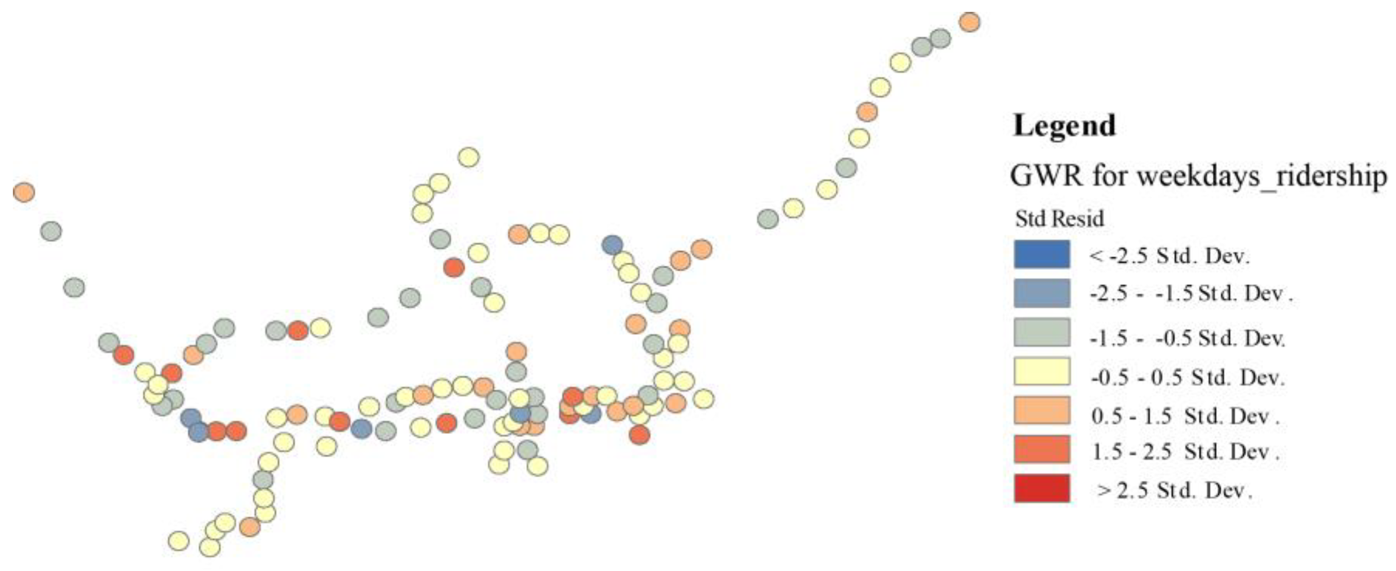
Figure 4 shows the standardized residuals of the GWR model for average weekday ridership, and for most stations these are relatively small, demonstrating the high accuracy of the model. Overpredictions (red bubbles) and underpredictions (blue bubbles) are randomly distributed in Figure 5, which indicates that our model is well specified. The spatial autocorrelation (Moran’s I) test of the regression residuals helps to ensure that they are spatially random (

Table 6. Global Moran’s I residuals test of the models for the average ridership across the whole week.

	OLS	GWR
Moran’s index	0.108184155	−0.114488799
Expected index	−0.008547009	−0.008547009
Variance	0.002855149	0.002870601
z-score	2.18460251	−1.9773379
p-value	0.01446	0.976

).

The global Moran’s I residuals test of the models for the average ridership over the whole week, shown in Table 6, demonstrates that GWR surpasses OLS, as the Moran I’s calculation is closer to the expected value in the GWR model. The residuals of the GWR model have a greater likelihood of random distribution (p-value) and show less variance (z-score). However, the residuals of OLS demonstrate statistically significant clustering characteristics (reflected by the Z-score and p-value).

The local indicator of spatial association (LISA) was proposed to represent local pockets of nonstationarity, assess the influence of individual locations on the magnitude of the global statistic, and identify “outliers” [37]. Figure 5 shows the LISA cluster maps of residuals in the OLS and GWR models for average daily ridership over a whole week. The residuals of the OLS model give significantly positive high-value clustering, while in the GWR model almost all of the clusters of residuals are ruled out, implying that GWR makes a significant improvement over OLS in terms of model fitting from the perspective of residuals.

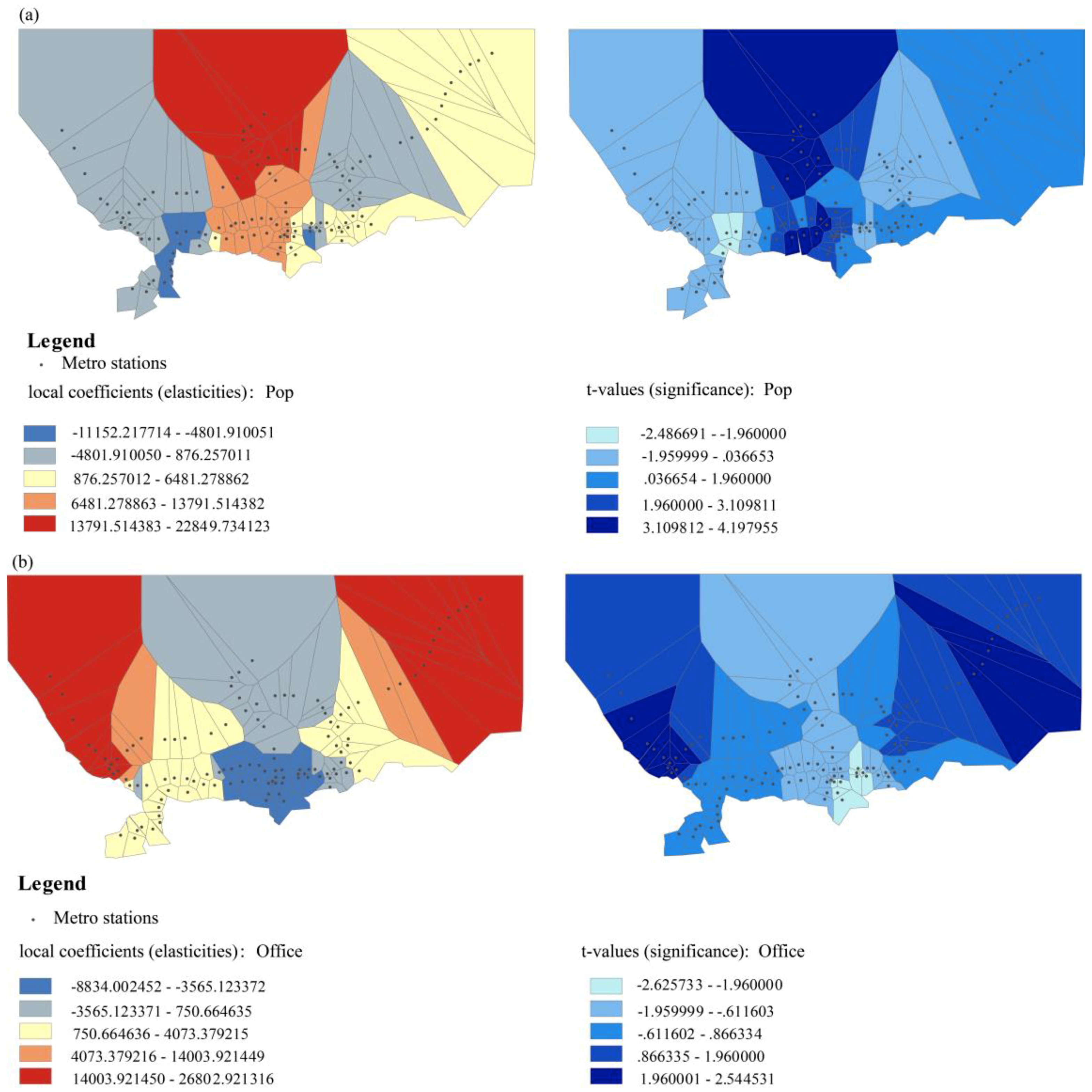
Using the Voronoi algorithm [38], the Shenzhen Metro coverage area can be divided into several Thiessen polygons according to the locations of the stations. Here, the spatial distribution of the local R-squared and local coefficients is visualized using Thiessen polygons. The values of the local R-squared range between 0 and 1, which indicates the satisfactory fitting of the local regression model. Mapping the local R-squared values can help us to see where GWR has a higher predictive capacity and where it performs poorly. Figure 6 illustrates the spatial distribution of the local R-squared of Model 2 for average weekday ridership and Model 5 for nonrush hour ridership, enabling us to understand where the model has a stronger explanatory power (local R-squared). Both Model 2 and Model 5 have a higher explanatory power in the central-north and southeast regions than in the other regions. In addition, the local R-squared values of most of the stations are higher than 0.82; these stations are mainly located in Luohu district.

By understanding the spatial distribution of local coefficients (elasticities) and t-values (significance), we can determine how the relationship between the variables changes spatially (estimated coefficients), and at what level of statistical significance. For example, in Model 2 (see Figure 7), as a common factor, the mean of the coefficients for the population variable is 3284.89. Thus, for each person within the station’s PCA, the number of trips adds up to 3284.89 each weekday. However, these elasticities are distributed unevenly in space. More trips per capita are expected in the central zone and the mid-north, where commercial and administrative areas and educational institutions are intensively distributed, while elasticity values are lower in the west and east. The t-value map on the right also shows that the effect of population is more significant in the middle area at a 0.05 level (the absolute value of a t-value larger than 1.96) (Figure 7a).

For the individually selected factor in Model 2, the mean of the elasticities for the office variable is 2397.24. Thus, for each new office within the station’s PCA, the number of trips adds up to 2397.24 each weekday. Elasticities are higher (more trips attracted per office) in the east and west than in the middle, whereas the elasticities of the central and north regions are negative and low, indicating that people who go to work in these regions depend more on transport other than the metro. In addition, the t-value map on the right shows that the effect of offices is more significant in the east, west, and mid-south areas at a 0.05 level (the absolute value is larger than 1.96) (Figure 7b). Thus, in general GWR is shown to have strong spatial explanatory power, based on local analysis of the variation of each coefficient across space (elasticities).

6. Conclusions

This study mainly discussed the impact factors of station ridership of Shenzhen metro at a local level during different time periods. Four categories of influencing factors, including land use, socio-economic, network structure, and intermodal transport access, are considered. For data collection of the factors of network structure, what is new compared with prior studies is that we introduce measurements from the field of network analysis, including degree centrality and betweenness centrality. Compared with the dummy variables mostly applied in the prior studies, these measurements covering comprehensive information can better quantify the network structure factors related to the practical significance of metro networks. Through adopting backward stepwise regression method for variables selection, and Moran’s I spatial autocorrelation test, this paper builds GWR models to analyze the influencing factors of Shenzhen metro ridership at different time resolutions (including the day of week and the time of day) during different time periods (average daily ridership of weekdays, weekends and a whole week, and average hourly ridership of evening rush hours and nonrush hours). Finally, we demonstrate the superiority of GWR models through the case study of Shenzhen metro. Additionally, the impact factors of Shenzhen metro station ridership are explored and analyzed from a local perspective.

The experimental results show that GWR models outperform OLS models in terms of both goodness-of-fit and explanatory power. In addition to the coefficient of determination of GWR models dramatically higher than OLS models, GWR models can provide more information about the spatial distribution of models’ elasticities and other parameters (e.g., significance and goodness-of-fit).

The main findings of this study can be summarized as follows. First, the influencing factors are not entirely consistent as time changes. For different models corresponding to different time periods, the common influencing factors including population, days since stations were opened, and betweenness centrality refer to the major impact factors of Shenzhen metro ridership, while the individual factors can help to address the different impact factors of Shenzhen metro ridership during different time periods. It is found that the main source of the ridership over weekdays is from the commuting, and the ridership is driven by recreational activities related to commerce such as shopping over weekends. In a day, the ridership during evening peak hours is mainly affected by activities from school and commutes, while the ridership at nonrush hours is mainly driven by recreational activities related to commerce. Second, the spatial distribution of elasticities can help us to identify where the specific factor can attract more trips, for example, more trips per capita are expected in the center and mid-north, where commerce, administration, and education are concentrated, while elasticity values are lower in the west and east of Shenzhen. These results of the GWR models show great spatial interpretation in transport planning.

Above all, these findings have significant implications for the understanding of transportation planning and periphery development. First, in general, population affects all metro station ridership, especially for the center and mid-north of Shenzhen, indicating that metro station ridership would be significantly increased by an additional resident population in these regions; therefore, the results suggest that it is reasonable to give priority to the planning and construction of the metro lines in the regions of densely distributed resident population. Second, betweenness centrality is positively associated with station ridership, indicating that the role of a station to the shortest paths through the metro network is important to attract more passengers, so it suggests the network planner take the network structure into consideration. Third, days since the stations were opened also has positive impacts on station ridership. One possible reason for this is that the first line of metro to be built is generally along the hottest line with the highest travel demands in a city. Therefore, it suggests those cities without metro and in the stage of metro system planning carry out forecasting and estimation of travel demands before determining the first line to be built. Fourth, traffic rush hours are different in different functional zones, so different strategies of diverting passenger flows are suggested to be adopted flexibly. For example, enhancing security when diverting passenger flows is vital in commercial developed areas, while improving transit efficiency is more important when diverting passenger flows in employment-based areas. Finally, the GWR model discusses different local effects of influencing factors on metro ridership. It implies that it is necessary for urban and transportation policy-makers to refer to the GWR results to adjust measures to local conditions when implementing the principle of Transit Oriented Development (TOD) planning.

In general, different GWR models implemented for different levels of time periods in this study can not only model the local relationships between the metro station ridership and its potential impact factors, but also interpret the temporal variation of impact factors of ridership, and therefore inspire metro planning and periphery development from both spatial and temporal perspectives.

This study was limited by the absence of some additional influencing factors and not incorporating the local model selection in the model. The method in this study could be extended to take the cross-boundary travel flows between Shenzhen and Hong Kong into consideration, which might have an impact on the ridership of cross-boundary metro stations (Luohu station as well as Futian Checkpoint station) [39,40]. It was not included in the present study because the data collection for the cross-boundary travel data involved the institutional barrier. We will extend the relevant study once the data are available. Moreover, future work will also be carried out on model improvement, and a GWR model incorporating regression coefficient shrinkage and local model selection would help us to gain more insights of metro planning and periphery development from a local perspective.

References

1. Gutiérrez, J.; Cardozo, O.D.; García-Palomares, J.C. Transit ridership forecasting at station level: An approach based on distance-decay weighted regression. J. Transp. Geogr. 2011, 19, 1081–1092. [Google Scholar] [CrossRef]
2. Cardozo, O.D.; García-Palomares, J.C.; Gutiérrez, J. Application of geographically weighted regression to the direct forecasting of transit ridership at station-level. Appl. Geogr. 2012, 34, 548–558. [Google Scholar] [CrossRef]
3. Choi, J.; Lee, Y.J.; Kim, T.; Sohn, K. An analysis of Metro ridership at the station-to-station level in Seoul. Transportation 2012, 39, 705–722. [Google Scholar] [CrossRef]
4. Cervero, R. Alternative approaches to modeling the travel-demand impacts of smart growth. J. Am. Plan. Assoc. 2006, 72, 285–295. [Google Scholar] [CrossRef]
5. Kuby, M.; Barranda, A.; Upchurch, C. Factors influencing light-rail station boardings in the United States. Transp. Res. Part A Policy Pract. 2004, 38, 223–247. [Google Scholar] [CrossRef]
6. Chu, X. Ridership Models at the Stop Level; Report No. BC137-31; National Center for Transit Research for Florida Department of Transportation: Tampa, FL, USA, 2004. [Google Scholar]
7. He, Y.; Zhao, Y.; Tsui, K.L. An Analysis of Factors Influencing Metro Station Ridership: Insights from Taipei Metro. In Proceedings of the IEEE Conference on Intelligent Transportation Systems (ITSC), Maui, HI, USA, 4–7 November 2018. [Google Scholar]
8. Sohn, K.; Shim, H. Factors generating boardings at Metro stations in the Seoul metropolitan area. Cities 2010, 27, 358–368. [Google Scholar] [CrossRef]
9. Loo, B.P.Y.; Chen, C.; Chan, E.T.H. Rail-based transit-oriented development: Lessons from New York City and Hong Kong. Landsc. Urban Plan. 2010, 97, 202–212. [Google Scholar] [CrossRef]
10. Sung, H.; Oh, J.T. Transit-oriented development in a high-density city: Identifying its association with transit ridership in Seoul, Korea. Cities 2011, 28, 70–82. [Google Scholar] [CrossRef]
11. Thompson, G.; Brown, J.; Bhattacharya, T. What Really Matters for Increasing Transit Ridership: Understanding the Determinants of Transit Ridership Demand in Broward County, Florida. Urban Stud. 2012, 49, 3327–3345. [Google Scholar] [CrossRef]
12. Guerra, E.; Cervero, R.; Tischler, D. The half-mile circle: Does it best represent transit station catchments. Transp. Res. Rec. 2012, 2276, 101–109. [Google Scholar] [CrossRef]
13. Zhao, J.; Deng, W.; Song, Y.; Zhu, Y. What influences Metro station ridership in China? Insights from Nanjing. Cities 2013, 35, 114–124. [Google Scholar] [CrossRef]
14. Chan, S.; Miranda-Moreno, L. A station-level ridership model for the metro network in Montreal, Quebec. Can. J. Civ. Eng. 2013, 40, 254–262. [Google Scholar] [CrossRef]
15. Singhal, A.; Kamga, C.; Yazici, A. Impact of weather on urban transit ridership. Transp. Res. Part A Policy Pract. 2014, 69, 379–391. [Google Scholar] [CrossRef]
16. Liu, C.; Erdogan, S.; Ma, T.; Ducca, F.W. How to Increase Rail Ridership in Maryland: Direct Ridership Models for Policy Guidance. J. Urban Plan. Dev. 2016, 142, 04016017. [Google Scholar] [CrossRef]
17. Pan, H.; Li, J.; Shen, Q.; Shi, C. What determines rail transit passenger volume? Implications for transit oriented development planning. Transp. Res. Part D Transp. Environ. 2017, 57, 52–63. [Google Scholar] [CrossRef]
18. Vergel-Tovar, C.E.; Rodriguez, D.A. The ridership performance of the built environment for BRT systems: Evidence from Latin America. J. Transp. Geogr. 2018, 73, 172–184. [Google Scholar] [CrossRef]
19. Fotheringham, A.S.; Brunsdon, C.; Charlton, M.E. Geographically Weighted Regression: A Method for Exploring Spatial Nonstationarity. Geogr. Anal. 1996, 28, 281–298. [Google Scholar]
20. Tu, W.; Cao, R.; Yue, Y.; Zhou, B.; Li, Q.; Li, Q. Spatial variations in urban public ridership derived from GPS trajectories and smart card data. J. Transp. Geogr. 2018, 69, 45–57. [Google Scholar] [CrossRef] [Green Version]
21. Jun, M.J.; Choi, K.; Jeong, J.E.; Kwon, K.H.; Kim, H.J. Land use characteristics of subway catchment areas and their influence on subway ridership in Seoul. J. Transp. Geogr. 2015, 48, 30–40. [Google Scholar] [CrossRef]
22. Zhao, J.; Deng, W.; Song, Y.; Zhu, Y. Analysis of Metro ridership at station level and station-to-station level in Nanjing: An approach based on direct demand models. Transportation 2014, 41, 133–155. [Google Scholar] [CrossRef]
23. Kepaptsoglou, K.; Stathopoulos, A.; Karlaftis, M.G. Ridership estimation of a new LRT system: Direct demand model approach. J. Transp. Geogr. 2017, 58, 146–156. [Google Scholar] [CrossRef]
24. Taylor, B.D.; Miller, D.; Iseki, H.; Fink, C. Analyzing the Determinants of Transit Ridership Using a Two-Stage Least Squares Regression on a National Sample of Urbanized Areas; UC Berkeley, University of California Transportation Center: Berkeley, CA, USA, 2003; Available online: https://escholarship.org/uc/item/7xf3q4vh (accessed on 1 September 2019).
25. Estupiñán, N.; Rodríguez, D.A. The relationship between urban form and station boardings for Bogotá’s BRT. Transp. Res. Part A Policy Pract. 2008, 23, 439–464. [Google Scholar] [CrossRef]
26. Zhang, D.; Wang, X.C. Transit ridership estimation with network Kriging: A case study of Second Avenue Subway, NYC. J. Transp. Geogr. 2014, 41, 107–115. [Google Scholar] [CrossRef]
27. Hu, N.; Legara, E.F.; Lee, K.K.; Hung, G.G.; Monterola, C. Impacts of land use and amenities on public transport use, urban planning and design. Land Use Policy 2016, 57, 356–367. [Google Scholar] [CrossRef]
28. Deng, J.; Xu, M. Characteristics of subway station ridership with surrounding land use: A case study in Beijing. In Proceedings of the ICTIS 2015-3rd International Conference on Transportation Information and Safety, Wuhan, China, 25–28 June 2015. [Google Scholar]
29. Li, J.; Yao, M.; Fu, Q. Forecasting Method for Urban Rail Transit Ridership at Station Level Using Back Propagation Neural Network. Discret. Dyn. Nat. Soc. 2016. [Google Scholar] [CrossRef]
30. Dovey, K.; Pafka, E.; Ristic, M. Mapping Urbanities: Morphologies, Flows, Possibilities, 1st ed.; Routledge: Abingdon, UK, 2017; pp. 154–156. [Google Scholar]
31. Kitsak, M.; Gallos, L.K.; Havlin, S.; Liljeros, F.; Muchnik, L.; Stanley, H.E.; Makse, H.A. Identification of influential spreaders in complex networks. Nat. Phys. 2010, 6, 888. [Google Scholar] [CrossRef]
32. Larose, D.T.; Larose, C.D. Data Mining and Predictive Analytics, 2nd ed.; John Wiley & Sons: New York, NY, USA, 2015; pp. 358–359. [Google Scholar]
33. Fotheringham, A.S.; O’Kelly, M.E.; O´Kelly, M.E. Spatial Interaction Models: Formulations and Applications; Kluwer Academic Publishers: Dordrecht, The Netherlands, 1989; pp. 112–115. [Google Scholar]
34. Curtis, C.; Scheurer, J. Planning for sustainable accessibility: Developing tools to aid discussion and decision-making. Prog. Plan. 2010, 74, 53–106. [Google Scholar] [CrossRef]
35. Moran, P.A. Notes on continuous stochastic phenomena. Biometrika 1950, 37, 17–23. [Google Scholar] [CrossRef]
36. Cressie, N. Statistics for spatial data. Terra Nova 1992, 4, 613–617. [Google Scholar] [CrossRef]
37. Amelin, L. Local Indicators of Spatial association-LISA. Geogr. Anal. 1995, 27, 93–115. [Google Scholar]
38. Tüceryan, M.; Jain, A.K. Texture Segmentation Using Voronoi Polygons. IEEE Trans. Pattern Anal. Mach. Intell. 1990, 12, 211–216. [Google Scholar] [CrossRef]
39. Wang, D. Hong Kongers’ cross-border consumption and shopping in Shenzhen: Patterns and motivations. J. Retail. Consum. Serv. 2004, 11, 149–159. [Google Scholar] [CrossRef]
40. Leung, A.; Burke, M.; Cui, J. The tale of two (very different) cities—Mapping the urban transport oil vulnerability of Brisbane and Hong Kong. Transp. Res. Part D Transp. Environ. 2018, 65, 796–816. [Google Scholar] [CrossRef]
Figure 1. The 500 m buffers of metro stations and population distribution.
Applsci 09 04217 g001
Figure 2. Spatiotemporal distribution of smart card records. (a) Spatial distribution of records on 14 October; (b) Temporal distribution of hourly records on different days of the week (14 October–20 October).
Applsci 09 04217 g002
Figure 3. Moran scatter plots of explanatory variables.
Applsci 09 04217 g003
Figure 4. Standardized residuals of GWR for average weekday ridership (Model 2).
Applsci 09 04217 g004
Figure 5. Local indicator of spatial association (LISA) cluster maps of residuals in the OLS and GWR models. Colors indicate significant positive (red and pink), negative (pale blue and yellow), and not significant (blue) spatial autocorrelation. (a) LISA cluster map of residuals of OLS model for the average ridership across the whole week. (b) LISA cluster map of residuals of GWR model for the average ridership across the whole week.
Applsci 09 04217 g005
Figure 6. Spatial distribution of the local R-squared values of Model 2 and Model 5. (a) Local R-squared values’ distribution of Model 2 (average weekday). (b) Local R-squared values’ distribution of Model 5 (nonrush hour).
Applsci 09 04217 g006
Figure 7. Spatial distribution of local coefficients (elasticities) on weekdays. (a) Spatial distribution of local coefficients (elasticities) and t-values (significance) for the population variable. (b) Spatial distribution of local coefficients (elasticities) and t-values (significance) for the office variable.
Applsci 09 04217 g007