Simulation of Metro Congestion Propagation Based on Route Choice Behaviors Under Emergency-Caused Delays

Featured Application

The findings of analyzing the spontaneous congestion propagation process under metro emergencies could provide valuable references for the metro operation departments to develop passenger control measures.

Abstract

Generally, metro emergencies could lead to delays and seriously affect passengers’ trips. The dynamic congestion propagation process under metro emergency-caused delays could be regarded as the aggregation of passengers’ individual travel choices. This paper aims to simulate the congestion propagation process without intervention measures under the metro emergency-caused delays, which is integrated with passengers’ route choice behaviors. First, using a stated preference survey data collected from Guangzhou Metro (GZM) passengers, route choice models are developed based on random regret minimization (RRM) theory under metro emergency conditions. Then, a simulation environment is established using graph cellular automata (graph-CA) with augmented GZM network structure, where an ASEIR (advanced susceptible-exposed-infectious-recovered) model with time delay is proposed as the evolution rule in graph-CA. Furthermore, considering passengers’ routing preferences, a quantified method for the congestion propagation rate is proposed, and the congestion propagation process on a subnetwork of the GZM network is simulated. The simulation results show that metro congestion during peak periods has a secondary increase after the end of the emergency-caused delays, while the congestion during nonpeak hours has a shorter duration and a smaller influence range. The proposed simulation model could clearly reflect the dynamic process of congestion propagation under metro emergencies.

1. Introduction

Metro emergencies such as power system breakdown, signal system failure, train malfunction and accidents caused by human factors (passengers and operators), are the main causes of the delays in the metro system. In most cases, the delays can easily lead to congestions in stations or sections, which could spread from one station (section) to another and congest the lines or even the entire metro network. Understanding the spontaneous congestion propagation process without intervention measures under metro emergency-caused delays, can be beneficial to obtain the influencing range and duration of the emergencies and provide metro operation department valuable references and decision-making basis in making passenger control measures. In other words, only if we understand how the congestion spread in the metro network under metro emergencies without passenger control measures, can we know when, where and how to reduce the impact of metro emergency-caused delays.

Generally, the congestion propagation process in the metro network can be regarded as the aggregation of passengers’ spontaneous route choice results, and their heterogeneities on route choices are vital factors influencing passenger flow distribution under metro emergencies in the entire metro network. In addition, due to the uncertainty and anxiety caused by the metro service disruptions, passengers’ route choice behaviors are dynamically changing and significantly different from the normal conditions, the state transfer process of all the stations and links in the metro network is also a dynamic process. However, the metro operators and relevant researchers are more accustomed to predicting metro passenger flow distribution just using the aggregated ridership data and ignoring passengers’ heterogeneity in route choices between metro emergency and normal conditions.

Therefore, this paper aims to simulate the congestion propagation process without intervention measures under metro emergency-caused delays, where the microscopic passengers’ route choice behaviors are integrated in order to quantify the congestion propagation rate of each metro station. In detail, based on a stated preference survey data and the random regret minimization (RRM) theory, the route choice model is developed to describe passengers’ preferences under the metro emergency-caused delays. Meanwhile, in order to get better understandings of the congestion propagation process, a dynamical simulation model is proposed, which is implemented with graph cellular automata (graph-CA) model and ASEIR (advanced SEIR, susceptible-exposed-infectious-recovered) model on Guangzhou metro (GZM) network. Furthermore, a quantified method for congestion propagation rate based on passengers’ routing preferences and ridership distributions is proposed and the simulation on a subnetwork of the GZM network is carried out as the empirical study.

The remaining part of this paper is organized as follows. Section 2 gives the literature review of relevant researches. Section 3 describes the route choice models with data, variables, methodology, and estimation results. Section 4 shows the congestion propagation process on the metro network under a graph-CA environment with the ASEIR model, where the simulation on the GZM network is made, then, the passengers’ routing preferences are integrated into the congestion propagation rate of the ASEIR model. Section 5 analyzes the congestion propagation process with an empirical study, and Section 6 presents the conclusions.

2. Literature Review

Along with continuously increasing travel demands, the scale of metro networks is also rapidly expanding. Hundreds of metro stations and sections inside the metro system, as well as the imbalanced distribution of passengers, have made metro emergencies occur more frequently than ever before. According to the statistics, 334 emergencies have been recorded in the Beijing subway system from 2014 to 2016 [1]. That is to say, a metro emergency occurs every three days on average, which will lead to serious impacts on passengers’ daily trips. Several studies related to metro emergencies have been carried out in recent years. The capacity of evacuating subway stations under emergencies is estimated by using a bi-level programming model, and the performance of a subway station has been calculated [2]. Big data methods are also used in analyzing the resilience and vulnerability of transit networks and provide measures and methodologies in planning and preparing for emergencies [3]. Additionally, a combined cause consequence analysis with the fuzzy causal model is proposed to analyze human factors (passengers and operators) in metro accidents, and an emergency of “passenger clamped by train doors” which is influenced by operator fatigue is found to happen at certain periods during the day [4].

Obviously, it is a clear signal that human factors’ influences in metro emergencies are taking as important elements in making intervention measures for metro operators. However, the existing researches are still just using the aggregated ridership data to predicate the passenger flow distribution and ignoring passengers’ heterogeneity in route choice preferences between metro emergency and normal conditions. Therefore, the mutual feedback mechanism between passengers’ route choices and the dynamic process of the congestion propagation in the entire metro network needs to be investigated, in order to provide much detailed information to the metro operators.

Fully understanding metro passengers’ route choice behaviors is the key to predict, simulate and control the massive ridership distributed in the metro network. The decision-making process has been investigated with the introduction of random utility maximization (RUM) theory since the 1970s [5,6], where the theory assumes that the rational decision-makers can always capable of perceiving the utilities of all the alternatives in the choice set and choosing the alternative with the highest utility. The RUM theory with its conciseness and achievable properties has been widely applied in researches of behavior analysis, where its linear-additive implementation (multinomial logit model, i.e., MNL model) is the most used tool for analyzing travel behaviors. However, despite its many advantages, the disadvantage of the MNL model is also distinguished that it is not sensitive to the changes in the choice set when the random term of the model function follows the identical and independent distribution, and it is called independence of irrelevant alternatives (IIA). Due to the IIA property in the MNL model, either the identical alternatives in the choice set will be treated as different options, or the changes in alternatives or attributes will not be reflected in the comparison between two alternatives, which will lead to failures in model calibration. While, this defect can be remedied with mathematical methods such as nested logit (NL) model, mixed logit model and latent class model (LCM). NL model performs like the multi-level MNL model, where the alternatives are divided into several nests and the IIA property is eliminated between the nests. As the RUM based NL model is preferable in most situations [7], Yang et al. [8] explored route choice behaviors of drivers driving battery-electric vehicles. The mixed logit model is defined as an MNL model with random coefficients drawn from a cumulative distribution function [9], which considers the unobserved heterogeneity by allowing parameters to be distinct from each individual. Nevertheless, the source of individual-related heterogeneity cannot be well explained in the mixed logit model, and the latent class model is proposed, where the decision-makers are divided into several latent classes in which their preferences for alternatives and attributes are assumed similar to each other [10].

The extensions of RUM models achieved plenty of results in analyzing travelers’ choice behaviors [11,12,13], but travelers trend to use various criteria to evaluate their best choices despite the widely used RUM models, and regret theory (RT) is more suitable to model passengers’ choice behaviors especially under certain conditions [14]. In RT, regret, the negative experience of choosing a worse option from a choice set, is the thing decision-makers want to minimize the most. Therefore, as a counterpart method to the RUM approach, the random regret minimization (RRM) method is established as a discrete choice paradigm based on RT [15,16]. The decision process is different in RUM and RRM, for the former one compares the utilities among alternatives in the choice set, while the latter one compares deeply into the attributes level between different alternatives. Empirical researches in travel choices [17,18], environmental and resource economics analysis [19], traffic accident avoidance [20], fuel consumption [21], and purchasing behaviors [22,23], indicate that with its non-linear function, the RRM approach performs better in avoiding IIA property, and shows better model fit in plenty of travel choice scenarios. In addition, the particular characteristics of RRM models, semi-compensatory property and compromise effect, give a new perspective on transportation policy suggestions.

Congestion propagation in the metro network is a dynamic process, influenced by passengers’ choices and network topological characteristics. As an abstract dynamic system and a useful tool in simulation, cellular automata (CA) plays an important role in discrete mathematics [24]. Have been developed for several decades, CA is capable of simulating complicated phenomena in physic, biology, and environmental sciences. Simplicity, flexibility, intuitiveness, and transparency are the distinguishing features of CA-based models, and the ability to integrate geographical information as well as the high spatial resolution with computational efficiency makes CA models a powerful tool for researchers [25]. CA models consist of four basic components: cells, cell space, a set of possible states for the cells, and the cell states’ evolution rules that are correlated with discrete time steps. Moreover, with the advancement in the CA concept and the improvement of computing capability, a growing number of CA models are applied to simulating urban systems. Li, Gao, et al. [26] investigated the characteristic behaviors of railway traffic flow with the CA model and realized the simulation of some complex phenomena like a go-and-stop wave and the complex behavior of train movement. Zheng, Xi, et al. simulated passengers’ behavior in the subway system using a dynamic parameter CA model, and simulated pedestrian flows in waiting, inbound and outbound behaviors [27].

The state of a cell in the CA is determined by the states of the neighborhood cells, and simple evolution rules can result in complicated system performances. Therefore, neighborhood relationships and evolution rules are the key points in simulating realistic phenomena. Relaxation methods to expand the neighborhood of restricting CA models include irregular cell space [28,29], non-uniform cell space, extended neighborhood [30] and non-stationary neighborhood [31]. Graph-CA is proposed as a method to relax the restrictions in cell neighborhoods, and its derivation both from a graph and from the formalism of CA makes it a useful generalization of the conventional CA models [32]. Martinez et al. [33] constructed a graph-CA model, which is combined with the epidemic propagation model, and simulated the spreading processes of a general epidemic. In the research that investigating surface flows in planes [34], the graph-CA model is established with the CA environment supported by a graph structure, and the simulation results show excellent agreement compared to the traditional models. In social networks [35], graph-CA is used to simulate the effectiveness of the recommendation system based on CA with the usage of dependency graphs obtained from social networking sites. Moreover, graph-CA is also applied to solve the problem of maximum lifetime coverage problem in wireless sensor networks [36]. A modification of graph-CA is made with a variable configuration of cells and relation-based neighborhoods have enabled the capability of modeling travel behaviors on road networks [37].

The evolution rules in CA models can be modified to reflect the changes of cell states, which is another method to relax the restrictions in traditional CA models. As passengers are traveling through the metro network, the propagation of the outburst passenger flow is obvious traveling with emergency influenced passengers. The propagation process could be described by propagation dynamics on the network, like the SIS model, SIR model, SEIR model, etc. In these models, the states are defined as susceptible (S), exposed (E), infectious (I) and recovered (R), where these state can change in a single direction from S to E, S to I, E to I, E to R, or I to R. The stations’ states in the metro network can be analogous to these states, where congested stations that could spread its passengers to other stations are in state I. Congested station inside its own without the ability to influences others are in state E. Stations that could be influenced by the metro emergency-caused delays are in state S. As well, those stations where passenger flow control measures have been implemented are “immune” to congestions are in state R. SIS model has been used to simulate propagations on hypergraph [38], and SEIRS model is investigated in scale-free networks [39].

To sum up, the existing researches are starting to put attention on the interactions between metro emergencies’ influences and passengers’ choice behavior. However, most of them are either confined to the purely behavioral analysis and fewer results are shown in application correlated with metro emergency-caused delays or limited to the traditional methods of passenger flow analyzing, and the congestion propagation on the metro network is neglected. Therefore, in the following part of this paper, the route choice models are developed, the estimation results are analyzed and integrated with the congestion propagation process under metro emergency-caused delays for a more accurate simulation.

3. Route Choice Modeling

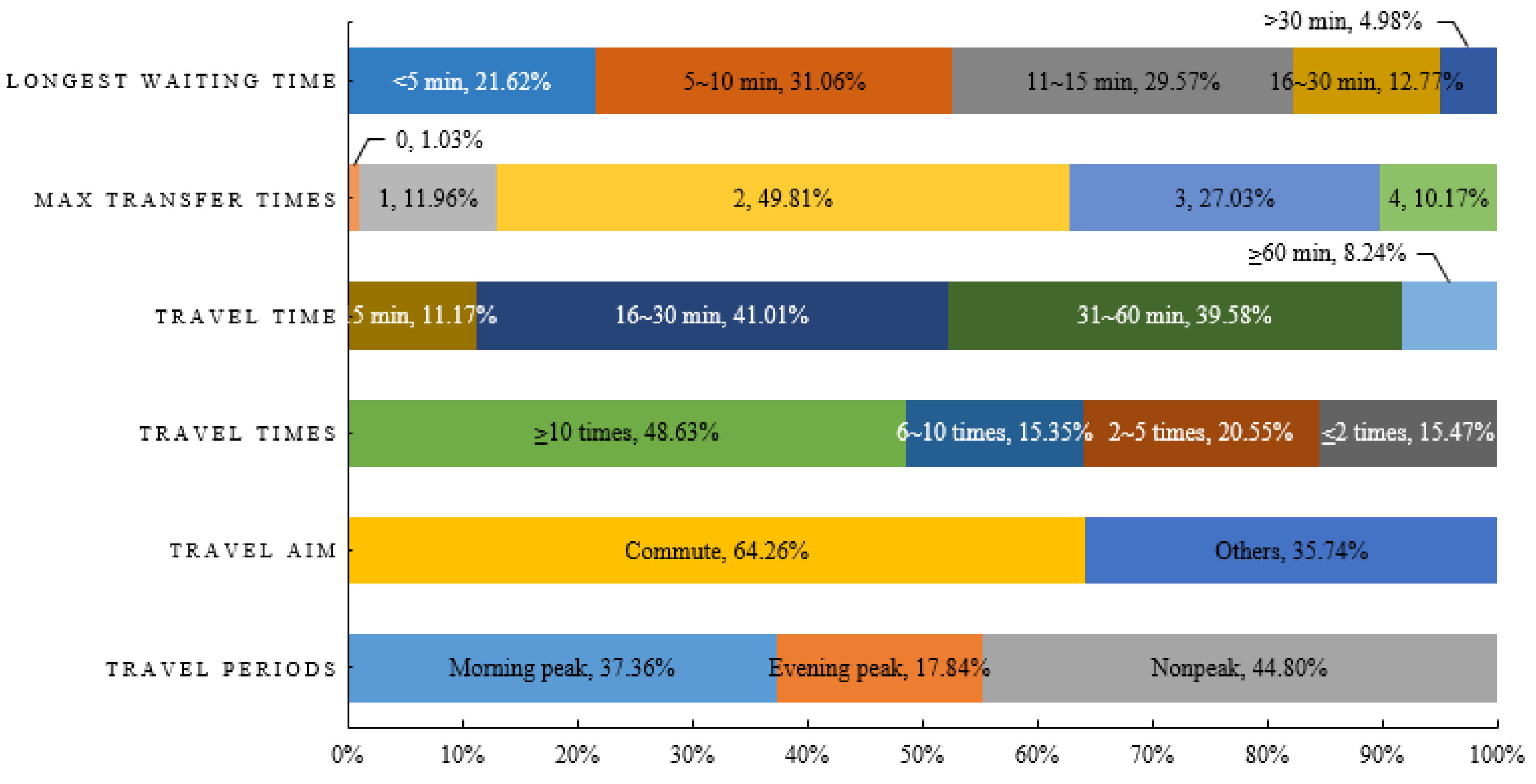
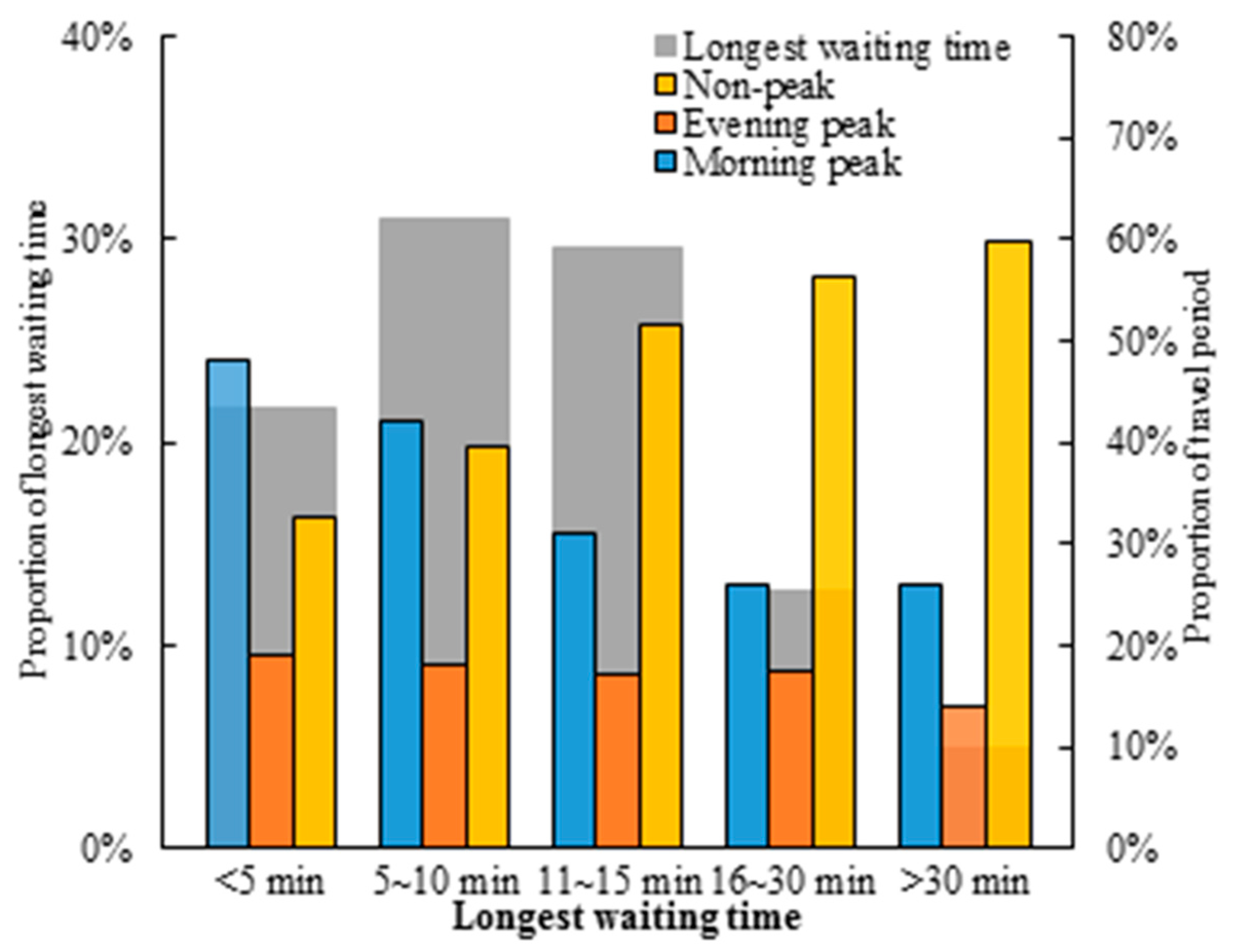
3.1. Data

GZM network is the urban rail transit system providing traffic service in Guangzhou and the Pearl River Delta area. By the end of 2018, GZM has 14 lines and 257 stations (including 31 transfer stations) in operation, and its operating mileage (478 km) ranks the third all around the world. The daily average ridership of the entire metro network of GZM is over 8 million, and during holidays or some large special events, the daily ridership can surpass 10 million.

Once the emergency occurs in the GZM network, the operators will estimate the delay time caused by the emergency based on their experiences and the delay information will be send out by official notice, broadcast and passenger information display system (PIDS), as shown in Figure 1. When the emergency-caused delay is less than 10 min, the information will be informed to the passengers on the line where the emergency occurs, when delay time is longer than 10 min and less than 30 min, passengers on adjacent lines will receive the delay information, once the delay time is over 30 min, all metro passengers on the GZM network will get the delay information. Moreover, when the normal operation is resumed, the information will be sent out by all measures so that all metro passengers could get relevant travel information and adjust their travel in time.

The analysis of metro passengers’ route choice behaviors under emergency-caused delays is based on the stated preference (SP) survey carried out in the GZM network. There are totally 6 scenarios in the questionnaire with different origins and destinations alongside with various combinations of route alternatives among multiple traffic modes like metro, bus, and taxi. The attributes of the routes are listed in the questionnaire and each respondent is asked to make their choices in 2 to 4 scenarios based on their travel experiences in the public transportation system, as show in

Table 1. Route properties in the survey.

Route	Traffic Mode	Route Property	Delay Time
1	Metro	The time shortest route before the metro emergency occurs.	3 to 20 min
2	Metro, metro & bus or taxi	Detour routes in metro alone or combined with ground traffic modes like bus or taxi, travel time is longer than route 1.	0
3			0
4			0
5	Bus	Passengers abandon the metro because of the emergency-caused delays and switch to ground traffic modes like buses or taxis. Travel time or travel cost may be higher than the metro routes.	0
6	Taxi		0

. After classification and collation of the collected questionnaires, 5520 are valid from 5553 questionnaires (10,128 valid samples can be used for further analysis).

Among the respondents who participated our survey, male accounts for 62.73% and female accounts for 37.27%, and most of them (94.38%) are younger than 45 years old, which is in line with the majority of metro passengers. Less than 3 transfer times in the metro network can be accepted by a larger proportion of metro passengers, and only about 10% of the passengers can bear 4 or more transfer times. About two-thirds of the metro travelers are commuting to work or school, and the proportion is in line with passengers whose weekly travel times over 6 times or more in the metro system. When a metro delay is inevitable, about 52% of the passengers can only endure waiting for less than 10 min. Other detailed attributes of the respondents of the SP survey is shown in Figure 2.

3.2. Explanatory Variables

Generally, many variables could influence passengers’ mode and route preferences under the delays caused by metro emergencies, such as route attributes, topological properties of the metro network and delay specific variable. In this study, route attributes such as travel time, travel cost and transfer time are taken into consideration.

The topological properties of the metro network are designed as indicators to evaluate the importance of stations and routes in the network. Passengers always prefer the fastest, shortest or the most convenient route between origin and destination and unwilling to take detours when the metro system is normally operating. However, when the chosen route is delayed by the emergencies, passengers may have to weigh between taking detours and waiting for the original route. Angular cost (AC) is the indicator designed to demonstrate passengers’ unwillingness about taking detours and the penalty of detoured routes. As metro routes do not directly connect origin and destination, especially when origin and destination are not on the same line. The deviation between the chosen metro routes and the direct connect of origin-destination have a significant influence on passengers’ route choices [40,41]. The angular cost increases with the increase of the deviation angles and the length of the route. Zhang et al. [42] modified the original formula by using the tangent function, as shown in Equation (1). With this modification, the AC is more sensitive to the changes in deviation angle and the impact on passengers’ route choice behaviors is more significant.

$$A{C}_k^{od}={\displaystyle \sum _s^{N_s}{L}_s\times \tan \frac{{\theta }_s}{4}}$$

(1)

where, route k’s AC from station o to station d is represented by ${\mathit{AC}}_k^{\mathit{od}}$, assume route k goes through N_s stations between o and d, and the section from station s to station s + 1 is represented by L_s, s ∈ S, where S is the set of stations in the metro network. The angular deviation between section s and the direct connection of o and d is represented by θ_s, θ_s ∈ [0, π].

Moreover, different metro stations play different roles in the network, and transfer stations and non-transfer stations may be valued differently for different passengers. Especially, when an emergency occurs in the metro system, a route with more transfer stations can offer more route alternatives than the ones with fewer transfer stations, but a transfer station always means more passengers and the station could be very crowded. The differences between stations are represented by station betweenness centrality (BC), which is the ratio between the amount of the shortest routes through the particular station and all the shortest routes in the network. BC derives from graph theory, and it measures metro stations’ importance by their ability to control the shortest routes. A station with higher BC means stronger control capability over the entire network, and if it is disabled by metro emergencies, all the shortest routes that go through this station have to stop operating [43,44]. In our research, we do not only focus our attentions on metro stations’ BC, but also consider the betweenness of the routes, and it can be calculated by the following equation:

$$B{C}_k={\displaystyle \sum _s^{N_s}b{c}_s}={\displaystyle \sum _s^{N_s}{\displaystyle \sum _{p\ne q\ne s}\frac{N_{pq}(s)}{N_{pq}}}}$$

(2)

where N_pq(s) is the amount of shortest routes between station p and station q that go through station s, N_pq is the total amount of shortest routes between p and q in the entire network, s, p, q ∈ S.

Apart from the aforementioned explanatory variables that describe characteristics of the routes and the networks, another explanatory variable is designed in this research to demonstrate the feature of emergency-caused delays, not just take the delay time as a variable. The conception of delay specific variable derives from the question that once the time shortest route is delayed by the metro emergencies, will the metro passengers choose to wait for the line to resume operation, or take detour routes, or just abandon metro and switch to other traffic modes? Moreover, under what conditions will the passengers choose to abandon their daily travel routes and which route will they pick to continue their travel? In order to quantify the influences of the emergency-caused delays, an indicator called route-switching cost (RSC) is designed. As can be seen in Equation (3), RSC is a penalty variable depicting the relative time cost if the passengers choose to switch their original route to other routes. It is assumed that all passengers tend to choose the time shortest route (i.e., route l) as their original route when there are no metro emergencies in the metro network, and once the emergency occurs, waiting or switching to other routes will lead to changes in the time cost.

$$RS{C}_k=\{\begin{array}{l}\exp \left(\frac{T_k-(T_l+D{T}_l)}{T_l}\right),k\ne l\\ 1,k=l\end{array}$$

(3)

where, RSC_k is the route switching cost of route k between a certain origin o and destination d; T_k and T_l is the travel time of route k and route l; DT_l is the delay time of route l, the time shortest route; k, l ∈ R_od, R_od is the set of available routes from o to d.

When the metro emergency occurs, if the travel time of route k is larger than the summation of travel time and delay time of route l, the time cost of route switching will be larger than 1, passengers may be unwilling to switch to route k. On the contrary, if the travel time of route k is lesser than the summation of travel time and delay time of the original shortest route l, then the relative time cost of switching route will be smaller than 1, and under this condition, switching route will be a wiser idea. Moreover, if passengers choose to wait for their original route to resume operation, the value of RSC will be equal to 1, which means that no penalty is attached to alternative l.

3.3. Model Description

RRM models are developed as a counterpart method to RUM models to avoid IIA property in the most widely used multinomial logit (MNL) model. As a discrete choice paradigm, the RRM model with its non-linear formulation provides us a new perspective to analyze the decision-makers’ (i.e., metro passengers’ in our research) routing behaviors under the delays caused by metro emergencies [15]. The core of RRM models lies in the postulation that when choosing from a set of alternatives, passengers are more concerned about reducing their regret, which derives from their chosen alternative perform worse than the nonchosen alternatives in terms of one or several attributes. In order to achieve this goal, passengers have to compare on the attribute level between every two alternatives in the choice set, rather than just comparing the utility of the alternatives, which is the choice mechanism of RUM models. Following this particular principle, the formula of random regret can be given by Equation (4):

$$R{R}_i=R_i+{\epsilon }_i={\displaystyle \sum _{j\ne i}{\displaystyle \sum _M\ln \left(1+\exp \left({\beta }_m(x_{jm}-x_{im})\right)\right)}}+{\epsilon }_i$$

(4)

where RR_i is the random regret generated from choosing alternative i; ε_i is the stochastic term referring to the unobserved factors that influence passengers’ choices; R_i is the random regret value calculated by the aforementioned explanatory variables. β_m is the attribute x_m’s parameter that needs to be estimated; x_im, x_jm are the values of attribute x_m of alternative i and alternative j, i, j belongs to the choice set C; M is the number of attributes in an alternative, m ∈ M.

The probability of each alternative in the RRM model can be specified by Equation (5):

$$\begin{array}{ll}\hfill P(i|C)& =P(R{R}_i<R{R}_j,\forall i,j\in C,i\ne j)\\ & =P(-R_i>-R_j)=\frac{\exp (-R_i)}{\exp (-R_i)+{\displaystyle \sum _{C,i\ne j}\exp (-R_j)}}\end{array}$$

(5)

The non-linear characteristic of the RRM model can be seen in Equation (4), and it is capable of describing the change of random regret. When β_m and x_jm − x_im are synchronously positive or negative, which means that if the attribute has a positive (negative) effect, but the chosen alternative i performs worse (better) than alternative j in this attribute, the regret will rise rapidly. Conversely, when the product of β_m and x_jm − x_im is negative, the random regret is pretty close to 0. It is because that if the attribute has a positive effect (β_m > 0) and alternative i outperforms alternative j (x_jm < x_im) in attribute x_m, passengers have already made a good choice and there is no need to regret anymore. Comparing with the linear-additive RUM model, the non-linear characteristic result in another two unique properties of RRM models, semi-compensate property and compromise effect. Semi-compensate property refers to the asymmetry on the changes of attributes’ values, in detail, the influence on the random regret of the increase (or decrease) of an attribute’s value could not be fully compensated by the changes of another attribute. That is, if the route has the shortest travel time but the highest travel cost, the advantage of travel time and the disadvantage of travel cost cannot offset each other. This property leads to the fact that alternative with more balanced attribute values rather than alternatives with obvious good and bad attribute values can achieve the smallest random regret, and that is the phenomenon of compromise effect.

3.4. Estimation Result

Apart from the explanatory variables above, the sensitivity of waiting time is another crucial factor when evaluating passengers’ choice preferences with emergency-caused delays. Obviously, the commuters could be more pleased to reduce their waiting time in their trip, while those who travel during the nonpeak period may be more unconcerned about the length of waiting time. This distinction of delay time perception is captured by our survey and is shown in Figure 3. Passengers traveling during morning peak periods are the most sensitive to waiting time, and as the waiting time increases, fewer people will be able to tolerate it. Evening peak period follows the same tendency that most of the metro passengers can endure 5 to 10 min delays, and, afterward, the number of passengers who willing to wait decreases with the waiting time extends.

However, during the nonpeak period, the tendency is exactly the opposite that the passengers’ acceptance of longer waiting time is much higher than peak periods. Moreover, as the longest waiting time extends, the proportion of the nonpeak period is monotonically increasing. It indicates that passengers that travel during the nonpeak period are more tolerant of longer waiting time than passengers who travel during peak periods.

The significantly different tendency about waiting time under different periods reflects passengers’ heterogeneity in route choices under metro emergencies. Therefore, apart from the route choice model that describes passengers’ routing behaviors of the entire day (M1), route choice models for peak periods (M2) and nonpeak periods (M3) are also estimated to investigate the detailed distinctions of passengers’ preferences under metro emergency-caused delays. The estimation results are listed in

Table 2. Estimation results of route choice models.

Models	Alternatives	M1	M2	M3
Parameters		Value (t-Test)	Value (t-Test)	Value (t-Test)
ASC1	Route 1	7.790 (114.770)	7.630 (83.200)	7.930 (77.080)
AC/m		0.178 (13.210)	0.167 (8.750)	0.190 (9.870)
BC		−0.204 (−3.890)	−0.143 (−1.950)	−0.273 (−3.630)
RSC		−0.059 (−5.460)	−0.076 (−3.400)	−0.049 (−3.900)
Travel cost/CNY		−6.49 × 10−4 (−0.620)	3.69 × 10−3 (2.610)	−6.67 × 10−3 (−4.030)
Travel time/min		−0.030 (−33.490)	−0.032 (−26.210)	−0.027 (−20.940)
Transfer times		0.087 (5.220)	0.089 (3.730)	0.085 (3.580)
ASC2	Route 2 Route 3 Route 4	5.990 (85.450)	6.050 (64.730)	5.910 (54.820)
ASC3		5.640 (56.290)	5.850 (41.650)	5.400 (37.080)
ASC4		3.610 (37.940)	3.590 (26.730)	3.670 (26.770)
AC/m		0.178 (13.210)	0.167 (8.750)	0.190 (9.870)
BC		−0.204 (−3.890)	−0.143 (−1.950)	−0.273 (−3.630)
Travel cost/CNY		−6.49 × 10−4 (−0.620)	3.69 × 10−3 (2.610)	−6.67 × 10−3 (−4.030)
Travel time/min		−0.030 (−33.490)	−0.032 (−26.210)	−0.027 (−20.940)
Transfer times		0.087 (5.220)	0.089 (3.730)	0.085 (3.580)
ASC5	Route 5 Route 6	2.040 (22.250)	2.310 (18.310)	1.730 (12.710)
Travel cost/CNY		−6.49 × 10−4 (−0.620)	3.69 × 10−3 (2.610)	−6.67 × 10−3 (−4.030)
Travel time/min		−0.030 (−33.490)	−0.032 (−26.210)	−0.027 (−20.940)
Transfer times		0.087 (5.220)	0.089 (3.730)	0.085 (3.580)
Sample size		10,128	5591	4537
Log likelihood		−12,415.973	−6738.605	−5619.129
Rho-square		0.217	0.230	0.210
Adjusted rho-square		0.217	0.229	0.208

.

As is shown in Table 2, all models’ adjusted rho-square are larger than 0.2 indicating good model fit of these three models [45]. All the parameters have reasonable signs, and most of the estimated parameters are statistically significant at the 95% level for the absolute values of the t-test are larger than 1.96.

Variables like ASC 1 to ASC 5 are alternative specific constants added to alternatives route 1 to route 5 in order to capture passengers’ unobserved preferences in route choices. Their values are all positive indicating that passengers have tendencies to choose these routes under the emergency-caused delays comparing with the last alternative route 6 (using taxis to reach their destination). It is worth noting that parameters like AC and transfer times show positive effects on metro passengers’ routing behaviors. The estimation result seems against our common knowledge that detour and more transfers should have negative effects when passengers considering which way to go.

However, it is reasonable considering the particular delayed condition caused by metro emergencies. Since the delays have altered the passengers’ original choosing environment and the choice set is changed as well, which weakens the advantages of the original choice (the time shortest route) with delay time. These changes make other routes (with more transfer between different metro lines or detours) look like better choices. The alter of the decision-making environment urges passengers to move rather than just standing still and wait, and this phenomenon is much distinguished when the delay time becomes longer, which is in line with what we analyzed above. With the estimated route choice model, we can predict metro passengers’ distribution in the network during the delay period, and it is the foundation of simulation.

4. Simulation Model of Metro Congestion Propagation Process

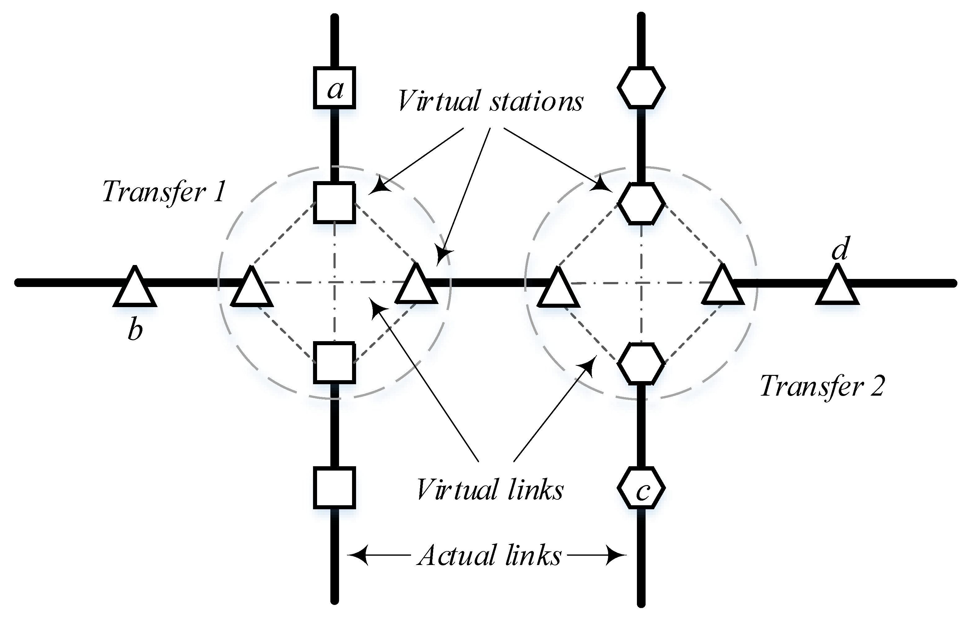
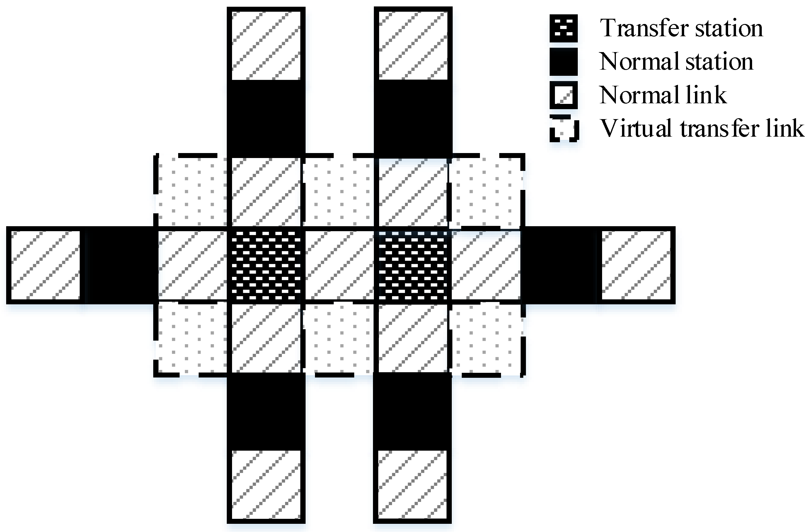
4.1. Augmented Metro Network

Transfer stations in the network connect different metro lines and make it possible for passengers to reach their destinations from origins. Besides the normal function of entrance and exit, passengers’ routing behaviors are more complicated in the transfer stations than in other stations. Especially under metro emergencies, most of the metro passengers have fixed origin and destination, and the commonly used routes on their daily trips. Once they are trapped in a transfer station because of the metro emergencies, they may have to alter their routes to avoid further losses caused by unpleasant delays. However, the interconnected metro network is too complicated, and the sudden change of routes could lead to chaos in transfer stations where passengers with fixed routes may be confused about which route they can choose. As passengers’ destinations could be everywhere, they may switch to all possible directions in the transfer stations.

In order to simplify passengers’ transfer processes, the augmented network [46,47,48,49] is applied in our research, and the structure is shown in Figure 4. The stations draw with short dash lines are virtual stations in the augmented metro network, and the short dash lines between virtual stations are virtual links inside the transfer stations. Virtual links between non-collinear virtual stations inside a transfer station (e.g., short dash lines between virtual triangle station and virtual square station in transfer (1) are the virtual transfer links, representing passengers’ transfer behaviors between different metro lines, and contains transfer attributes like transfer time, transfer distance, etc. Virtual links between two collinear virtual stations (e.g., dot-dash lines between two virtual hexagon stations in transfer (2) are the virtual in-train links contains only metro train dwell time in the transfer station. The solid lines are the actual links in the metro network.

In the augmented metro network, passengers from station a going to station c need to switch twice in transfer 1 and transfer 2, and their route contains 4 virtual stations and 2 virtual transfer links. Route from station b to station c contains 4 virtual stations but only 1 transfer in transfer station 2. Route from station b to station d contains 4 virtual stations and no transfer for station b and d are collinear stations. Travel time on each route is the summation of travel time on actual links, dwell time and transfer time. The number of virtual stations and virtual links is correlated to the number of metro lines that the transfer station connected.

However, when it comes to the real metro network, which the condition is much more complicated. As mentioned above, by the end of 2018, GZM has already possessed over 250 stations. In order to construct the whole Guangzhou metro network with augmented network theory, some basic assumptions are listed below to simplify the unnecessary structures in the network and improve computing efficiency.

(a)

Stations at both ends of a metro line shared with other metro lines as ends are not regarded as transfer stations, for there are fewer transfer passengers in these stations, such as Guangzhou south railway station on line 2 and line 7.

(b)

The metro network is a directed graph, but as the distance and travel time are similar between link l_ij and l_ji, it is regarded as an undirected graph in the simulation and the only difference lies in the directions of the links.

Following these assumptions, we constructed a virtual metro network for GZM. Comparing with the original network, 132 virtual links, and 91 virtual stations are added into the augmented metro network. Totally, the virtual network of Guangzhou metro has 262 stations and 332 links.

4.2. Metro Network with Graph Cellular Automata

CA is a kind of mathematic model that capable of simulating discrete dynamic systems where interactions of the system’s basic elements can lead to global changes in time and space [26]. The main structure of these CA models can be defined as:

$$CA=\left(G,Q,V,f\right)$$

(6)

where the cell space is represented by graph G = (N, L). N(G) is the set of stations {n₁₁, n₁₂, …, n_ij, …, n_nn} in the metro graph G. L(G) is the set of links between different stations, l_ij is the link between station i and station j. N(G) and L(G) are the basic elements in the graph. Q is the states of cells, which is a finite set containing the states of the cells and each cell’s state is related to the state of its u neighbors. V is the neighbor {v₁, v₂, …, v_u} of each cell in the graph where the adjacency matrix can be used to show the connections between each cell. Function f is the cell state transformation function used to describe the changes in cells’ states from time step t to the next time step t + 1. Therefore, the state of station (i, j) in time t + 1 is represented by $Q_{\mathit{ij}}^{t+1}$, which can be described as:

$$Q_{ij}^{t+1}=f\left(Q_{ij}^t,Q_{ab}^t\right)$$

(7)

The states of link l in time t + 1, $Q_{l,\mathit{ij}}^{t+1}$, are determined by the states of the stations they are connected with (i.e., station i and station j). If both of the station i and station j are congested, link l is congested as well. If only one of these two stations is congested, then, the state of link l is either exposed or infected. It is worth noting that one situation is very rare, that is link l is congested while both of the end stations of link l are not congested. In the simulation environment built by the graph-CA, this situation is assumed impossible to appear under metro emergencies.

With the definitions above, the augmented metro network in Figure 4 can be transformed into cell spaces shown in Figure 5.

As a useful generalization and implementation of traditional CA models on graphs, graph-CA provides a method to solve the tough problems of the relationship between structure and process, form and function [33]. Graph-CA’s derivation from both graph theory and CA formalism makes it suitable for the simultaneous use of well-developed ways of describing the model structure and process dynamics. The graph structure enables graph-CA with more flexibility in describing the relationship in a complex system, and the dynamically changing neighborhoods make it capable of reflecting the realistic characteristics in the simulations. In traditional CA, the state of a given cell is defined by the states of cells surround it, that is to say, that the neighborhood relationship is only defined by the positions of the cells. On the contrary, in the augmented network, the neighborhood is defined by both cell positions and their graph relationships (links, arcs, or weights) [38].

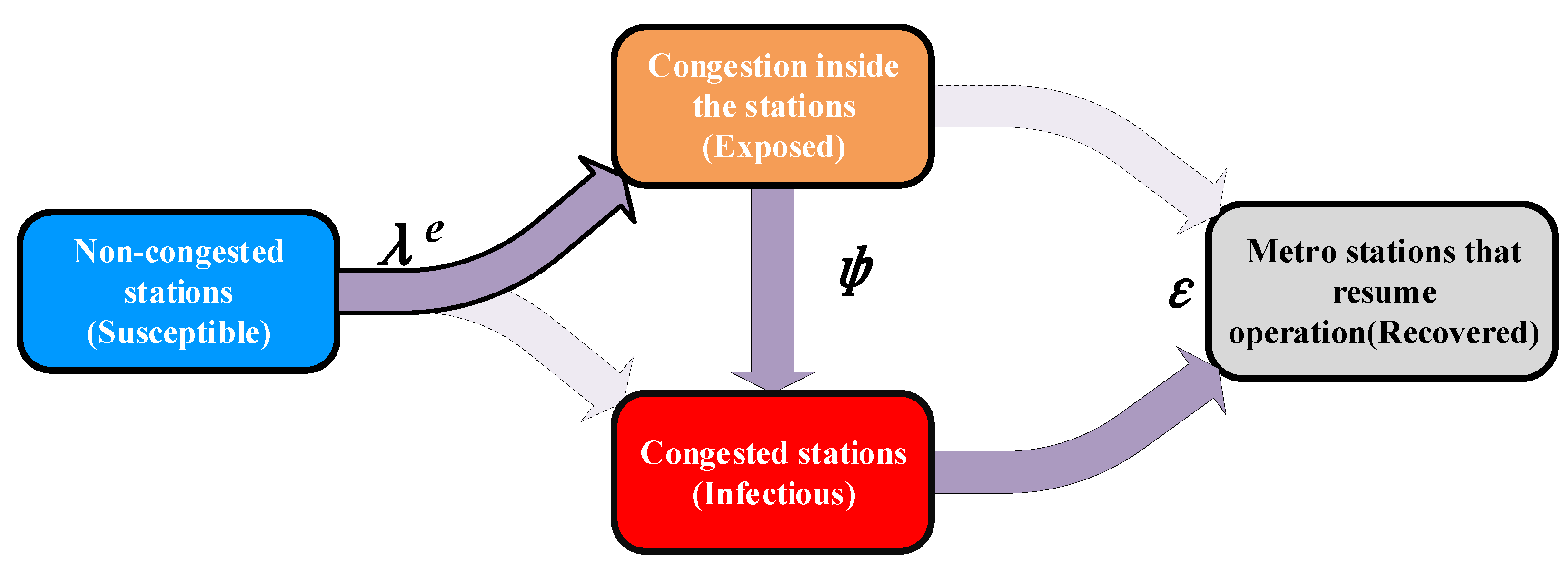
4.3. ASEIR Model with Time Delays

Initially, the traditional SEIR model is used to depict epidemic propagation through complex networks, which contains 4 states: susceptible (S), exposed (E), infectious (I) and recovered (R). Instead of becoming into infectious nodes directly, some susceptible nodes contacted with infectious nodes will become exposed nodes first, before turning into infectious. The exposed nodes need an incubation period to obtain the ability to infect other susceptible nodes, and before the end of its incubation period, the exposed nodes cannot infect nodes connected with them. Therefore, in the SIR model, the congestion is directly transited through the network, whereas the influences of the emergency-caused delays are postponed by the exposed stations in SEIR models.

When the traditional SEIR model is used to simulate travel congestion propagation, the infectious nodes are referred to as the congested to stations or links in the metro network. Once the emergency occurs while metro passengers are traveling inside the metro system, there is another key point to consider that the congestions propagate could be influenced by the network topology. Therefore, in the cell space of the graph-CA environment, the states of station (i, j) in time t of the SEIR model can be defined as $Q_{ij}^t=\left(S_{ij}^t,E_{ij}^t,I_{ij}^t,R_{ij}^t\right)$. Moreover, $S_{\mathit{ij}}^t$ represents the proportion of susceptible metro stations, where susceptible stations are easily transformed into exposed when connected to infectious stations in the metro network. $E_{\mathit{ij}}^t$ is the proportion of exposed (congested) stations, while the exposed stations are unable to spread the congestions to other susceptible stations in the metro network. $I_{\mathit{ij}}^t$ is the proportion of infected stations, and $R_{\mathit{ij}}^t$ is the proportion of recovered stations that have got resistant to the congestions. Since the states of metro stations are all divided into 4 states in the SEIR model, then,

$$S_{\mathit{ij}}^t{+E}_{\mathit{ij}}^t{+I}_{\mathit{ij}}^t{+R}_{\mathit{ij}}^t=1$$

(8)

We have to note that, on one hand, CA models are mathematic methods used to simulate discrete dynamic systems, therefore, in the metro system we investigated, the states of stations are also discrete between time t and time t + ∆t, where ∆t is the time step we used to simulate the congestion propagation in the metro network. In our research, ∆t equals the average section travel time (i.e., the average travel time on a link between two metro stations), which is 2 min averagely in GZM.

On the other hand, the delay-caused incubation time is related to the conditions of each metro station’s properties, where the stations’ various facilities like platforms, staircases, and passageways are distinct from each other. To implement the differences of incubation time in different stations caused by the same metro emergency, we adjusted the traditional SEIR model (i.e., ASEIR model) by assuming the incubation time τ follows gamma distribution, that is, $\mathit{\tau }~\mathsf{\Gamma }(\alpha ,\beta )$, where α is called shape parameter, and β is scale parameter. With a continuous random variable X, and α > 0, β > 0, then, the probability distribution function can be given by Equation (9):

$$f_X\left(x\right)=\{\begin{array}{l}\frac{{\beta }^{\alpha }{x}^{\alpha -1}{e}^{-\beta x}}{\mathsf{\Gamma }\left(\alpha \right)},x>0\\ 0,\mathit{otherwise}\end{array}$$

(9)

where $\mathsf{\Gamma }\left(\alpha \right)$ is the Gamma function, it is a factorial function of positive integers, $\mathsf{\Gamma }(\alpha )=(\alpha -1)!$ However, to any positive number α > 0, $\mathsf{\Gamma }\left(\alpha \right)$ can be calculated using Equation (10):

$$\mathsf{\Gamma }\left(\alpha \right)={\displaystyle {\int }_0^{\infty }{x}^{\alpha -1}{e}^{-x}dx}$$

(10)

Therefore, the ASEIR model with time-postponed τ in the exposed state could be calculated by using Equations (11) to (13).

The fraction of susceptible stations in ASEIR model:

$$S_{ij}^{t+\mathsf{\Delta }t}=S_{ij}^t-{\lambda }^e{S}_{ij}^t{I}_{ij}^t-{\displaystyle \sum _{\left(a,b\right)\in V}\frac{N_{ab}}{N_{ij}}{\lambda }^e{S}_{ij}^t{I}_{ab}^t}$$

(11)

Exposed stations:

$$\begin{array}{l}{E}_{ij}^{t+\mathsf{\Delta }t}=E_{ij}^t+{\lambda }^e{S}_{ij}^t{I}_{ij}^t+{\displaystyle \sum _{\left(a,b\right)\in V}\frac{N_{ab}}{N_{ij}}{\lambda }^e{S}_{ij}^t{I}_{ab}^t}\\ -\left({\lambda }^e{S}_{ij}^{t-\tau }{I}_{ij}^{t-\tau }+{\displaystyle \sum _{\left(a,b\right)\in V}\frac{N_{ab}}{N_{ij}}{\lambda }^e{S}_{ij}^{t-\tau }{I}_{ab}^{t-\tau }}\right)-\phi E_{ij}^t\end{array}$$

(12)

Infectious stations:

$$I_{ij}^{t+\mathsf{\Delta }t}=I_{ij}^t+\left({\lambda }^e{S}_{ij}^{t-\tau }{I}_{ij}^{t-\tau }+{\displaystyle \sum _{\left(a,b\right)\in V}\frac{N_{ab}}{N_{ij}}{\lambda }^e{S}_{ij}^{t-\tau }{I}_{ab}^{t-\tau }}\right)+\phi E_{ij}^t-\epsilon I_{ij}^t$$

(13)

Due to the ridership in the metro network in time t is constant, the total amount of the stations in four states is constant too, so, $S_{ij}^{t+\mathsf{\Delta }t}+E_{ij}^{t+\mathsf{\Delta }t}+I_{ij}^{t+\mathsf{\Delta }t}+R_{ij}^{t+\mathsf{\Delta }t}=S_{ij}^t+E_{ij}^t+I_{ij}^t+R_{ij}^t=1$, and the fractions of recovered stations can be calculated just using Equation (8). λ^e is the congestion propagation rate in the ASEIR model, which changes susceptible stations into exposed stations. N_ab is the ridership transferred from station (a, b) to station (i, j), where station (a, b) is the neighbor stations of station (i, j). N_ij is the total ridership of station (i, j). φ is the transformation rate for station states from exposed to infectious in per time step. ε is the recovery rate of stations changing from infectious to recovered. Unlike epidemic propagation, non-congested (susceptible) stations could transform into congested (infectious) stations directly due to particular conditions, like adjacent stations, particularly crowded space in the stations, and outburst passengers. Figure 6 shows the state transformation process in the ASEIR model in the congestion propagation.

In order to compare the simulation results of the ASEIR model, we also implemented a more commonly used SIR model to simulate the congestion propagation in the metro network. SIR model consists of only three states, susceptible (S), infectious (I) and recovered (R). The propagation process in the SIR model is straight forward, where susceptible nodes will become infectious with a propagation rate once it contacts with infectious nodes in the network. Then, following a certain recover rate, the infectious nodes will become recovered nodes that will be immune to the epidemic forever. SIR model can be defined as $Q_{ij}^t=\left(S_{ij}^t,I_{ij}^t,R_{ij}^t\right)$ in cellular space, and since the stations are consist of these 3 states, then the proportion of each state follows $S_{ij}^t+I_{ij}^t+R_{ij}^t=1$. Moreover, without considering the postponed delays, the station state transformation function of the SIR model can be expressed as Equations (14) to (16).

Fractions of susceptible stations in the SIR model:

$$S_{ij}^{t+\mathsf{\Delta }t}=S_{ij}^t-\lambda S_{ij}^t{I}_{ij}^t-{\displaystyle \sum _{\left(a,b\right)\in V}\frac{N_{ab}}{N_{ij}}\lambda S_{ij}^t{I}_{ab}^t}$$

(14)

Infectious stations:

$$I_{ij}^{t+\mathsf{\Delta }t}=I_{ij}^t-\epsilon I_{ij}^t+\lambda S_{ij}^t{I}_{ij}^t+{\displaystyle \sum _{\left(a,b\right)\in V}\frac{N_{ab}}{N_{ij}}\lambda S_{ij}^t{I}_{ab}^t}$$

(15)

Recovered stations:

$$R_{ij}^{t+\mathsf{\Delta }t}=R_{ij}^t+\epsilon I_{ij}^t$$

(16)

where, $S_{ij}^{t+\mathsf{\Delta }t}+I_{ij}^{t+\mathsf{\Delta }t}+R_{ij}^{t+\mathsf{\Delta }t}=S_{ij}^t+I_{ij}^t+R_{ij}^t=1$, λ is the transformation rate of infectious stations.

It is assumed that five stations on line 8 (Higher education mega center north station, Guanzhou station, Wanshegnwei station, Chebei station and Chebei south station) in Guangzhou metro network are congested because of delays caused by metro emergencies, as shown in Figure 7. These five congested stations are all on the same line, and two of them (Wanshengwei station and Chebei south station) are transfer stations, which could spread the congest condition caused by metro emergencies to the entire metro network.

With the multi-agent-based modeling software package, NetLogo (Center for Connected Learning and Computer-Based Modeling, Northwestern University, Evanston, IL, USA) [50,51], the congestion propagation results on virtual networks of the GZM network are shown in Figure 8. The simulation is carried out with the congestion propagation rate λ = λ^e = 0.7, recovery rate ε = 0.1 and the delay lasts for 10 time steps (20 min). Comparing with the SIR model, the transforming speed from susceptible state to infectious or exposed states in the ASEIR model is much slower, and fewer stations are infected or expose than the SIR model. Moreover, with the effect of delay time, the total number of infected stations in the ASEIR model is larger than the SIR model. Moreover, the infected stations show different tendencies between these two models. At first, the amount of infected stations increases in both models before 60 min (30 time steps, ∆t = 2 min). Then the number of infected stations in the SIR model decreases, but infected stations in the ASEIR model decrease slowly and later (at about 140 min, 70 time steps) reached another peak after the delay is over.

With different congestion propagation rate of 0.5, 0.7 and 0.8 in the ASEIR model, the results of susceptible, exposed, infectious and recovered stations are shown in Figure 9. The double peak property is rather clear in the infected stations under all congestion propagation rates. At the end of the simulation, with a higher congestion propagation rate, more stations remain susceptible and fewer stations become recovered, which indicates that more metro stations are not infected by the congested stations when the transformation rate is high. This is in line with the postponed exposed states that the exposed state is a kind of infected stations but cannot spread congestion to other stations, thus weakened the total effects of the congestion.

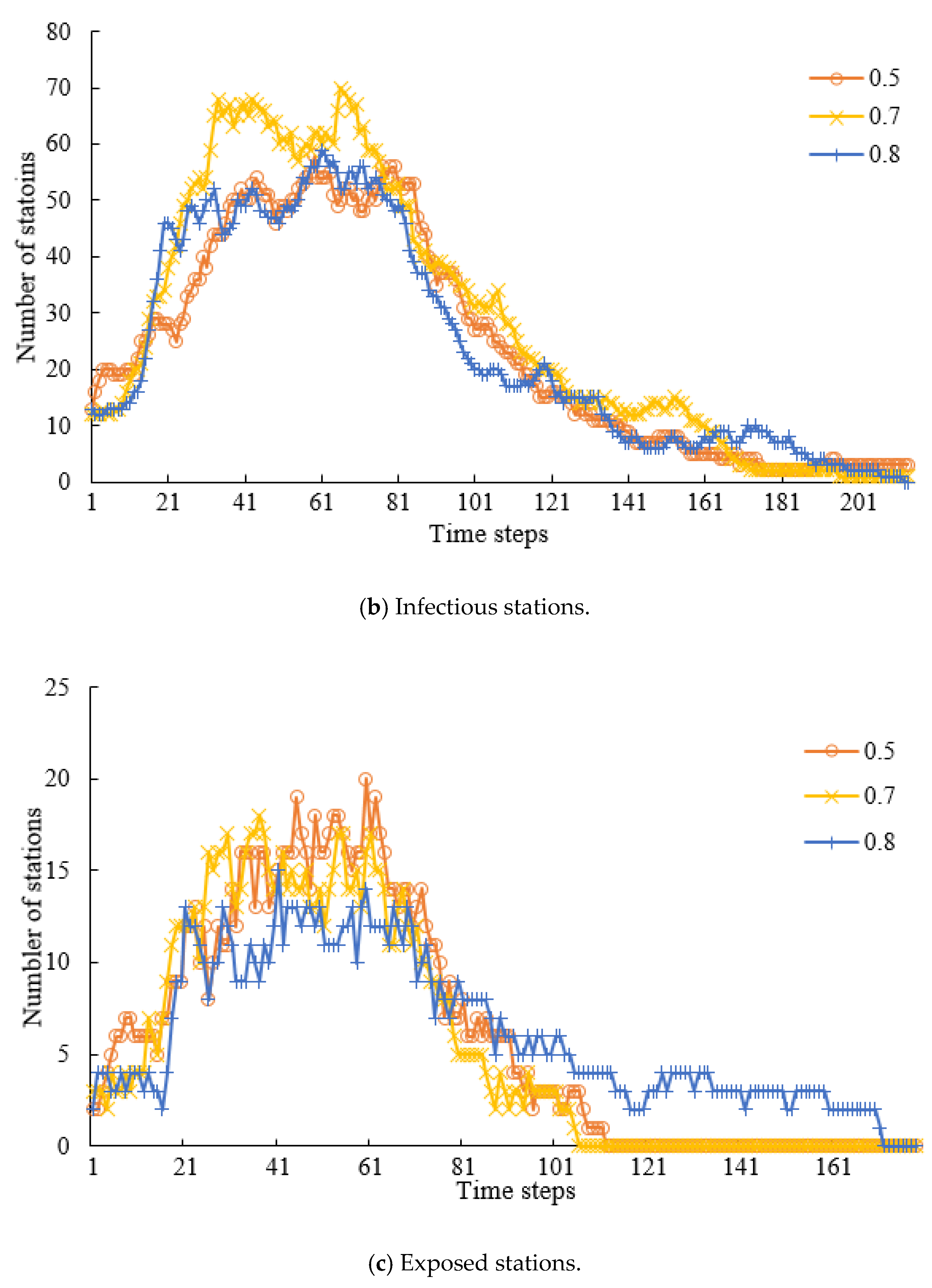
4.4. Quantify Method for Congestion Propagation Rate

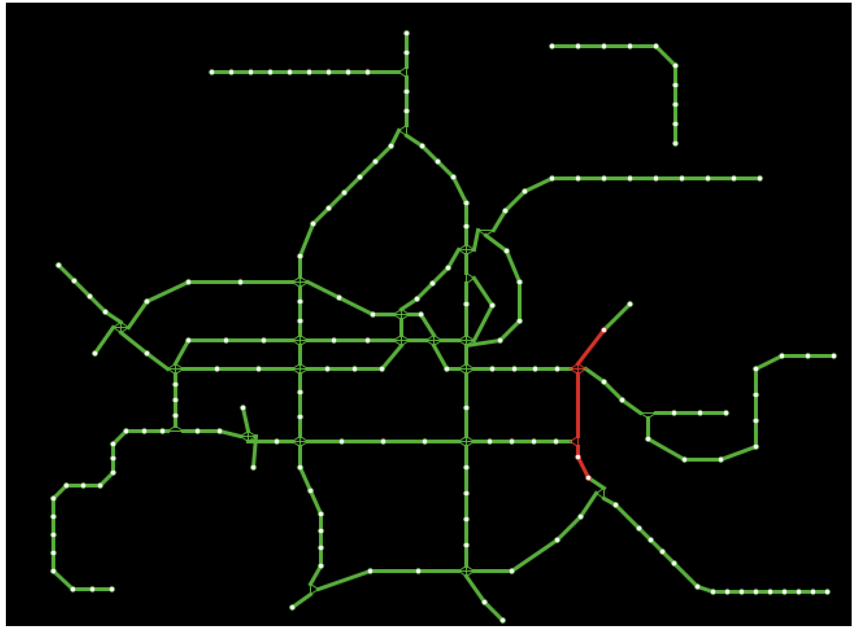
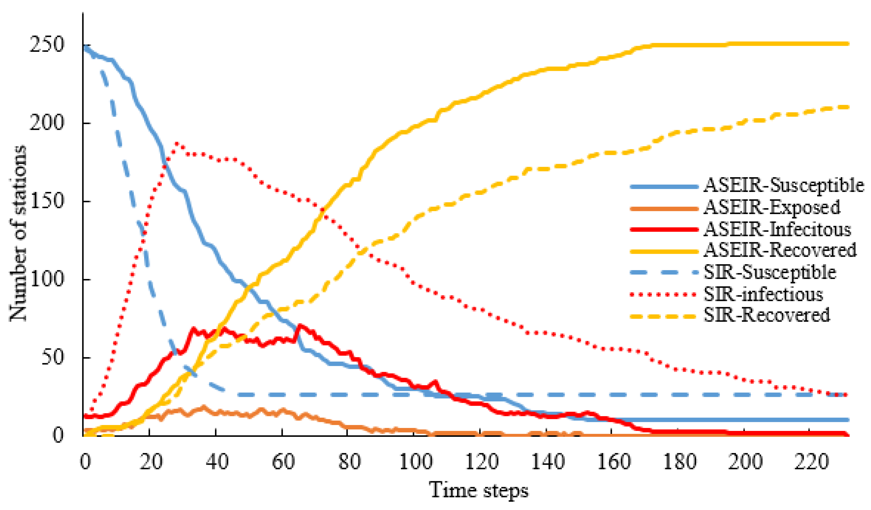
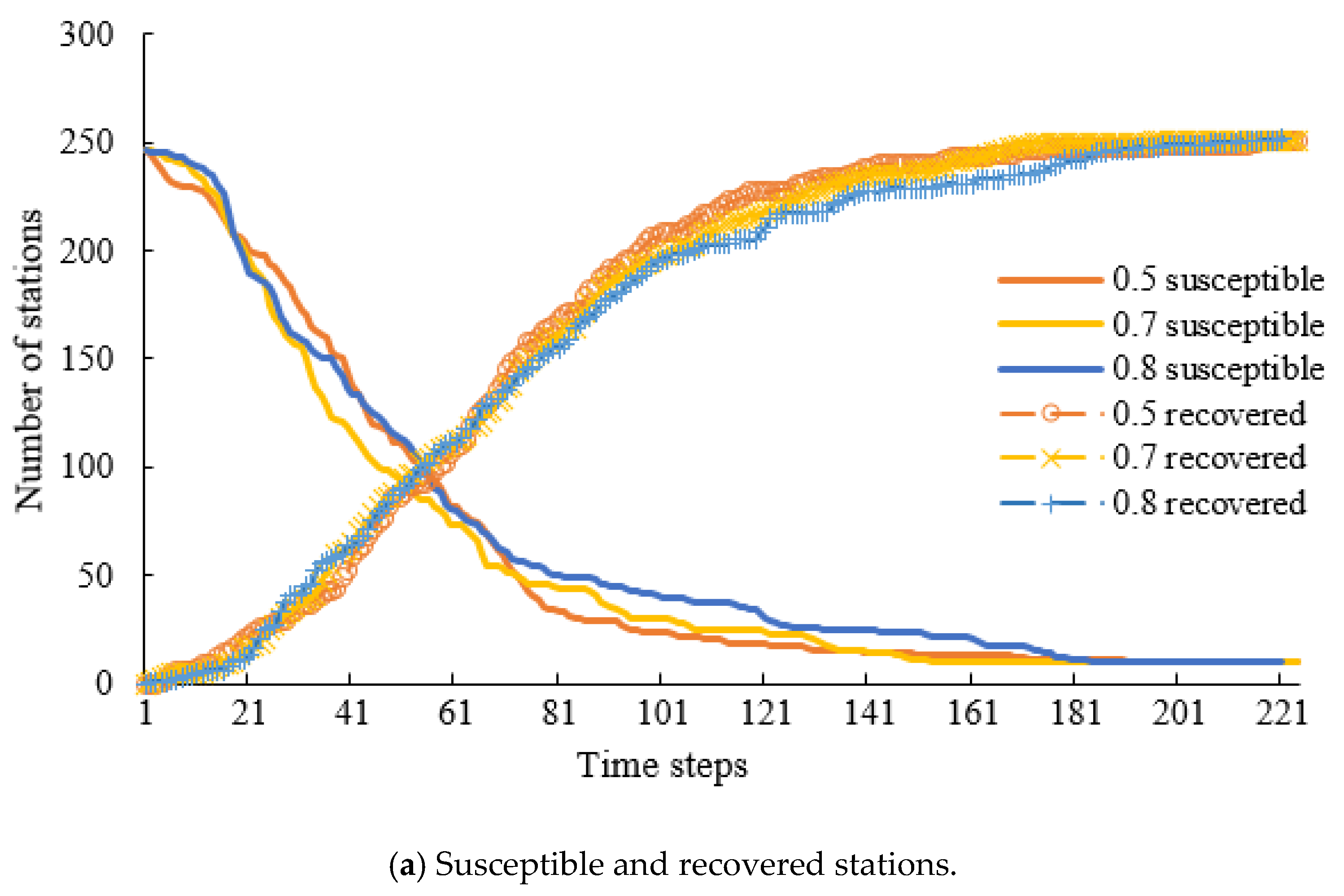
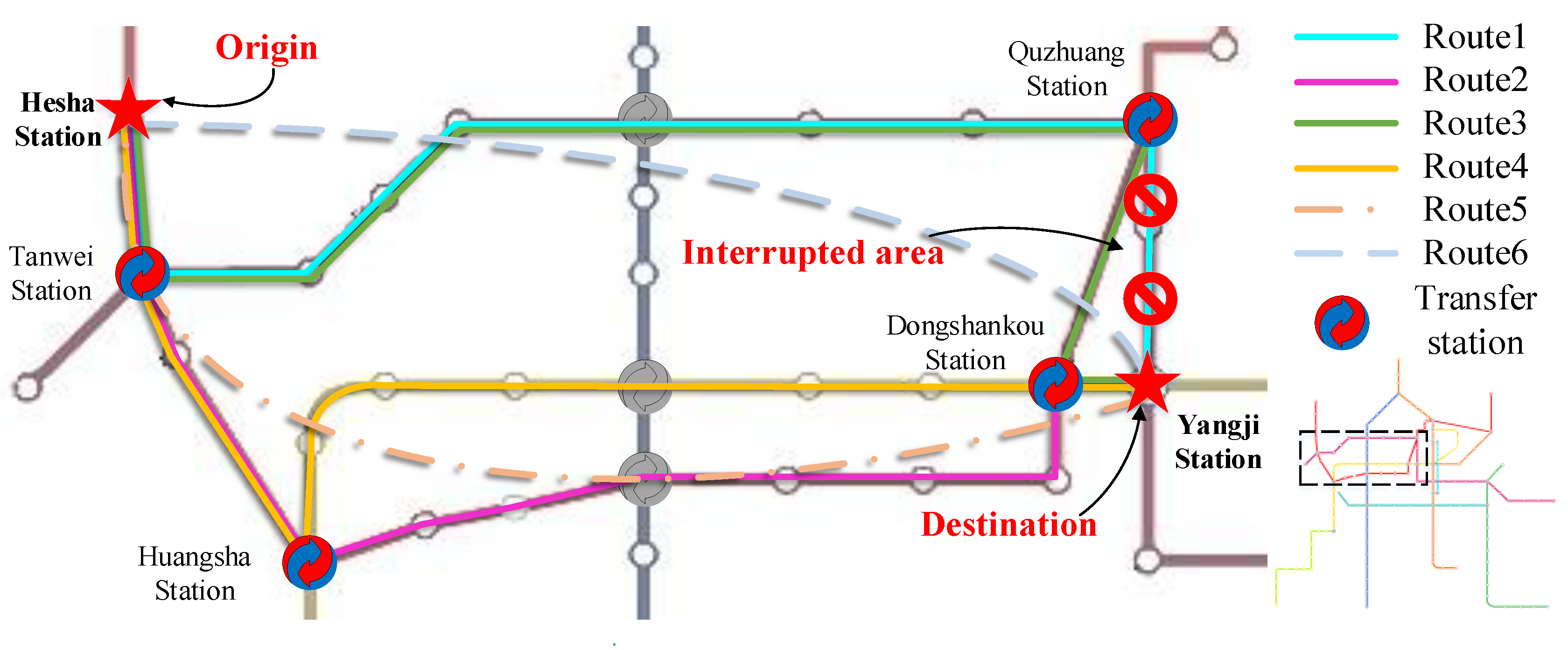
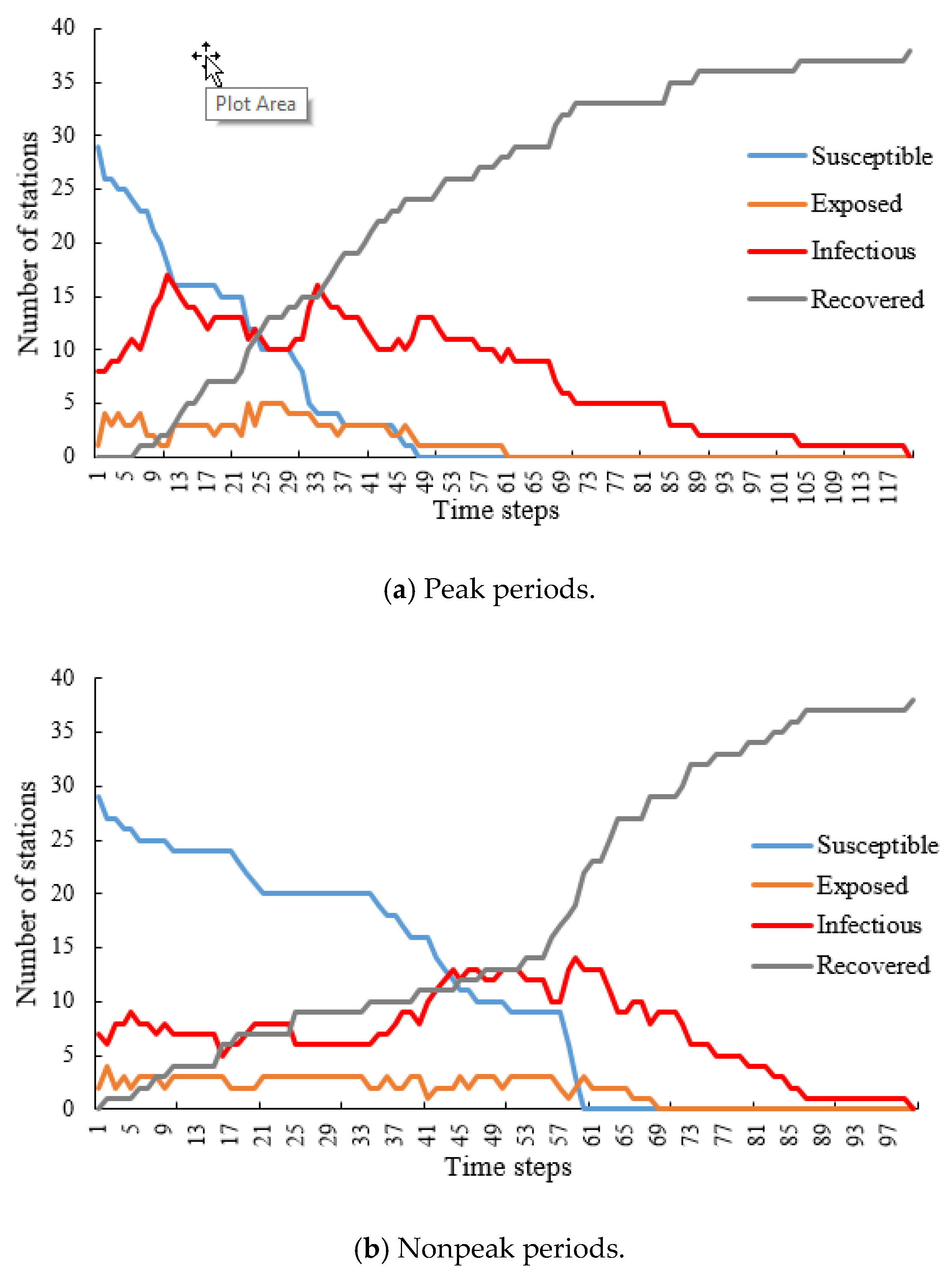
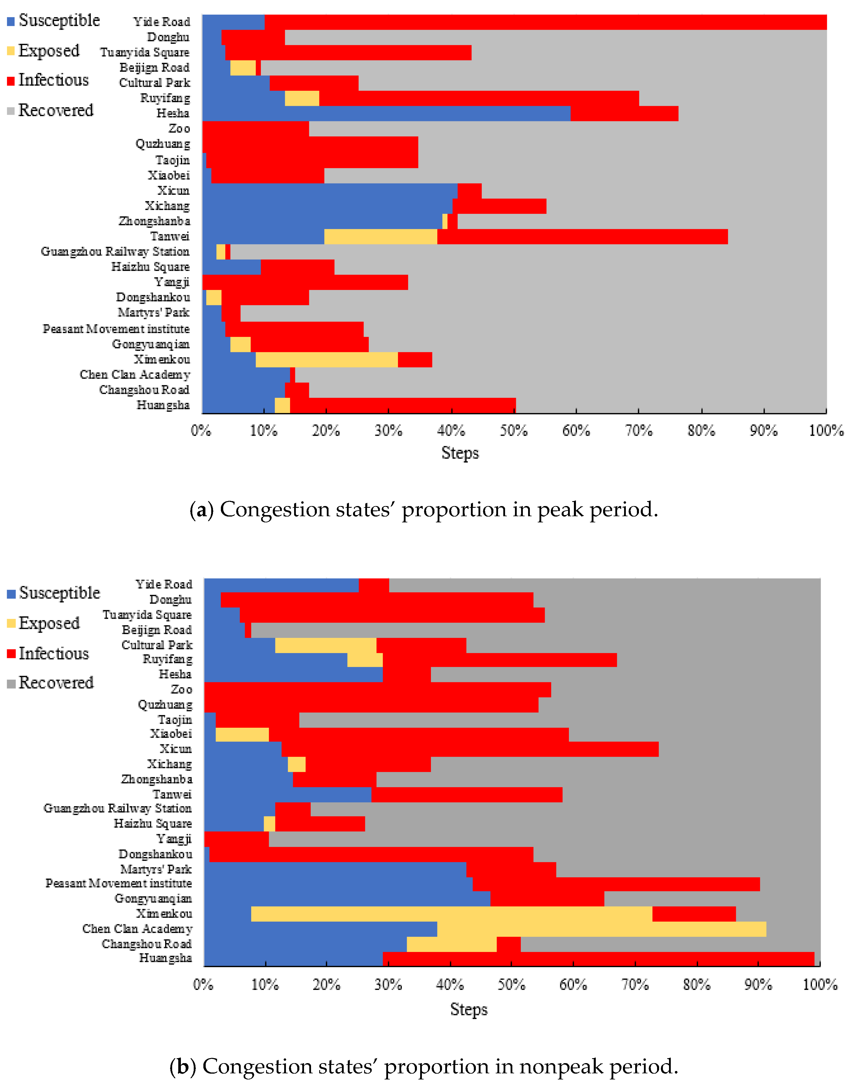
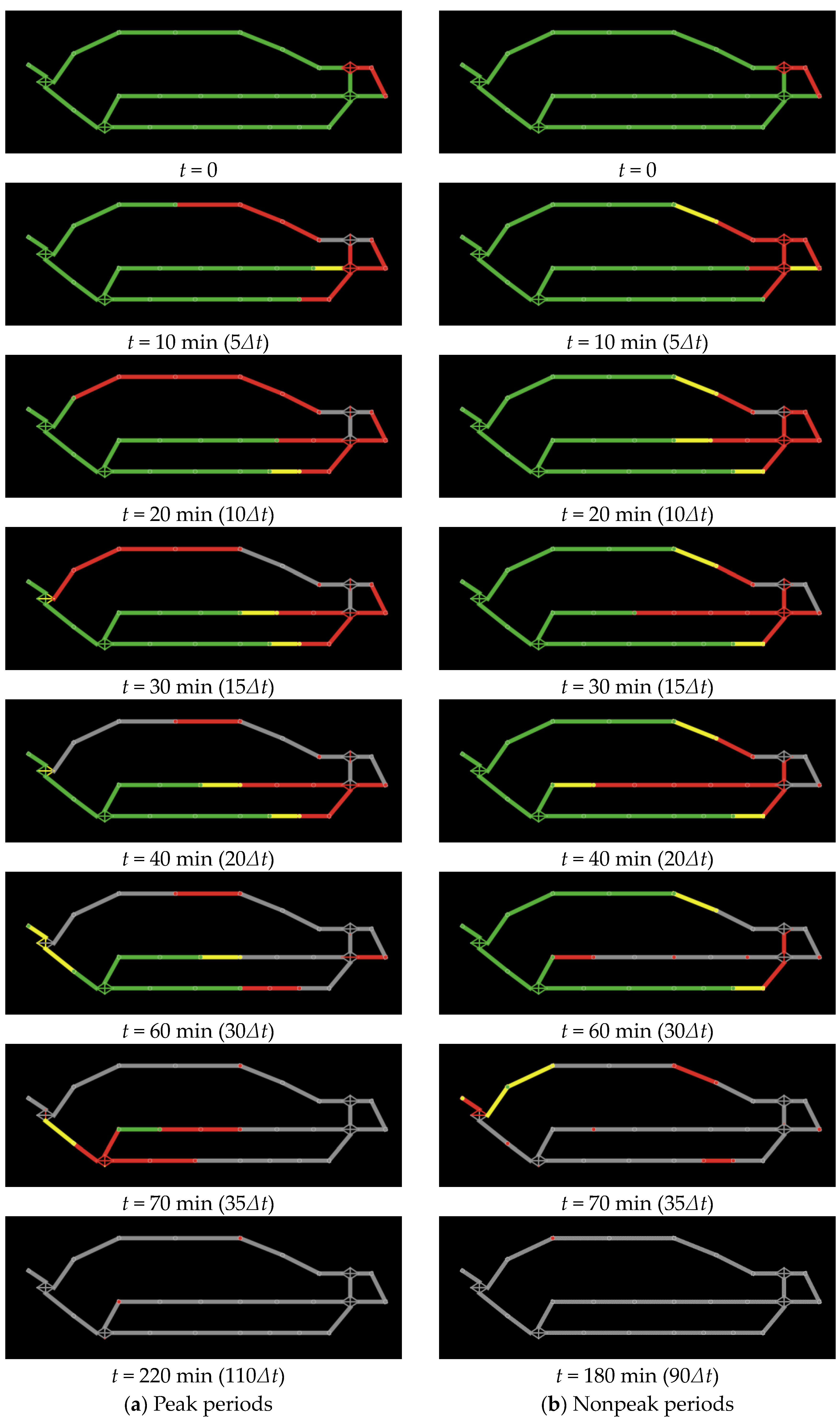
Although the ASEIR model is capable of describing the process of congestion propagation caused by the metro emergencies in the metro network, it is still worth noting that the congestion propagation rate in the aforementioned SIR model and ASEIR model are constant to different stations and ridership situations. It seems unreasonable that the congestion in the metro network spread through different stations at the same speed. Intuitively, stations adjacent to where the metro emergency occurs are more susceptible to the congestions. Meanwhile, they will be the first to become congested stations that further spread the congestion to the entire network. Transfer stations are also vulnerable under this particular condition where the transfers between different lines will be much more frequent than usual. Xiong Z et al. [52] and Zeng Z [53] quantified the metro congestion propagation rate with aggregated ridership data in the framework of the SIR model.

However, another vital element should be taken into account that passengers routing behaviors also have significant influences on the propagation of congestion. Annoyed and may be frustrated by the metro emergencies, the stations on the route that the influenced passengers choose, are the ones that more easily generate congestions alongside the stations on the route. Not to mention that the normally functioning metro lines have already packed with passengers, once encounter the metro emergency influenced passengers, the congestions generate inconvenience to both metro operators and passengers in the crowded underground space.

Therefore, in order to dynamically simulating the congestion propagation process, with the analyzed elements above, the infectious rate ${\lambda }_{ij}^k$ of each station (i, j) on route k can be described by Equation (17)

$${\lambda }_{ij}^k=1-\exp \left[-\left(\frac{H_{ij}^{k,w}}{{\displaystyle \sum _w(H_{ij}^{k,w}+H_{ij}^{w,k})}}\cdot x_1+\frac{C_{ij}^k-V_{ij}^k+O_{ij}-I_{ij}}{C_{ij}^k}+\frac{D{T}_k}{T_k}\cdot x_2+(1-x_2){RSC}_k\right)\right]$$

(17)

where, $H_{\mathit{ij}}^{k,w}$ is the transfer ridership switching route k to route w in transfer station (i, j), on the contrary, $H_{\mathit{ij}}^{w,k}$ is the transfer ridership switch from route w to route k in transfer station (i, j). x₁ is 1 when the station (i, j) is a transfer station, otherwise x₁ equals to 0. $C_{\mathit{ij}}^k$ is maximum transportation capability on the section before station (i, j) on route k. $V_{\mathit{ij}}^k$ is the current section flow on the section before station (i, j) on route k. O_ij and I_ij are outbound ridership and inbound ridership in the station (i, j). x₂ equals 1 when route k is the shortest route of travel time (route l) among all the routes between a certain origin o and destination d, otherwise, x₂ equals 0.

The first term in the exponential terms, the transfer rate, is determined by passengers’ route choices where the influenced passengers could choose to switch their routes to avoid further disturbance of the metro emergency-caused delays. With the estimated parameters in Table 2, the product of route k’s choice probability P(k|C) and the ridership ${\mathit{Rd}}_{\mathit{od}}$ between o and d can be used to represent the ridership on route k, $G_{\mathit{od}}^k$, between origin o and destination d, as shown in Equation (18)

$$G_{od}^k=P(k|C)\cdot R{d}_{od}$$

(18)

Therefore, the transfer ridership can be calculated by Equation (19)

$$H_{ij}^{k,w}=\frac{G_{od}^k}{{\displaystyle \sum _k^{N_{od}}{G}_{od}^k}}$$

(19)

5. Empirical Study

In order to testify the performance of passengers’ routing behavior based congestion propagation rate in the propagation process in the metro network, a small scale of the metro network is selected to reduce the amount of computation and improve operation accuracy. The network we choose is in the central part of Guangzhou metro, as shown in Figure 10, which takes Hesha (HS) station (non-transfer station on Line 6) as the origin station and takes Yangji (YJ) station (transfer station of Line 1 and Line 5) as the destination. The augmented metro network is established, where 38 stations (including 26 actual stations and 12 virtual stations) and 52 links (36 actual links and 16 virtual links) are constructed to reflect passengers travel in the system.

With the k-shortest path algorithm, 4 metro routes are selected to construct the route choice set for the passengers, alongside with 1 bus route and 1 taxi rout. The attributes of the 6 routes are listed in

Table 3. Route attributes from HS to YJ.

Route	AC/m	BC	RSC	Travel Time/min	Transfer Times	Travel Cost/CNY
1	2770.73	0.92	1	23.72	1	5
2	2888.46	0.81	0.43	23.93	1	5
3	3219.03	1.01	0.58	30.88	3	5
4	3020.31	0.79	0.49	26.75	1	5
5	-	-	2.25	63	0	2
6	-	-	0.64	33	0	33

. Where, route 1 is the shortest metro route in travel time (transfer time is included in travel time), route 2 to route 4 are backup routes in the metro system from HS station to YJ station, route 5 travels by bus, route 6 travel by taxi which costs the most among all the routes. Among the metro routes, a total of 26 metro stations are included (about 10% of the stations in the entire metro network), including 4 transfer stations: Tanwei (TW) station, Huangsha (HSha) station, Quzhuang (QZ) station and Dongshankou (DSK) station. There are 3 transfer stations (the gray transfer stations in Figure 10) that do not provide transfer function in this scenario. Therefore, we just regard them as non-transfer stations on the routes.

The interrupted area is placed on route 1 from QZ station to the destination, YJ station, and lead to a delay of about 20 min on route 1, while the other routes are not infected by the metro emergency-caused delay. During the metro delay, passengers can choose all the available routes from route 1 to route 6. Based on the estimated route choice models with the RRM principle in Section 3, the probability of choosing each route is calculated and is shown in

Table 4. Choice probabilities of each route.

Route	M1	M2	M3
1	8.61%	6.75%	10.86%
2	49.83%	48.16%	51.28%
3	34.03%	37.59%	30.13%
4	3.91%	3.41%	4.73%
5	0.89%	0.72%	1.10%
6	2.73%	3.37%	1.91%

. As in line with what we analyzed before, passengers who suffered the metro emergency-caused delays in the peak periods are more likely to abandon the metro and choose taxi as a back option to ensure punctuality. Fewer passengers want to stand still and wait for the resume of the delayed metro line in all periods of the day.

In the ASEIR model, the parameters of M2 and M3 are used, and the simulation results are shown in Figure 11. During peak periods, if there are no intervention measures, it takes 126 time steps (about 4 h) for the network from HS station to HJ station to get rid of the influence of congestion caused by metro emergencies.

In peak periods, the susceptible stations decrease rapidly in the beginning, nearly all the stations are influenced by metro emergency before time step 50. The infectious stations increase quickly and obvious double peaks appear before time step 40, which is consistent with the analysis we made in Section 4. The first maximum value of infectious stations appears at time step 10 (about 20 min), and, coincidentally, the assumption of delay time is 20 min. The variation tendency of exposed stations is in line with infectious stations, which indicates that congestion spread rapidly in the metro network during the time of emergency-caused delays. At about 35 time steps (about 50 min after the first extreme value), as the delay has already ended, the number of exposed stations and infectious stations have another increase and reaches a similar value of the first peak value. Moreover, at time step 49 (less than 2 h), all the stations in the network have been influenced by the congestion, because the amount of susceptible stations has become 0.

During nonpeak periods, the intensity of congestion propagation in the network is obviously moderate comparing with peak periods, and all of the susceptible stations are transferred into exposed stations or infectious stations at time step 60, which is clearly slower than that in peak periods. Moreover, the number of infectious stations reaches its maximum only once, at time step 60, and it is later than peak periods as well. While during nonpeak periods, it only takes about 100 time steps (less than 3 and a half hours), if there are no intervention measures. Therefore, during nonpeak periods, the duration of congestion propagation is also shorter than the duration in peak periods.

In order to investigate the proportions of each state in the entire propagation process, Figure 12 shows the simulation results of all the stations, and each horizontal stripe represents a station’s state. We have to note that as transfer stations contain more than one virtual station, the states of virtual stations determine the state of the transfer station, where the state of infectious is the highest that if one virtual station turns into infectious, then the transfer station is infectious. The priority of the rest states are as follows: exposed > recovered > susceptible. In Figure 12, there are 3 stations (QZ station, Zoo station, and YJ station) congested in the beginning, and these stations in the interrupted area are adjacent to each other.

Due to the high congestion propagation rate during peak periods, the exposed (congested) state in most of the stations are very short, or even in some stations, they just omit the exposed state and immediately transfer into infectious from the susceptible state, such as HS station, Yide Road station, etc. Meanwhile, with more passengers abandon the metro, which diminished the spread of congestion, the duration for stations in the state of congest is shorter than nonpeak periods, as shown in Figure 12b.

The detailed congestion propagation process can be seen in Figure 13, where the green nodes and lines are standing for susceptible stations and links, yellow ones represent exposed stations (and links), the red ones are infectious (congested) and the gray stations and links are in the recovered state.

From the analysis above, we can get a clear picture of the metro congestion propagation process under emergencies. Without intervention measures, congestion caused by emergencies could last for over 3 h in the metro network. During peak hours, congestion spread more intensively both in duration and in scale. Due to a higher transmission intensity, a double peak phenomenon appears in the peak periods. While the congestion propagation during nonpeak periods is much moderate and the congestion only shows one peak in the entire propagation process.

6. Conclusions

In order to get a clear understanding of the dynamical congestion propagation process derived from the metro emergency-caused delays, a simulation model without considering passenger control measures in the entire metro network is investigated. Based on passengers’ spontaneous route choice behaviors under metro emergencies on the microscope level, route choice models based on the RRM principle is develop with passengers’ perceptions on route attributes, network topological factors and delay specific variable. With different route choice models during peak (M2) and nonpeak (M3) periods under metro emergency-caused delays, metro passengers’ heterogeneity is analyzed with SP data collected from GZM passengers. Due to the significant influences of metro emergency-caused delays, passengers behave differently from normal conditions, where they may ignore the normally negative effects of transfers and detour routes to avoid further losses caused by the delays. Moreover, the period when the metro delay occurs is vitally important for its congestion propagation process. Compare with nonpeak periods, a larger proportion of metro passengers travel in peak periods will abandon metro and switch to ground traffic modes like bus and taxi to continue their trip.

Furthermore, a simulation model of congestion propagation using the ASEIR method is proposed in the graph-CA environment with the augmented metro network. In addition, the congestion propagation rate is quantified by integrating passengers’ heterogeneous preferences in route choices under metro emergencies. The simulation result of the ASEIR model considering incubation time reveals the differences in metro emergency-caused delays between peak periods and nonpeak periods. Metro emergency that occurs at peak hours may cause a secondary propagation of congestion in the metro network, while emergencies occur at nonpeak hours has only one peak and has a short duration and smaller influencing range. Therefore, during peak hours, the metro operators not only should take measures to control passenger volumes at the first time when the emergency occurs, but also should pay more attention to the second increase of the congested stations in the secondary congestion propagation process and take targeted measures to reduce the effects of the congestions’ regrowth.

In conclusion, correctly understanding the dynamical congestion propagation process under metro emergencies without intervention measures is the foundation to develop emergency intervention measures and properly control the crowded passenger flow in the metro network. The simulation of metro congestion propagation can provide metro operators a more precise perspective to quantify the influence of the metro emergency-caused delays, and it is a useful method to evaluate the efficiency of the passenger control measures. Additionally, further researches concerning metro passenger control measures and train schedule rearrangements could be tested with the help of these simulation methods, so that the influences and the losses caused by the metro emergencies could be minimized.

References

1. Hu, Y. Study on the Network Characteristics of Urban Rail Transit in Beijing Based on Intelligent Card Data—A Case Study of Beijing; Beijing Jiaotong University: Beijing, China, 2017. [Google Scholar]
2. Wu, Y.; Xu, J.; Jia, L.; Qin, Y. Estimation of emergency evacuation capacity for subway stations. J. Transp. Saf. Secur. 2018, 10, 586–601. [Google Scholar] [CrossRef]
3. Sandeep, M.; Kaan, O.; Bekir, B. Evaluating the resilience and recovery of public transit system using big data: Case study from New Jersey. J. Transp. Saf. Secur. 2018. [Google Scholar] [CrossRef]
4. Chen, W.; Zhang, Y.; Mohammad, K.; Zhao, G. Risk analysis on Beijing metro operation initiated by human factors. J. Transp. Saf. Secur. 2018. [Google Scholar] [CrossRef]
5. Mcfadden, D. The revealed preferences of a government bureaucracy: Theory. Bell. J. Econ. 1975, 6, 401–416. [Google Scholar] [CrossRef]
6. Sheffi, C.F.D. On Stochastic Models of Traffic Assignment. Transp. Sci. 1977, 11, 253–274. [Google Scholar] [Green Version]
7. Heiss, F. Specification(s) of Nested Logit Models; MEA Discussion Paper Series; MEA: New Delhi, India, 2002. [Google Scholar]
8. Yang, Y.; Yao, E.; Yang, Z.; Zhang, R. Modeling the charging and route choice behavior of BEV drivers. Transp. Res. Part C Emerg. Technol. 2016, 65, 190–204. [Google Scholar] [CrossRef]
9. Daniel, M.K.T. Mixed MNL Models for Discrete Response. J. Appl Econ. 2000, 15, 447–470. [Google Scholar]
10. Lee, B.J.; Fujiwara, A.; Zhang, J.; Sugie, Y. Analysis of Mode Choice Behaviors based on Latent Class Models. In Proceedings of the 10th International Conference on Travel Behaviour Research Lucerne, Lucerne, Switzerland, 10–15 August 2003. [Google Scholar]
11. Hess, S.; Stathopoulos, A. Linking response quality to survey engagement: A combined random scale and latent variable approach. J. Choice Model. 2013, 7, 1–12. [Google Scholar] [CrossRef] [Green Version]
12. Sun, Z.; Arentze, T.; Timmermans, H. A heterogeneous latent class model of activity rescheduling, route choice and information acquisition decisions under multiple uncertain events. Transp. Res. Part C Emerg. Technol. 2012, 25, 46–60. [Google Scholar] [CrossRef]
13. Tian, H.; Gao, S.; Fisher, D.L.; Brian, K.P. A Mixed-Logit Latent-Class Model of Strategic Route Choice Behavior with Real-time Information. In Proceedings of the Transportation Research Board Meeting, Washington, DC, USA, 22–26 January 2012. [Google Scholar]
14. Hoogendoorn, S. A State-of-the-Art Review: Developments in Utility Theory, Prospect Theory and Regret Theory to Investigate Travelers’ Behavior in Situations Involving Travel Time Uncertainty. Transp. Rev. 2014, 34, 46–67. [Google Scholar]
15. Chorus, C.G.; Arentze, T.A.; Timmermans, H.J.P. A Random Regret-Minimization model of travel choice. Transp. Res. Part B 2008, 42, 1–18. [Google Scholar] [CrossRef]
16. Chorus, C.G. A new model of random regret minimization. Eur. J. Transp. Infrastruct. Res. 2010, 10, 181–196. [Google Scholar]
17. Charoniti, E.; Rasouli, S.; Timmermans, H.J.P. Context-driven regret-based model of travel behavior under uncertainty: A latent class approach. Transp. Res. Procedia 2017, 24, 89–96. [Google Scholar] [CrossRef]
18. Jing, P.; Zhao, M.; He, M.; Chen, L. Travel Mode and Travel Route Choice Behavior Based on Random Regret Minimization: A Systematic Review. Sustainability 2018, 10, 1185. [Google Scholar] [CrossRef]
19. Thiene, M.; Boeri, M.; Chorus, C.G. Random Regret Minimization: Exploration of a New Choice Model for Environmental and Resource Economics. Environ. Resour. Econ. 2012, 51, 413–429. [Google Scholar] [CrossRef]
20. Kaplan, S.; Prato, C.G. The application of the random regret minimization model to drivers’ choice of crash avoidance maneuvers. Transp. Res. Part F Traffic Psychol. Behav. 2012, 15, 699–709. [Google Scholar] [CrossRef]
21. Hensher, D.A.; Greene, W.H.; Chorus, C.G. Random regret minimization or random utility maximization: An exploratory analysis in the context of automobile fuel choice. J. Adv. Transp. 2013, 47, 667–678. [Google Scholar] [CrossRef]
22. Rasouli, S.; Timmermans, H. Specification of regret-based models of choice behaviour: Formal analyses and experimental design based evidence. Transportation 2016, 44, 1555–1576. [Google Scholar] [CrossRef]
23. Jang, S.; Rasouli, S.; Timmermans, H. Incorporating psycho-physical mapping into random regret choice models: Model specifications and empirical performance assessments. Transportation 2016, 44, 999–1019. [Google Scholar] [CrossRef]
24. Toffoli, T.; Margolus, N.H. Invertible Cellular Automata: A Review; Cellular Automata; MIT Press: Cambridge, MA, USA, 1990; Volume 45, pp. 229–253. [Google Scholar]
25. Santé, I.; García, A.M.; Miranda, D.; Crecente, R. Cellular automata models for the simulation of real-world urban processes: A review and analysis. Landsc. Urban Plan. 2010, 96, 1–122. [Google Scholar] [CrossRef]
26. Li, K.; Gao, Z.; Ning, B. Cellular automaton model for railway traffic. J. Comput. Phys. 2005, 209, 179–192. [Google Scholar] [CrossRef]
27. Zheng, Y.; Xi, X.; Zhuang, Y.; Zhang, Y. Dynamic Parameters Cellular Automaton Model for Passengers in Subway. Tsinghua Sci. Technol. Int. J. Inf. Sci. 2015, 20, 594–601. [Google Scholar] [CrossRef]
28. Stevens, D.; Dragicevic, S. A GIS-based irregular cellular automata model of land-use change. Environ. Plan. B Plan. Des. 2007, 34, 708–724. [Google Scholar] [CrossRef]
29. Dahal, K.R.; Chow, T.E. Characterization of neighborhood sensitivity of an irregular cellular automata model of urban growth. Int. J. Geogr. Inf. Syst. 2015, 29, 475–497. [Google Scholar] [CrossRef]
30. Shi, W.; Pang, M.Y.C. Development of Voronoi-based cellular automata -an integrated dynamic model for Geographical Information Systems. Int. J. Geogr. Inf. Syst. 2000, 14, 455–474. [Google Scholar] [CrossRef]
31. White, R.; Engelen, G. Cellular automata and fractal urban form: A cellular modelling approach to the evolution of urban land-use patterns. Environ. Plan. A 1993, 25, 1175–1199. [Google Scholar] [CrossRef]
32. Osullivan, D. Graph-Cellular Automata: A Generalised Discrete Urban and Regional Model. Environ. Plan. B Plan. Des. 2001, 28, 687–705. [Google Scholar] [CrossRef] [Green Version]
33. Martinez, M.J.; Merino, E.G.; Sanchez, E.G.; Sánchez, J.E.G.; del Rey, A.M.; Sánchez, G.R. A graph cellular automata model to study the spreading of an infectious disease. In Proceedings of the Mexican International Conference on Artificial Intelligence, San Luis Potosi, Mexico, 27 October–4 November 2012; pp. 458–468. [Google Scholar]
34. Rin, P.R.; Dalp, D.D.; Ven, M.J.; Clausse, A. Graph-based Cellular Automata for Simulation of Surface Flows in Large Plains. Asian J. Appl. Sci. 2012, 5, 224–231. [Google Scholar] [Green Version]
35. Krzysztof, M.; Jarosław, J.; Rokita, M. Application of Graph Cellular Automata in Social Network Based Recommender System. In Proceedings of the International Conference on Computational Collective Intelligence, Craiova, Romania, 11–13 September 2013. [Google Scholar]
36. Tretyakova, A.; Seredynski, F.; Bouvry, P. Cellular Automata Approach to Maximum Lifetime Coverage Problem in Wireless Sensor Networks. Simul. Trans. Soc. Model. Simul. Int. 2014, 92, 153–164. [Google Scholar]
37. Małecki, K. Graph Cellular Automata with Relation-Based Neighborhoods of Cells for Complex Systems Modelling: A Case of Traffic Simulation. Symmetry 2017, 9, 322. [Google Scholar] [CrossRef]
38. Bodo, A.; Katona, G.Y.; Simon, P.L. SIS Epidemic Propagation on Hypergraphs. Bull. Math. Biol. 2016, 78, 713–735. [Google Scholar] [CrossRef] [Green Version]
39. Liu, J.; Zhang, T. Epidemic spreading of an SEIRS model in scale-free networks. Commun. Nonlinear Sci. Numer. Simul. 2011, 16, 3375–3384. [Google Scholar] [CrossRef]
40. Raveau, S.; Guo, Z.; Munoz, J.C.; Wilson, N.H.M. A behavioural comparison of route choice on metro networks: Time, transfers, crowding, topology and socio-demographics. Transp. Res. Part A Policy Pract. 2014, 66, 185–195. [Google Scholar] [CrossRef]
41. Raveau, S.; Munoz, J.C.; De Grange, L. A topological route choice model for metro. Transp. Res. Part A Policy Pract. 2011, 45, 138–147. [Google Scholar] [CrossRef]
42. Zhang, Y.; Yao, E.; Dai, H. Transfer volume forecasting method for the metro in networking conditions. J. China Railw. Soc. 2013, 35, 1–6. [Google Scholar]
43. Newman, M. Networks: An Introduction. Astron. Nachr. 2010, 327, 741–743. [Google Scholar]
44. Daniel, S.; Yuhan, Z.; Qing-Chang, L. Vulnerability Analysis of Urban Rail Transit Networks: A Case Study of Shanghai, China. Sustainability 2015, 7, 6919–6936. [Google Scholar] [Green Version]
45. Mcfadden, D. Quantitative Methods for Analyzing Travel Behaviour of Individuals: Some Recent Developments; Cowles Foundation Discussion Papers; Yale University: New Haven, CT, USA, 1978. [Google Scholar]
46. Si, B.; Zhong, M.; Sun, H.; Gao, Z. Equilibrium model and algorithm of urban transit assignment based on augmented network. Sci. China Technol. Sci. 2009, 52, 3158–3167. [Google Scholar] [CrossRef]
47. Wu, J.; Sun, H.; Gao, Z.; Han, L.; Si, B. Risk-based stochastic equilibrium assignment model in augmented urban railway network. J. Adv. Transp. 2014, 48, 332–347. [Google Scholar]
48. Si, B.; Zhong, M.; Yang, X.; Gao, Z. Urban transit assignment model based on augmented network with in-vehicle congestion and transfer congestion. J. Syst. Sci. Syst. Eng. 2011, 20, 155–172. [Google Scholar] [CrossRef]
49. Zhang, Y.; Yao, E.; Zhang, J.; Zhang, K. Estimating metro passengers’ path choices by combining self-reported revealed preference and smart card data. Transp. Res. Part C Emerg. Technol. 2018, 92, 76–89. [Google Scholar] [CrossRef]
50. Wilensky, U. Center for Connected Learning and Computer-Based Modeling. In NetLogo; Northwestern University: Evanston, IL, USA, 1999; Available online: http://ccl.northwestern.edu/netlogo/ (accessed on 7 January 2019).
51. Wilensky, U. NetLogo 6.1.0. User Manual. Available online: http://ccl.northwestern.edu/netlogo/docs/ (accessed on 13 May 2019).
52. Xiong, Z.H.; Yao, S.Z. Congestion Propagation Quantization Model about Rail Transit System. J. Transp. Syst. Eng. Inf. Technol. 2018, 18, 146–151. [Google Scholar]
53. Zeng, Z. Analyzing Congestion Propagation on Urban Rail Transit Oversaturated Conditions: A Framework Based on SIR Epidemic Model. Urban Rail Transit 2018, 4, 130–140. [Google Scholar] [CrossRef]
Figure 1. Delay information sent out by PIDS in the GZM network.
Applsci 09 04210 g001
Figure 2. Respondents attribute in the SP survey.
Applsci 09 04210 g002
Figure 3. Passengers’ endurance of delay time in different period.
Applsci 09 04210 g003
Figure 4. Structure of augmented metro network.
Applsci 09 04210 g004
Figure 5. The augmented metro network in graph-CA.
Applsci 09 04210 g005
Figure 6. Congestion propagation process in the metro network using the ASEIR model.
Applsci 09 04210 g006
Figure 7. Congestion in GZM network.
Applsci 09 04210 g007
Figure 8. Simulation results of the SIR model and the ASEIR model.
Applsci 09 04210 g008
Figure 9. Stations’ states in ASEIR simulation.
Applsci 09 04210 g009aApplsci 09 04210 g009b
Figure 10. Available routes from HS station to YJ station.
Applsci 09 04210 g010
Figure 11. Congestion propagation during peak and nonpeak periods.
Applsci 09 04210 g011
Figure 12. Congestion states in the GZM network.
Applsci 09 04210 g012
Figure 13. Congestion propagation process in GZM.
Applsci 09 04210 g013