Fault Data Detection of Traffic Detector Based on Wavelet Packet in the Residual Subspace Associated with PCA

Abstract

To improve the accuracy and efficiency of fault data identification of traffic detectors is crucial in order to decrease the probability of unexpected failures of the intelligent transportation system (ITS). Since convolutional fault data recognition based on traffic flow three-parameter law has a poor capability for multiscale of fault data, PCA (principal component analysis) is adopted for traffic fault data identification. This paper proposes the fault data detection models based on the PCA model, MSPCA (multiscale principal component analysis) model and improved MSPCA model, respectively. In order to improve the recognition rate of traffic detectors’ fault data, the improved MSPCA model combines the wavelet packet energy analysis and PCA to achieve traffic detector data fault identification. On the basis of traditional MSPCA, wavelet packet multi-scale decomposition is used to get detailed information, and principal component analysis models are established on different scale matrices, and fault data are separated by wavelet packet energy difference. Through case analysis, the feasibility verification of traffic flow data identification method is carried out. The results show that the improved method proposed in this paper is effective for identifying traffic fault data.

1. Introduction

With the development of sensors, computers and communication technologies, more and more high-speed and high-precision sensors are applied in the field of traffic detection. As a result, the amount of data in traffic database is also growing rapidly [1]. At the same time, due to the inconsistency of the front-end sensors and the changeability of the natural environment, the traffic data obtained contains not only normal traffic information, but also abnormal data caused by electromagnetic interference, detector failure, transmission network failure and traffic accidents—thus affecting the reliability of the intelligent transportation system (ITS) [2]. Therefore, it is of great practical significance to carry out research on the fault data diagnosis technology of traffic detectors to effectively improve the reliability of ITS operations [3].

After combing through the previous work in detail, the methods of data process monitoring can divided into three categories: mathematical model-based, knowledge-based and data-driven methods. In the urban traffic system, the data acquired by the detector is huge and the system dynamics are complex. It is impossible to establish an accurate mathematical model for such a system. Moreover, the knowledge or experience of experts is also subjective. However, the monitoring process data contains abundant process information, and the operation status of the system can be characterized by the normal or abnormal data. It is pointed out in the literature [4] that research is gradually changing from a model-based approach to a data-driven approach. Literature [5] divides data-driven monitoring methods into machine learning, signal processing, and multivariate statistics. Machine learning methods aim at the correct rate of fault diagnosis [6]. They train machine learning algorithms such as neural networks [7] or support vector machines [8] to diagnose faults by using historical data of objects in normal and various fault situations. It has a wide range of applications, but, because of the need for sample data in case of process faults, and the accuracy of the algorithm being closely related to the completeness and representativeness of the samples, it is difficult to be used in those processes that can not obtain a large amount of fault data. Signal processing methods use signal processing methods such as spectral analysis and wavelet transform to analyze the time-frequency characteristics of measured signals, and then diagnose faults [9]. The multivariate statistical analysis method is represented by principal component analysis (PCA). PCA is the core of data-driven process control and fault diagnosis [10]. It constructs a new set of latent variables and forms a new mapping space based on the original data space. The main change information is extracted from it and the statistical features are extracted, so that the spatial characteristics of the original data can be tabulated and the spatial dimension of the original data can be reduced. At the same time, the projection space statistical eigenvectors are orthogonal to each other, which eliminates the correlation between variables and greatly reduces the complexity of the original process characteristic analysis.

Given their importance, the fault data detection of traffic detectors is always a research focus and has attracted the attention of numerous scholars for years [11]. At present, the research of traffic detector fault data recognition mainly focuses on data fault identification based on a traffic flow three-parameter rule [12], data fault identification based on statistical analysis and data fault identification based on artificial intelligence [13]. Xu [14], by analyzing the influence of inner relationship of data acquisition interval and three traffic flow parameters, then designed a four-step data sieving method. In the literature [15], for the non-stationary traffic flow data, wavelet analysis is used to separate the high-frequency and low-frequency components of the original traffic flow data, and then the least squares method is used to find the abnormal points in the reconstructed signal data, which effectively reduces the false positive rate and the false negative rate. Ngan [16] presents a Dirichlet process mixture model (DPMM) for detecting abnormal data in large-scale traffic data, and the experimental results show that the method has good robustness. In literature [17,18], a clustering method is proposed to detect hardware data errors and abnormal traffic behavior in collected large-scale traffic data. The abnormal values are detected by the relationship between neighborhoods of data points, and the ST (space-time) signal of traffic video is transformed into a two-dimensional vector by principal component analysis (PCA). When applied to data fault detection, PCA is only applicable to the analysis of fault samples that exist on a single scale or frequency segment [19,20,21]. However, the fault data often occur in different time-frequency ranges in the actually collected sample data. That is, the sample data are multi-scale in nature, so the traditional PCA cannot be applied to diagnose the fault data in this situation [22]. For this reason, Bakshi [22] first proposed a multi-scale principal component analysis (MSPCA) model, and the basic principle of MSPCA is to combine wavelet and principal component analysis, extend the single-scale model to a multi-scale model, combine the ability of principal component analysis to reduce the dimension linearly with the ability of removing the autocorrelation of process variables by wavelet and the advantage of decisive feature of process variables by wavelet. Then, the wavelet coefficients are analyzed by PCA on various scales. In the study of traffic detector data, it is found that normal traffic data are regular and its signal energy range is relatively fixed. When abnormal data appear in the data, it will be directly reflected in the signal energy of the collected data. This anomaly may be caused by noise and may also be a traffic detector failure. Therefore, this article only detects where there is an exception in the detected data, and does not calculate the size of the exception.

Aiming at the problem of fault in dynamic traffic data, the fault data detection models based on PCA model, MSPCA model and improved MSPCA model were proposed respectively in this paper. First, the wavelet packet is used to decompose the original data with multi-scale, and the individual variable was decomposed into approximation coefficients and detail coefficients of multiple scales and the corresponding principal component analysis models in various scale matrices were established. Then, using the model statistical magnitude as the threshold value, the comprehensive principal component analysis model was obtained by reconstructing wavelet coefficients and the fault data were separated.

The innovative contributions of this paper can be summarized as follows:

(1)

Aiming at the fault problem of dynamic traffic data, a fault data detection model based on principal component analysis (PCA) is proposed. The principal component subspace and residual subspace are established by historical data. The obtained traffic detector data are projected into the space, and the data to be checked are described by parameters.

(2)

In order to solve the problem of fixed MSPCA modeling and single problem with principal component subspace and $T^2$, SPE parameters. Using the idea of adaptive PCA principal component recursion for reference, the wavelet decomposition is replaced by the wavelet packet decomposition, and the fault data are detected by the energy difference of the wavelet packet, which improves the resolution of the model.

The structure of this paper is as follows: Section 2 briefly introduces the fundamental theories of wavelet packet energy analysis and the principal component analysis theory. The third section, the core idea and detailed process of the fault data recognition model are expounded. The fourth section tests the fault data recognition model based on the actual detector data and validates its effectiveness; Section 5 concludes the paper.

2. Preliminaries

In this section, firstly, the basic theory of wavelet packet is elaborated. Then, the basic theory of principal component analysis is elaborated.

2.1. The Basic Theory of Wavelet Packet Energy Analysis

In the process of data failure identification, the fault data are realized by calculating the energy difference between the wavelet packet component of normal data and the corresponding component containing the fault data. Some of the fault information is sometimes hidden in high frequency information and cannot be found in wavelet decomposition. The difference between wavelet packet decomposition and wavelet is that the former decomposes the wavelet decomposition into the same low-frequency part of the same layer in the high-frequency part of each layer. Therefore, in the fault diagnosis process, the wavelet packet algorithm is more suitable than the wavelet decomposition algorithm.

In the Mallat algorithm, there are impulse response functions $h\left(n\right)$ and $g\left(n\right)$. Therefore, the scale function $\phi \left(t\right)$ and the wavelet function $\psi \left(t\right)$ are defined as follows [23]:

$$\left\{\begin{array}{c}\phi \left(t\right)={\sum }_{n}h\left(n\right)\phi (2t-n),\hfill \\ \psi \left(t\right)={\sum }_{n}g\left(n\right)\psi (2t-n).\hfill \end{array}\right.$$

(1)

In Formula (1), $g\left(n\right)={(-1)}^{1-n}h(1-n)$, n is the wavelet packet decomposition channel number. Set a finite energy signal, using the Formula (1), the scale function and the wavelet function can be obtained, and the wavelet packet decomposition is obtained as follows [24]:

$$\left\{\begin{array}{cc}{u}_{2j}\left(t\right)=\sqrt{2}{\sum }_{k\in Z}h\left(k\right)u_j(2t-k),\hfill & \\ u_{2j+1}\left(t\right)=\sqrt{2}{\sum }_{k\in Z}g\left(k\right)u_j(2t-k),\hfill & \hfill 1\le j\le J,\\ u_0\left(t\right)=x\left(t\right).\hfill & \end{array}\right.$$

(2)

In Formula (2), $u_j\left(t\right)$ is a wavelet packet coefficient, and j is the decomposition scale, $k\in Z,k\ge 2$, means the scale factor k is an integer not less than 2, $h\left(k\right)$ is the low pass filter coefficient, $g\left(k\right)$ is the high pass filter coefficient, $x\left(t\right)$ is a finite energy signal.

Wavelet packet energy formula is defined as:

$$E={\int }_{-\infty }^{+\infty }{x}^2\left(t\right)dt=\sum _{a=1}^{2^j}\sum _{b=1}^{2^{j-1}}{\int }_{-\infty }^{+\infty }{x}_j^a\left(t\right)x_j^b\left(t\right)dt=\sum _{n=0}^{2^j-1}{E}_j^n.$$

(3)

In the form: $x\left(t\right)$ is a finite energy signal, scale parameter j, scale factor a and displacement factor b of basis function $\psi \left(t\right)$. $E_j^n={\int }_{-\infty }^{+\infty }{x}_j^i{\left(t\right)}^{2}dt$, and is the data energy of the n-th band in the j-th scale decomposition of the decomposed signal. Thus, the wavelet packet energy difference is as follows: $\Delta E_j^n=E_j^n-E_j^{n\left(d\right)}$, $E_j^n$ is the normal data of wavelet packet energy, and $E_j^{n\left(d\right)}$ is the data to be seized wavelet packet energy.

In any interval, when a fault occurs, the energy difference in the fault point and its vicinity will be abruptly changed, and the energy difference between the data points without fault occurring will be relatively gentle. Therefore, the wavelet packet energy difference is sensitive to the fault data, which can be used to analyze and identify the fault on multiple scales.

2.2. Principal Component Analysis Theory

A traffic detector has many characteristics, such as a large number of sensors, a large dimension of data collected, and a large amount of data. Taking the coil sensor as an example, a section contains only two intersections. If we need to collect enough abundant data, we need several or even more coils, which makes it possible to obtain a large amount of data in a sampling period. Principal component analysis ($PCA$) is a branch of multivariate statistics, which is especially suitable for multivariate data processing [25].

Principal Component Analysis ($PCA$) is one of the projection models in multivariate statistical analysis. The principle is to assume that there is a measurement sample containing m sensors: $x\in R^m$. In the measurement sample, each sensor has n independent sampling data, and the data are constructed into a data matrix of size $m\times n$:

$$X={[x_1,x_2,\dots ,x_n]}^T\in R^{n\times m}.$$

(4)

Each column of X represents a measurement variable, and each row represents a sample. The PCA model first standardizes each sample of X, that is, it calculates the covariance matrix of X, and the formula is as follows:

$$cov\left(x\right)\approx \frac{X^T·X}{n-1}.$$

(5)

After the feature decomposition of X is completed, the size of the feature values is sorted from large to small. The $PCA$ model decomposes X as follows:

$$\left\{\begin{array}{c}X=\widehat{X}+E=T·P^T+E,\hfill \\ T=X·P.\hfill \end{array}\right.$$

(6)

After separating the fault data, the variable with a larger contribution graph is considered as the cause variable that may generate fault data.

In Equation (6), $P\in$R${}^{m\times A}$ is the load matrix and is composed of the first A feature vectors of $cov\left(x\right)$. $T\in$R${}^{n\times A}$ is a score matrix, each column of T is called a principal element variable, A is the number of principal elements, and is also the number of columns of the score matrix. It can be known from the properties of the eigenvalues and the eigenvectors that the scoring matrices are mutually orthogonal, so these principal elements are also independent of each other. The covariance of the principal element can be calculated from Equation (7):

$$\Lambda =\frac{X^T·X}{n-1}=\left[\begin{array}{cc}{\lambda }_1& \\ \dots & \dots \\ & {\lambda }_n\end{array}\right],$$

(7)

where ${\lambda }_1\ge {\lambda }_2\ge \dots .\ge {\lambda }_n$ represents the top A larger eigenvalues of covariance matrix of X. For the selection of principal A, this paper uses the method of calculating the cumulative variance contribution rate to determine. 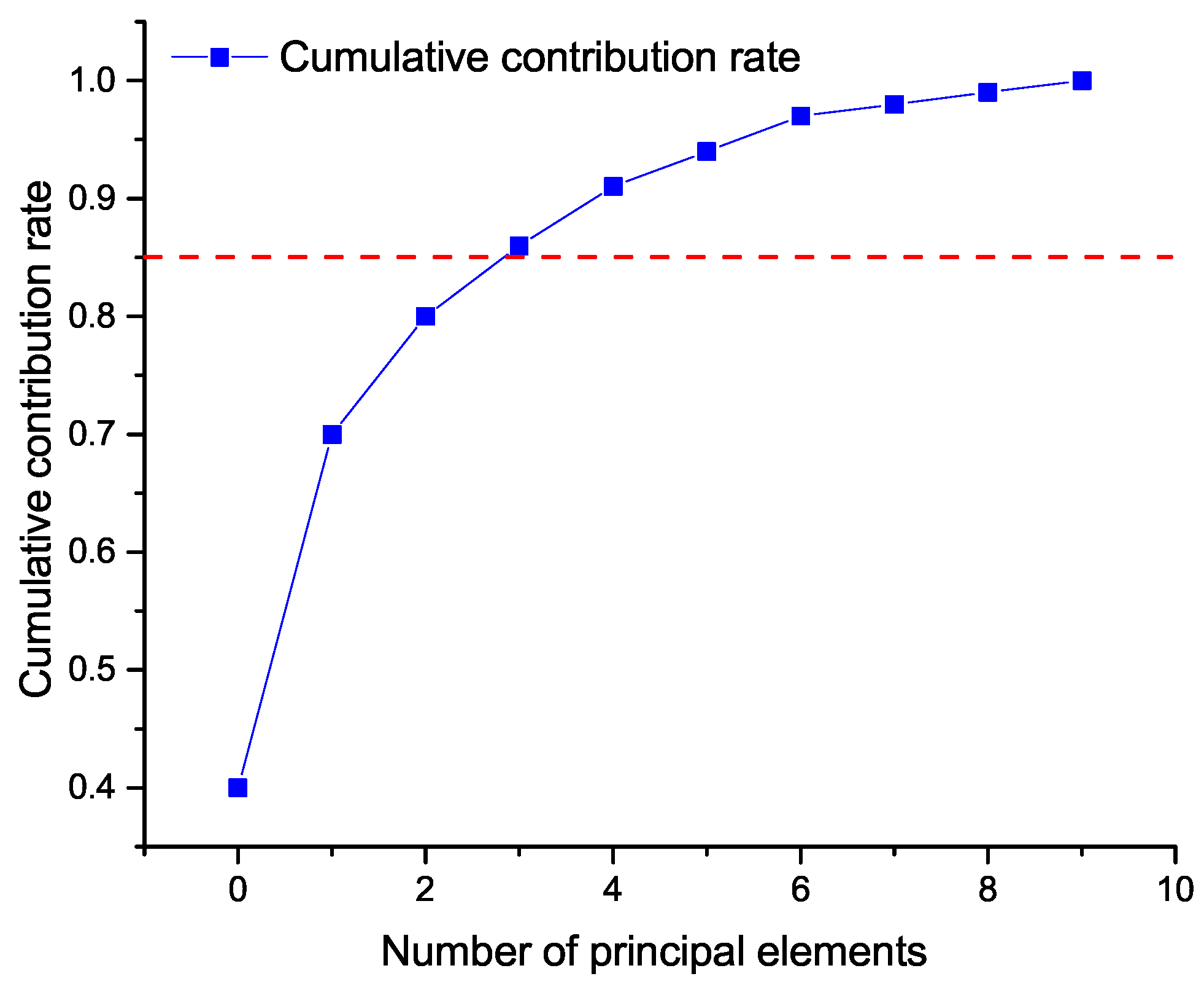The cumulative variance contribution rate represents the ratio of the amount of data that the first A principals can interpret to the total data [26]. This can be calculated as follows:

$$CPV=\frac{{\displaystyle \sum _{i=1}^A}{\lambda }_i}{{\displaystyle \sum _{i=1}^m}{\lambda }_i}.$$

(8)

Usually, when the CPV (cumulative contribution percentage of variance) reaches more than 85%, it can be assumed that the former A principal component can explain most of the data changes in X. As shown in Figure 1, the red dashed line represents the value of CPV, which is 85% in Figure 1, when the lower limit of CPV is set at 85%, the number of principals is at least two. Therefore, when three principals are selected, the first three principals can contain enough information.

The principal component constitutes a space, which is called the principal subspace, and the orthogonal complementary space is called the residual subspace. Any sample vector in X can be decomposed into projections on principal and residual subspaces [26].

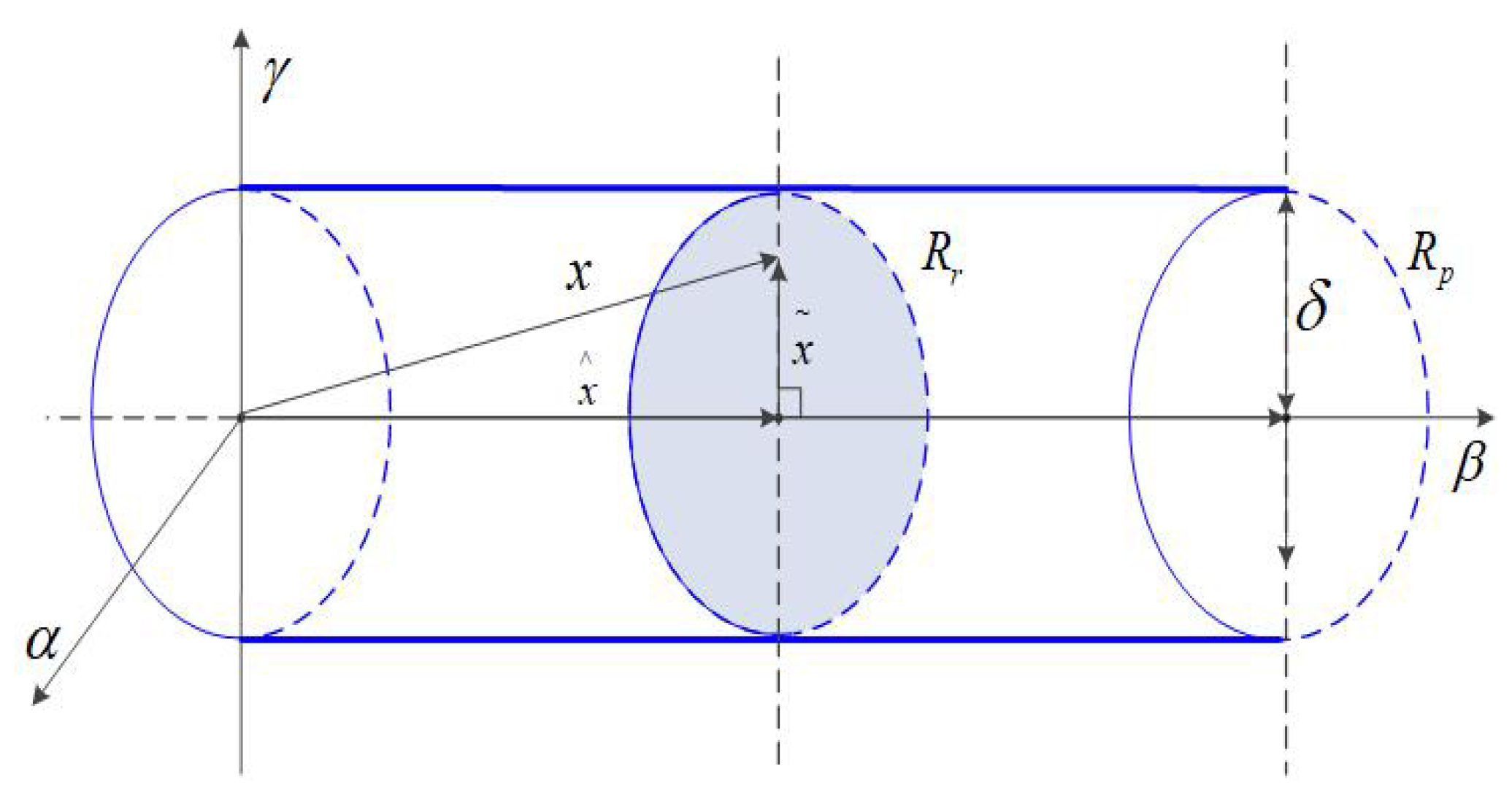
As shown in Figure 2, X is the measurement data matrix, x is the measurement sample, $\beta$ is the principal subspace direction, and $\alpha$ and $\gamma$ are the residual subspace directions. X is projected in two directions to form two spaces, namely principal subspace $R_p$ and residual subspace $R_r$. The projection result in the $R_p$ direction is $\widehat{x}$, that is, the size of the effective data component in the sample. $\tilde{x}$ is a projection on the residual subspace.

The PCA model divides the variable space into two orthogonal and mutually exclusive subspaces. Any sample vector can be decomposed into projections on these two spaces: $x=\tilde{x}+\widehat{x};$ $\widehat{x}=P{P}^{T}x\in R_p;$ $\tilde{x}=(I-P{P}^T)x\in R_r$. $\widehat{x}$ is the modeled part and $\tilde{x}$ is the unmodeled part. From the above relationship, we can conclude that: $(I-P{P}^T)·\widehat{x}=0,(I-P{P}^T)·\tilde{x}=0$. Because it is orthogonal projection, the two satisfy the orthogonal relationship: ${\widehat{x}}^T\tilde{x}=0$. In addition, the two are not statistically relevant, so there are:

$$E\left(\widehat{x}{\tilde{x}}^T\right)\approx \frac{X^{T}X}{n-1}=\frac{P{T}^T\overline{X}}{n-1}=0.$$

(9)

From the above analysis, we can find that PCA has natural advantages in process monitoring. It is very suitable for real-time monitoring of traffic detector data.

3. Proposed Fault Diagnosis Method

In this section, the fault data detection models based on the PCA model, MSPCA model and improved MSPCA model are introduced, respectively.

3.1. Diagnostic Model Based on Principal Component Analysis

Based on PCA, the idea of fault separation is to build two spatial models through a large number of normal offline data, and then detect the detected data, separate the correct data and fault data separately. In measuring the normal data, we usually use the Squared prediction error $\left(SPE\right)$ and Hotelling’s $T^2$ (hereinafter referred to as statistics $T^2$) to identify whether there is an abnormality [27].

The $SPE$ indicator measures the variation of the sample vector in the residual space projection:

$$SPE={∥(I-P{P}^T)x∥}^2\le {\delta }_{\alpha }^2.$$

(10)

In Formula (10), ${\delta }_{\alpha }^2$ represents the control limit when the confidence level is $\alpha$, the calculation formula is as follows: ${\delta }_{\alpha }^2=g{\chi }_{h;\alpha }^2$, $g=\frac{{\theta }_2}{{\theta }_1}$, $h=\frac{{\theta }_1^2}{{\theta }_2}$, $h_0=1-2\frac{{\theta }_1{\theta }_3}{3{\theta }_1^2}$, ${\theta }_i={\displaystyle \sum _{j=A+1}^m}{\lambda }_j^i(i=1,2,3)$.

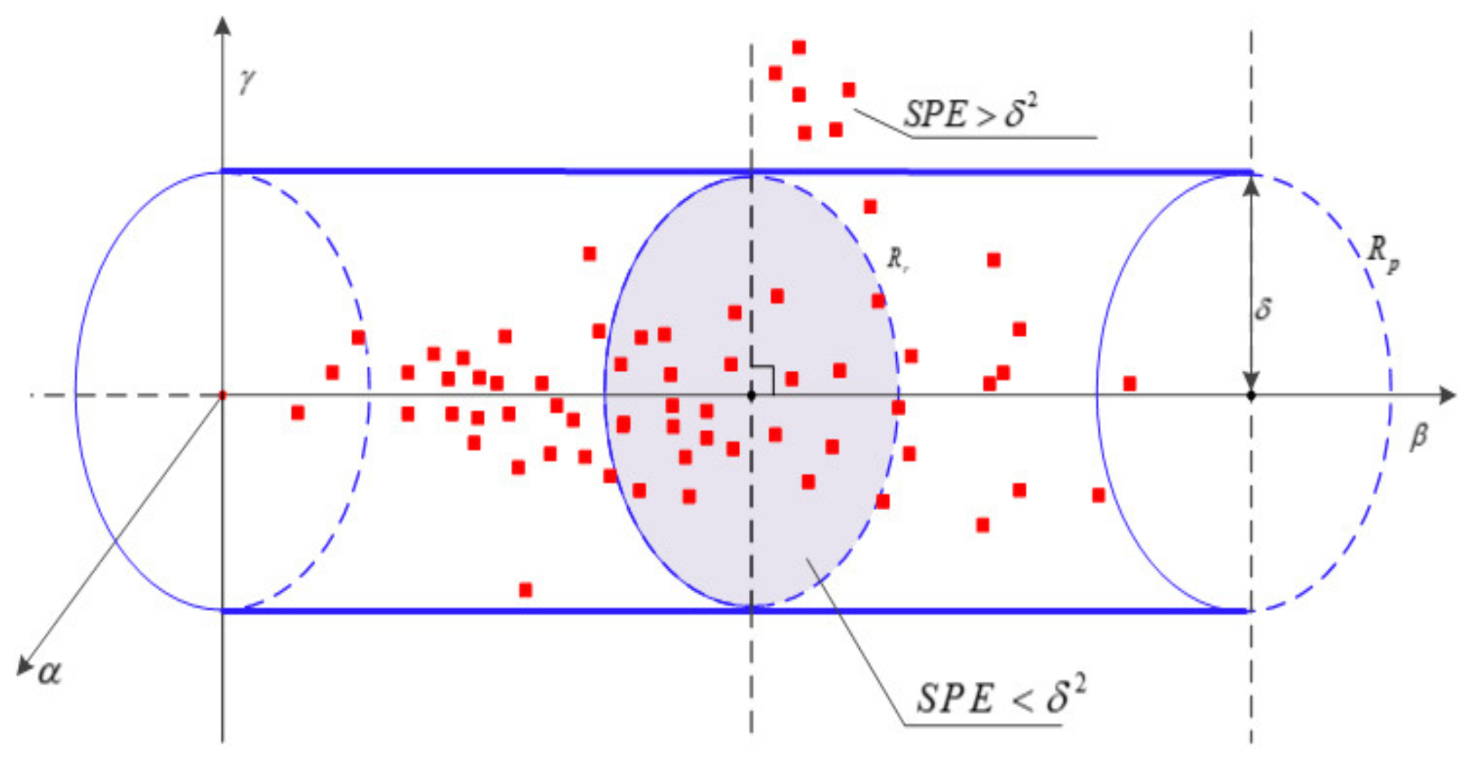
${\chi }_{h;\alpha }$ is the distribution critical value of degree of freedom h and confidence $\alpha$. The occurrence of faults is reflected in the statistical index exceeding the statistical control limit, and the change of correlation between data are reflected in the change of SPE value. Fault detection based on SPE is shown in Figure 3. $\delta$ is the radius of control domain, the red dot represents the data point, and the distance from the data point to the $\beta$-axis is SPE of residual space. If this distance is maintained in a controllable domain, it indicates that no fault occurs, and, if the data point falls outside the domain, it is considered that a fault occurs.

$T^2$ statistics measure the change of variables in the principal element space:

$$T^2=x^{T}P{\Lambda }^{-1}{P}^{T}x\le T_{\alpha }^2.$$

(11)

In Formula (11), $\Lambda =diag\left\{{\lambda }_1,\dots ,{\lambda }_A\right\}$, $T_{\alpha }^2$ represents the $T^2$ control limit when the confidence degree is $\alpha$.

Although both SPE and $T^2$ indicators are used for process fault detection, it is important to point out that the two indicators are complementary. The SPE indicator measures the degree of correlation change between normal process variables and shows abnormal process conditions. The $T^2$ indicator measures the distance of an existing sample from the origin of the principal subspace. Since the principal subspace contains most of the change in the signal when the process is normal, and the residual subspace mainly represents noise, the control limit defined by $T^2$ is usually much larger than that defined by SPE [28]. Therefore, smaller faults easily exceed the control limits of the SPE. If the $T^2$ indicator of a sample exceeds the control limit, its SPE indicator does not exceed its control limit, that is, it does not destroy the relationship between variables. This situation may be a fault, or the process scope may change.

After the completion of the fault data detection, the need to separate the variable that caused the fault. In the process of fault diagnosis of a traffic detector, it is most likely to find out which sensor occurs when the data anomaly is found. The fault separation method used in this paper is a fault separation method based on the SPE contribution graph. The calculation method is as follows [28]:

$$SPE={∥\tilde{C}x∥}^2=\sum _{i=1}^{m}Con{t}_i^{SPE}.$$

(12)

In Formula (12), $Con{t}_i^{SPE}={\left({\zeta }_i^T\tilde{C}x\right)}^2$, $Con{t}_i^{SPE}$ represents the contribution value of each variable to the statistic $SPE$ for the data matrix X to be picked up. $\tilde{C}=I-P{P}^T$, ${\zeta }_i$ represents the $i-th$ column of the identity matrix $I_m$. Figure 3 shows the geometric schematic of fault detection based on SPE index. After the fault is separated, the variable with a larger contribution graph is considered to be the cause variable that may cause the fault.

3.2. Fault Data Recognition Model Based on MSPCA

In the long-term study and summary of traffic detectors, it is found that, due to the aging of sensors in detectors and the wear and tear of various devices, traffic flow parameters detected during a certain period of time seem to be at a normal level with little fluctuation of data, but the offset of data are more and more significant, along with this kind of gradual cumulative failure. Ultimately, it will cause systematic false alarm and is not easy to detect.

With the maturity of wavelet technology, the multi-scale characteristics of fault data have made remarkable progress. In order to provide more detailed and high-resolution analysis data and to overcome the shortcomings of customer service PCA, Bakshi [22] proposed a multi-scale principal component analysis fault diagnosis method. This model does not depend on the analytical model of the target system, but proceeds from the process data, combines wavelet analysis with PCA, and uses PCA to process more offline data. The multiscale characteristic of wavelet is used to overcome the shortcomings of conventional PCA in meta-statistical analysis.

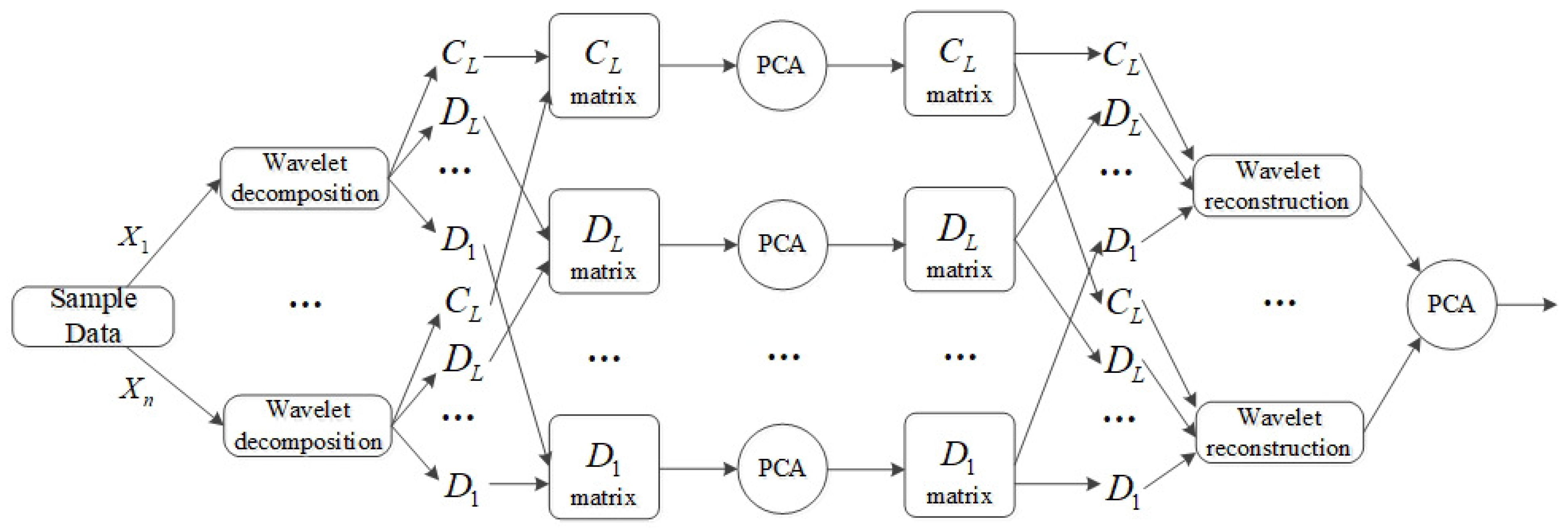
Figure 4 is the flow chart of MSPCA. It can be seen from the graph that MSPCA combines wavelet analysis with PCA organically. The model uses offline normal data to establish principal component subspace, then decomposes the sample data by wavelet, and models the coefficient matrix of wavelet analysis coefficients separately in principal component space. After reconstructing the decomposed signal, the principal component will be modeled again.

3.3. Fault Data Recognition Model Based on Improved MSPCA

When monitoring the actual dynamic traffic data, the noise distribution of the data are random and its intensity is time-varying. However, when dealing with the wavelet coefficients beyond the control threshold, the traditional MSPCA uses the unified threshold under the decomposition scale to reconstruct the wavelet, lacking the consideration of the time-varying noise. Therefore, part of the noise will be mistaken as fault data and separated into residual space. In addition, part of the fault data covered by noise will be expanded, resulting in an increased false alarm rate.

In order to solve the problems of a fixed model, principal component subspace, SPE, $T^2$ and a single parameter in traditional MSPCA, based on the recursive idea of the adaptive PCA, the traditional MSPCA is adjusted. The modifications are as follows:

(i)

Segmental processing of collected traffic flow data;

(ii)

In order to improve the resolution of the model, the wavelet decomposition is adjusted to the wavelet packet decomposition;

(iii)

The energy difference of nodes in each decomposition scale is calculated by the energy difference of wavelet packet to locate the fault data location.

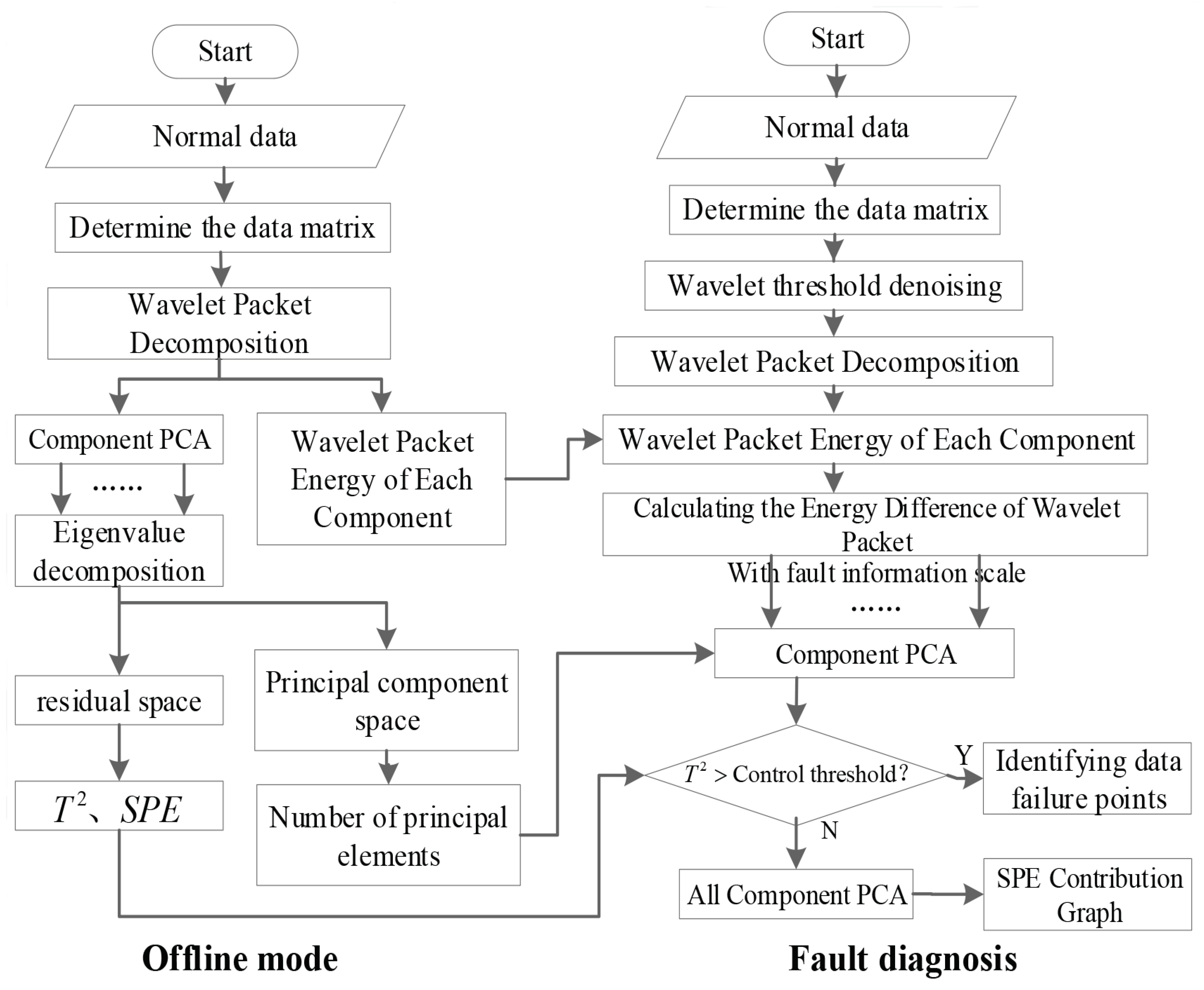
Figure 5 shows the flow chart of the improved method.

The model is mainly divided into two modules: offline module and online fault diagnosis module. The offline module preprocesses the model with normal data. Through this process, the scale parameters of wavelet packet and the number of principal components of principal component analysis can be determined. The online fault detection module uses the parameters calculated by the offline module to monitor the online data in real time, remove the noise interference, and finally complete the data fault diagnosis.

As shown in Figure 5, in offline mode, the model firstly preprocesses the normal historical data, uses the wavelet packet to decompose the data at $J-level$, calculates the wavelet packet energy of each component on each scale, and models the component data on each scale by PCA, and chooses the appropriate number of principal components. The data space is decomposed into principal component space and residual space, and the control limits of $T^2-SPE$ statistics for each component on each scale are calculated.

In the online fault diagnosis mode, the data are denoised by wavelet threshold. Referring to the scale parameters calculated in the offline mode, the data are decomposed into J-scales. The wavelet packet energy of each component on the scale is calculated, and the difference of wavelet packet energy on each scale is obtained. According to the set threshold, the fault can be judged. The components with faults are selected for principal component analysis, and the location and size of data faults are determined according to $T^2-SPE$ control limits obtained from offline mode. Finally, all the data are analyzed by PCA to determine which sensors are responsible for the fault and the severity of the fault.

The detailed algorithm process is as follows:

Step1

Input the normal data matrix X, set the size of the data window is m, and N is a multivariate variable dimension;

Step2

The wavelet packet transform is used to decompose each row of the data matrix X, that is, each variable to a scale J, and to calculate the wavelet packet energy value of each component under the scale;

Step3

Perform the principal component analysis on each wavelet packet component to calculate the number of each principal component and the two control-limit parameters of the component;

Step4

Input the online monitoring data, carry out the wavelet threshold diagnosing for each component, and reconstruct the wavelet packet with the same scale according to the corresponding components in Step2;

Step5

Calculate the wavelet packet energy of each component. In addition, subtract from the corresponding offline data wavelet packet energy, to obtain the components of the wavelet packet energy difference curve;

Step6

Select the faulty component or the component of interest, and perform the principal component modeling of the same parameters as in Step3, and use the previously obtained SPE control parameter and control parameter to separate the fault;

Step7

Repeat Step4–Step6, give statistics of the detailed location of the data failure under each component;

Step8

Conduct principal component analysis on all the data and draw 2D contribution map based on SPE.

3.4. Definition of Error Index

Define the false alarm rate ${\gamma }_f$, the missing reporting rate ${\gamma }_m$, and the algorithm accuracy rate ${\gamma }_A$. The false alarm rate describes a data that is not a fault but is misreported as a fault. The missing reporting rate describes data that should be a fault but has not been detected.The calculation method is as follows:

$$\left\{\begin{array}{c}{\gamma }_f=\frac{n}{N},\hfill \\ {\gamma }_m=\frac{m}{N},\hfill \\ {\gamma }_A=\sqrt{\frac{{\theta }_{T^2}^2+{\theta }_{SPE}^2}{2}}.\hfill \end{array}\right.$$

(13)

In Equation (13), n is the number of false alarm points, m is the number of missing reporting points, and N is the total number of data. ${\theta }_{T^2}$ and ${\theta }_{SPE}$ respectively indicate the accuracy of fault diagnosis when using $T^2$ and $SPE$, among which:

$$\left\{\begin{array}{c}{\theta }_{T^2}=1-({\gamma }_{f,T^2}+{\gamma }_{m,T^2}),\hfill \\ {\theta }_{SPE}=1-({\gamma }_{f,SPE}+{\gamma }_{m,SPE}).\hfill \end{array}\right.$$

(14)

In Equation (14), ${\gamma }_{f,T^2}$ and ${\gamma }_{f,SPE}$ respectively indicate the accuracy of false alarm rate when using $T^2$ and $SPE$, ${\gamma }_{m,T^2}$ and ${\gamma }_{m,SPE}$ respectively indicate the accuracy of missing reporting rate when using $T^2$ and $SPE$.

4. Case Study

The data of the coil detector in the intersection of Beijing is selected as the experimental data source during the week (13-17 August 2018). There is a coil in front of the stop line in each lane of the intersection. There are eight coils in total. Each detector generates about 555 data a day. Figure 6 is a working day inspection data. In coil 3 and coil 7, faults occur between data points 150 to 200, 300 to 350. After adding high frequency random white noise to all data, the data are used as the data to be checked with fault and noise.

In the parameter setting of simulation, the DB3 wavelet is used as the basis function of wavelet decomposition and wavelet packet decomposition in traditional MSPCA and the improved MAPCA model proposed in this paper. The confidence level is 99% when calculating the parameters of statistics and SPE statistics. The cumulative contribution rate of principal component is not less than 85%.

4.1. Data Fault Recognition and Analysis

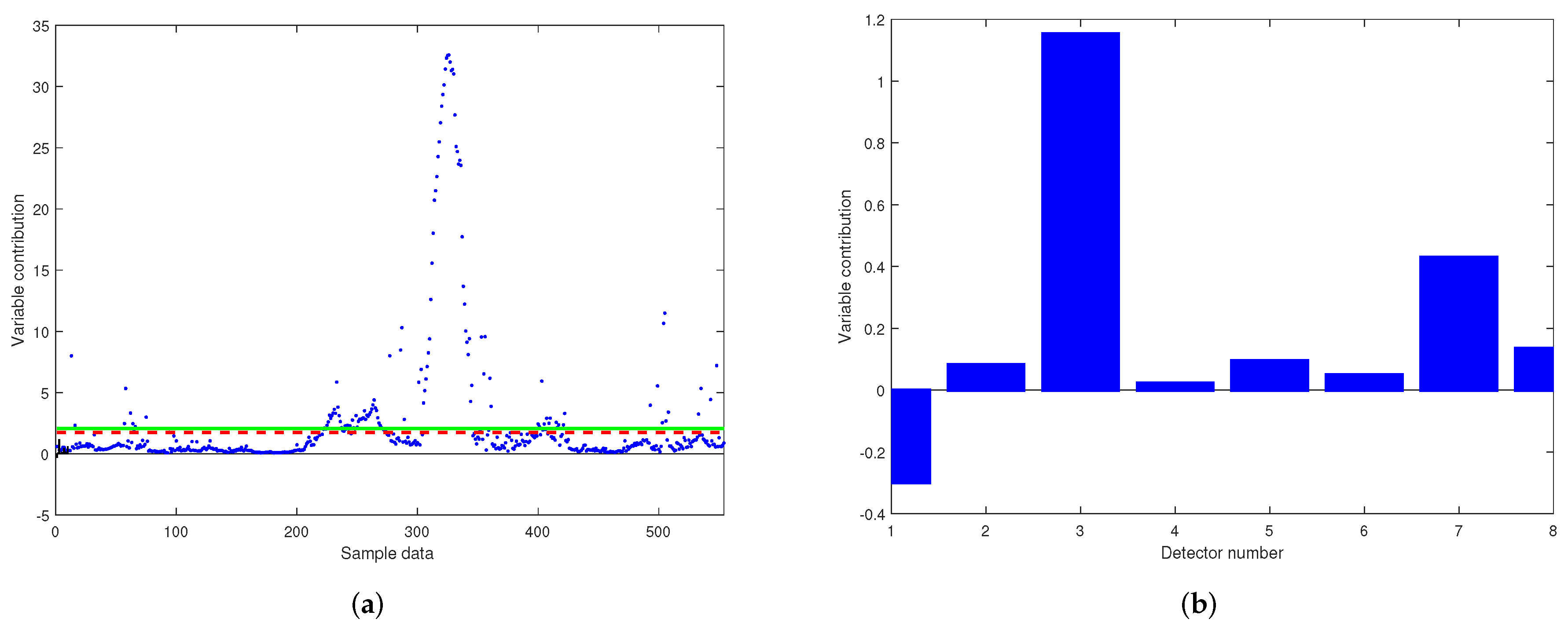
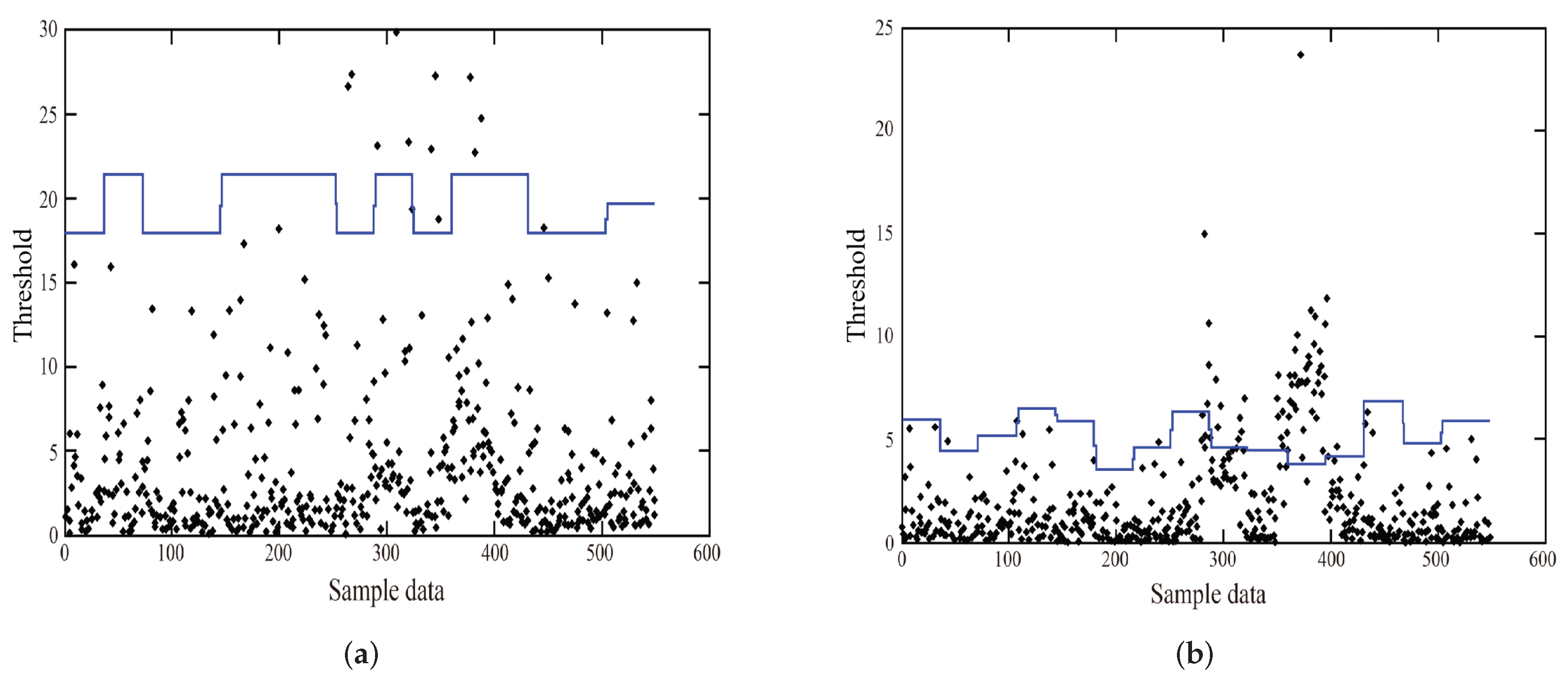
From Figure 7a, it can be found that the data near the sampling point 300–350 appear to be of a more serious fault type. Other sampling points, such as 500, have a different degree of fault data in the vicinity of the sampling point. Compared to Figure 7b, it is known that the No. 3 detector and No. 7 detector have the greatest contribution to the fault data, of which the number 3 detector has a relatively more serious fault. Among them, the real line represents the $T^2$ control limit of 99% of confidence.

In order to verify the advantages of the proposed fault data detection model, each vector of the data to be detected is first decomposed into a wavelet packet, and the principal component analysis is used to model the matrix composed of each node of the wavelet packet decomposition. The wavelet packet energy difference of each node is calculated, and the component of the fault is found to be analyzed by the PCA model, and the location where the data fails under the component can be determined.

4.2. PCA Fault Data Recognition Results

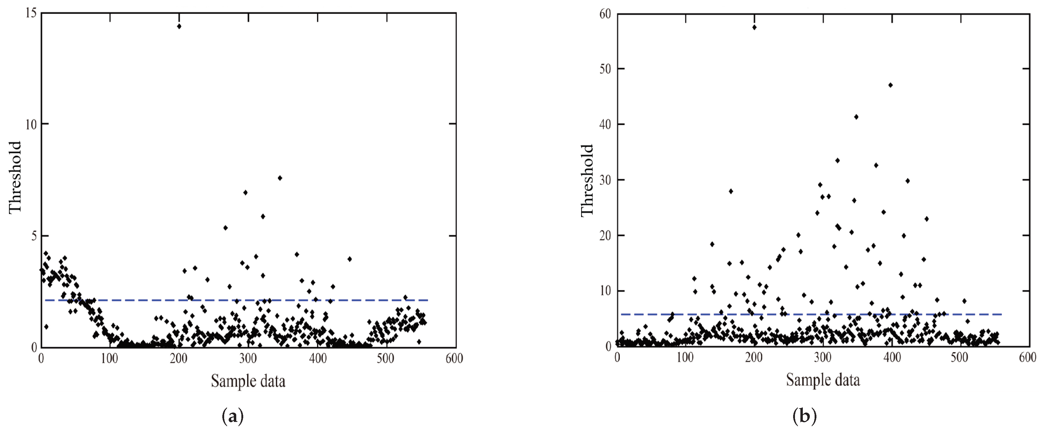
In the $T^2$ and SPE monitoring diagrams, the dotted line indicates that the confidence level is 99% or the SPE control limit parameter. As can be seen from Figure 8, a large number of data points have been misreported. In the monitoring chart, there have been more serious error alarms in the 100 data points at the beginning of the data, and similar problems occurred near 200. Although noise interference is less affected by the SPE monitoring graph, there is a serious misreporting phenomenon.

The fault recognition of the PCA model is caused by the fact that the PCA has no noise interference characteristics, so, if the noise is more intense, the noise information will be treated as the fault information. In addition, traffic flow information is characterized by nonlinear and time-varying characteristics, and the possibility of mutation is relatively large. Therefore, the method of “one size fits all” with various control parameters such as PCA will inevitably lead to errors.

4.3. MSPCA Fault Data Recognition Results

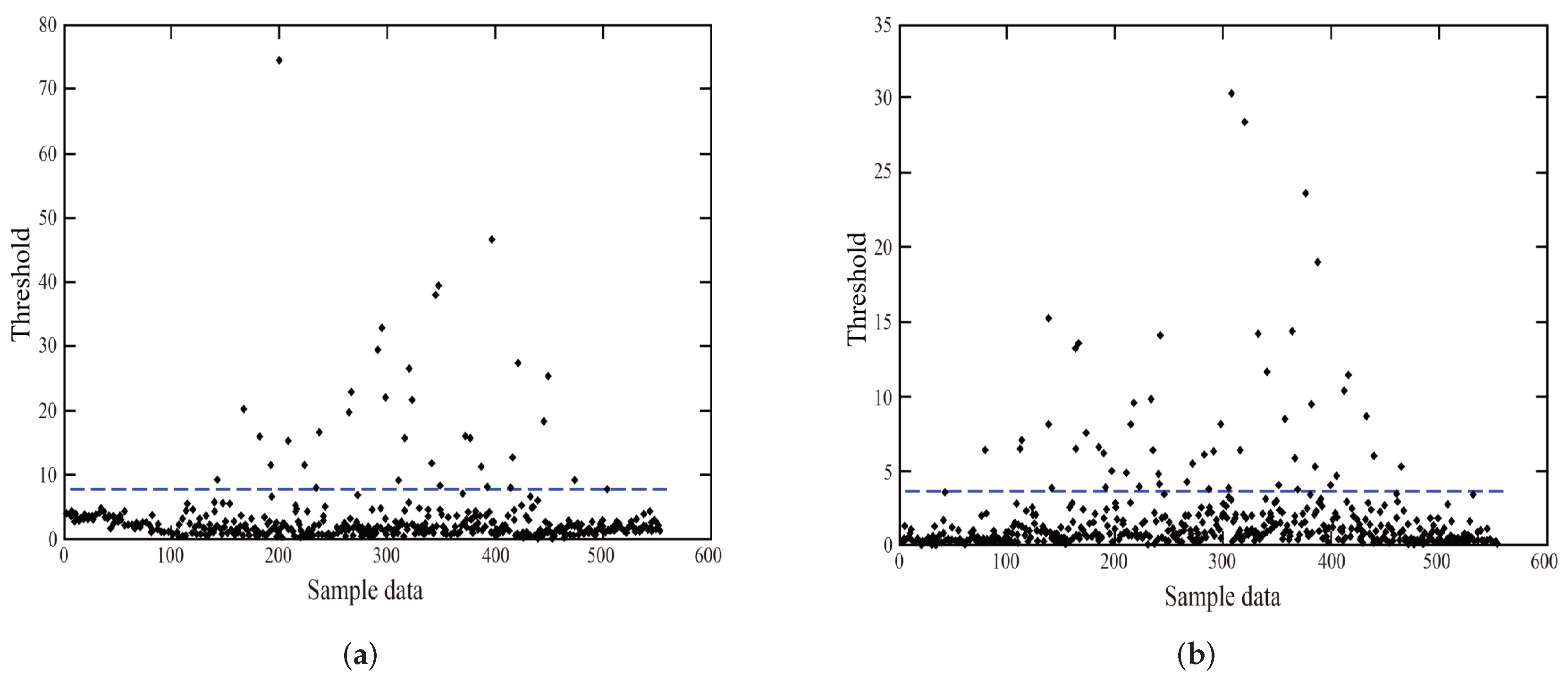
MSPCA combines the wavelet analysis method on the basis of PCA, and carries out unified threshold processing after wavelet decomposition, which has a certain anti-jamming ability to noise. The simulation results are shown in Figure 9. MSPCA can more effectively resist the interference of noise, the false positives of fault are also significantly reduced, but, due to the MSPCA in establishing the main space of atoms and the residual subspace being single, in dealing with traffic flow data, many false positives still appeared.

4.4. Improved MSPCA Fault Data Recognition Results

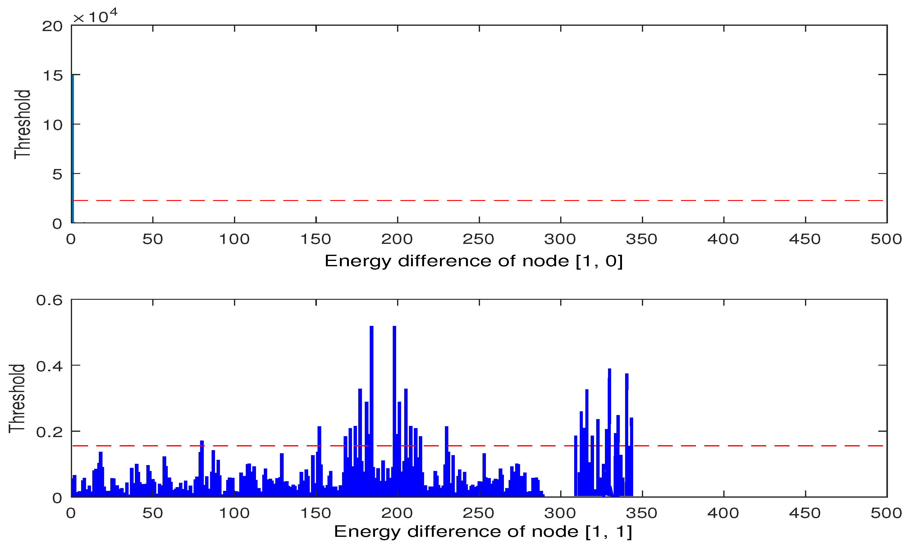
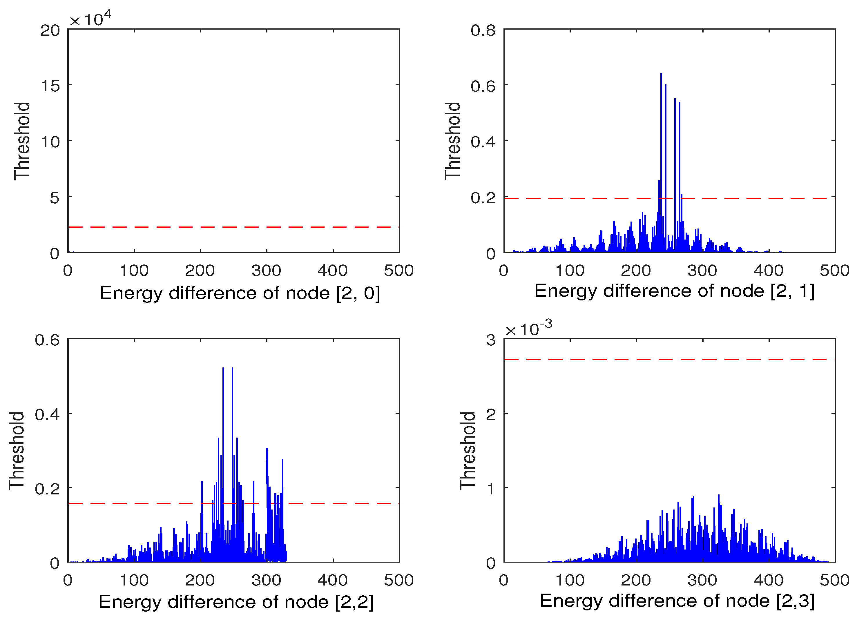
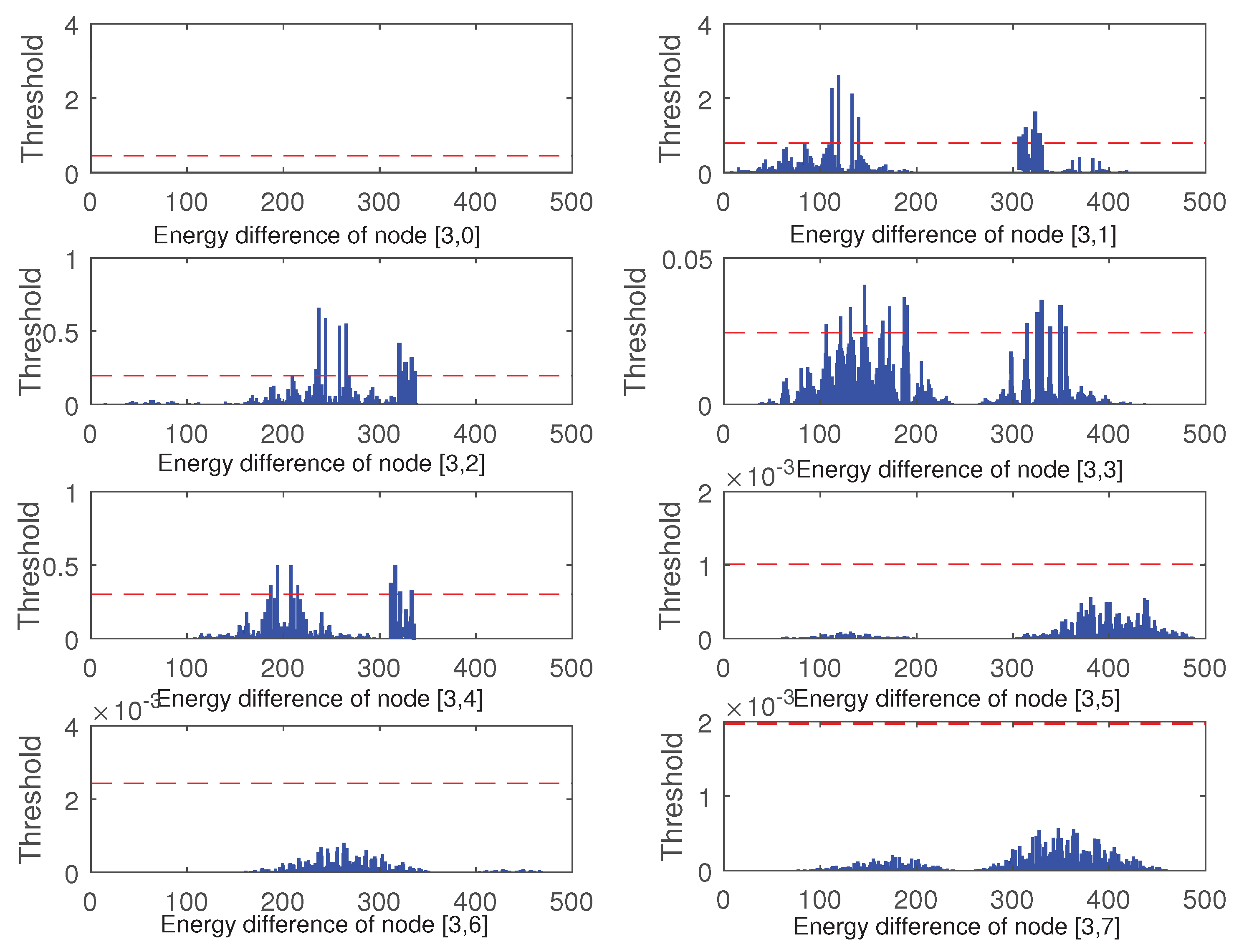
After de-noising by wavelet threshold, the reconstructed signal is decomposed into three-scale wavelet packets. The energy of two nodes is obtained in the first scale, four in the second scale and eight in the third scale. The energy difference between the wavelet packet energy and its corresponding normal data at each scale and the same node at the same scale is calculated, respectively. The result of each scale is shown in Figure 10, Figure 11 and Figure 12.

Figure 11 shows the energy difference of eight vectors decomposed by layer 3 wavelet packet of the detector data. The dashed line represents the energy difference threshold of each component.

In comparison, it can be found that, in Figure 10, no fault information is found in the energy difference of the first layer wavelet packet decomposition signal node [1, 0], and fault information is found in the node [1, 1] near the data point 175–225, 300–350. In Figure 11, the energy of wavelet packet of node [2, 1] detects data faults at about 225–275 data points, and the range of data faults detected by node [2, 2] is about 200–275, 300–350 data points. In the nodes [2, 0] and [2, 3], there is no fault information. At the same time, it can be found that, in the nodes [2, 0], the energy difference is almost zero, which is the same as in the first layer of nodes [1, 0]. Although the energy difference of nodes [2, 3] fluctuates, it does not exceed the set threshold, so it is considered that the change is mainly caused by the noise contained in the data. In Figure 12, node [3, 0] and node [1, 0] have no fault data as in [2, 0]. However, data faults occurred in the vicinity of 150–200, 300–350 in nodes [3, 1], nodes [3, 2], nodes [3, 3], and nodes [3, 4].

Through three-level decomposition of the wavelet packet, the suspected fault location of the data to be checked can be obtained between 150–225 and 275–350 data points. Parameters and principal component modeling analysis are carried out for nodes beyond the threshold at each level, principal component space and residual space are established, and $T^2$ control limit is set. The data with fault information is projected into the principal component space, and the result is shown in Figure 13.

In contrast to the results of the three models, we can find that the improved MSPCA model of this paper can be more effective at making noise reduction in the data, and the error reporting in the malfunction diagnosis is obviously reduced, and it can be obvious from the control limits and the SPE control chart to find the location of the two points of failure. Evaluate the accuracy of each model, as shown in

Table 1. Accuracy comparison of traffic detector fault data identification results.

Model	Statistic	False Alarm Rate	Rate of Missing Report	Accuracy Rate
$PCA$	$T^2$	32.76	8.78	67.21
$PCA$	$SPE$	20.26	4.12	67.21
$MSPCA$	$T^2$	18.45	5.73	78.23
$MSPCA$	$SPE$	12.44	7.87	78.23
$ImprovedMSPCA$	$T^2$	9.12	4.17	89.26
$ImprovedMSPCA$	$SPE$	7.76	0.08	89.26

.

5. Conclusions

In this paper, the traffic flow data collected by traffic detector is studied in fault recognition and data repair. First of all, this paper puts forward the improved MSPCA model, on the basis of traditional MSPCA model, to improve the identification precision of the model, wavelet decomposition to the wavelet packet decomposition, using a wavelet packet energy difference method to test the fault information, and to isolate the fault data. Simulation results show that the improved MSPCA fault data diagnosis model can effectively identify abnormal data.