Dynamic Parameter Identification of a Lower Extremity Exoskeleton Using RLS-PSO

Abstract

The lower extremity exoskeleton is a device for auxiliary assistance of human movement. The interaction performance between the exoskeleton and the human is determined by the lower extremity exoskeleton’s controller. The performance of the controller is affected by the accuracy of the dynamic equation. Therefore, it is necessary to study the dynamic parameter identification of lower extremity exoskeleton. The existing dynamic parameter identification algorithms for lower extremity exoskeletons are generally based on Least Square (LS). There are some internal drawbacks, such as complicated experimental processes and low identification accuracy. A dynamic parameter identification algorithm based on Particle Swarm Optimization (PSO) with search space defined by Recursive Least Square (RLS) is developed in this investigation. The developed algorithm is named RLS-PSO. By defining the search space of PSO, RLS-PSO not only avoids the convergence of identified parameters to the local minima, but also improves the identification accuracy of exoskeleton dynamic parameters. Under the same experimental conditions, the identification accuracy of RLS-PSO, PSO and LS was quantitatively compared and analyzed. The results demonstrated that the identification accuracy of RLS-PSO is higher than that of LS and PSO.

1. Introduction

Over the past decades, advances in electromechanical technology have accelerated the development of lower extremity exoskeletons. Unless otherwise stated, the exoskeleton referred to in this article refers to the lower extremity exoskeleton. The exoskeleton is a device that interacts with the human. The main applications of exoskeletons are physical assistance and rehabilitation [1,2,3,4,5,6,7,8,9,10]. During human–machine interaction, under no circumstances should the exoskeleton directly or indirectly cause injury to the human, either in the routine operation or in fault [11]. Therefore, exoskeleton research should not be confined to mechanical design. It is also challenging and important to improve the performance of the exoskeleton’s controller and to realize compliance control in the process of human–machine interaction [12,13,14]. One of the effective methods to enhance the flexibility of the exoskeleton’s controller is to build an accurate dynamic model [15,16,17,18,19].

Dynamic parameters are used to build the dynamic model of the exoskeleton. There are three main methods to obtain the dynamic parameters of the exoskeleton. First, obtaining the CAD data directly from the manufacturers. This method is not applicable to non-standard products such as exoskeletons. Second, obtaining the CAD data from 3D design software. This method ignores many factors such as the dynamics of hoses and wires, and the internal dynamics of actuators that affect the dynamics of the exoskeleton. Third, obtaining the dynamic parameters through dynamic parameter identification algorithms. This method has high accuracy and requires a series of experiments for data acquisition [20,21,22]. The exoskeleton is made up of many non-standard parts, such as pipes and actuators [6,7,8,9,10], which cause the dynamic parameters of the exoskeleton to fluctuate during working. Obviously, it is difficult to obtain the dynamic parameters from the manufacturers or 3D design software. Therefore, parameter identification algorithms are expected to be an effective way to obtain more accurate dynamic parameters [23,24].

In order to obtain more accurate dynamic parameters, researchers are increasingly paying attention to the application of parameter identification algorithms for the exoskeleton. Researchers have carried out some preliminary research works. Targeting the swing phase [25,26], Justin et al. identified the dynamic parameters of Berkeley Exoskeleton (BLEEX) [21] by means of Least Square (LS) [27,28]. The joint friction coefficients of BLEEX were identified by static experiments, and the inertial parameters [29] were identified by dynamic experiments. The method did not make full use of the non-correlation between the parameters and the linear relationship between the parameters and the parameterized dynamic equations [30,31]. Therefore, the method only identified one parameter in each experiment. Designing a corresponding identification experiment for each parameter was necessary. The process of parameter identification experiment was very complicated, and the friction parameters on the hip joint lost identifiability because of the limited range of motion. The parameter identification accuracy of this method is low. Justin et al. did not compare the identification accuracy of LS with other algorithms. Lin Cong et al. also used LS for dynamic parameters identification of the exoskeleton [16]. However, the identified parameters were only compared with the CAD data calculated by Solidworks. Due to the existence of a large number of non-standard parts [16], it is difficult to prove the accuracy of this method. Jonas [20] proposed a weighted LS method and verified it on an exoskeleton with flexible actuators. The accuracy of the algorithm was also compared with the CAD data of 3D design software. The CAD data could not offer the real value of all the parameters to be identified. Therefore, the accuracy of the method was also not verified. In conclusion, the current parameter identification algorithms for exoskeletons are either complicated, have low accuracy, or lack of quantitative accuracy verification. The identification algorithms are generally based on the LS method. The performance of other parameter identification algorithms in exoskeleton dynamic parameter identification has not been studied. However, Zafer [32] has demonstrated that Particle Swarm Optimization (PSO) has higher identification accuracy than LS on an RX-60 manipulator. Therefore, the introduction of the PSO is expected to improve the accuracy of identification of an exoskeleton’s dynamic parameters.

PSO identifies the parameters through the intelligence of particle swarm and iterative optimization processes [33]. Each dimension represents a parameter to be identified, and the ranges of parameters to be identified are often unknown. In order to avoid losing the real value of parameters, PSO optimization is often carried out in the infinite domain [34]. If the number of iterations is insufficient or the factors are not set properly, the probability that PSO converges to the local minima increases. Taking the local minima as the identification values, the error of the exoskeleton dynamic model will increase. Therefore, it is necessary to reduce the search space of PSO from the infinite domain to the finite domain in advance, to reduce the number of potential local minima within the search space as much as possible.

The fluctuation of exoskeleton parameters provides a possibility to reduce the search space. The approximate range of each parameter can be identified by the recursive identification algorithm before accurate identification of PSO. Recursive least squares (RLS) can identify the fluctuation of parameters. Therefore, the search space of PSO can be defined by RLS. The accuracy of PSO is expected to be further improved with the finite search space. The existing identification algorithms of exoskeleton dynamic parameters are generally based on LS with low accuracy. In this paper, a PSO with search space defined by RLS is designed, named RLS-PSO. The RLS-PSO was verified on a hydraulically driven exoskeleton of the lower extremity. The accuracy of RLS-PSO was compared quantitatively with LS and PSO.

2. Methods

The dynamic equations of the exoskeleton were derived and converted into the form required by the parameter identification algorithm. The physical parameters to be identified were determined by the dynamic equations. According to the linearization requirements of RLS, the physical parameters were converted into inertial parameters [15,16,23,35]. RLS-PSO was designed based on the linearized dynamic equations.

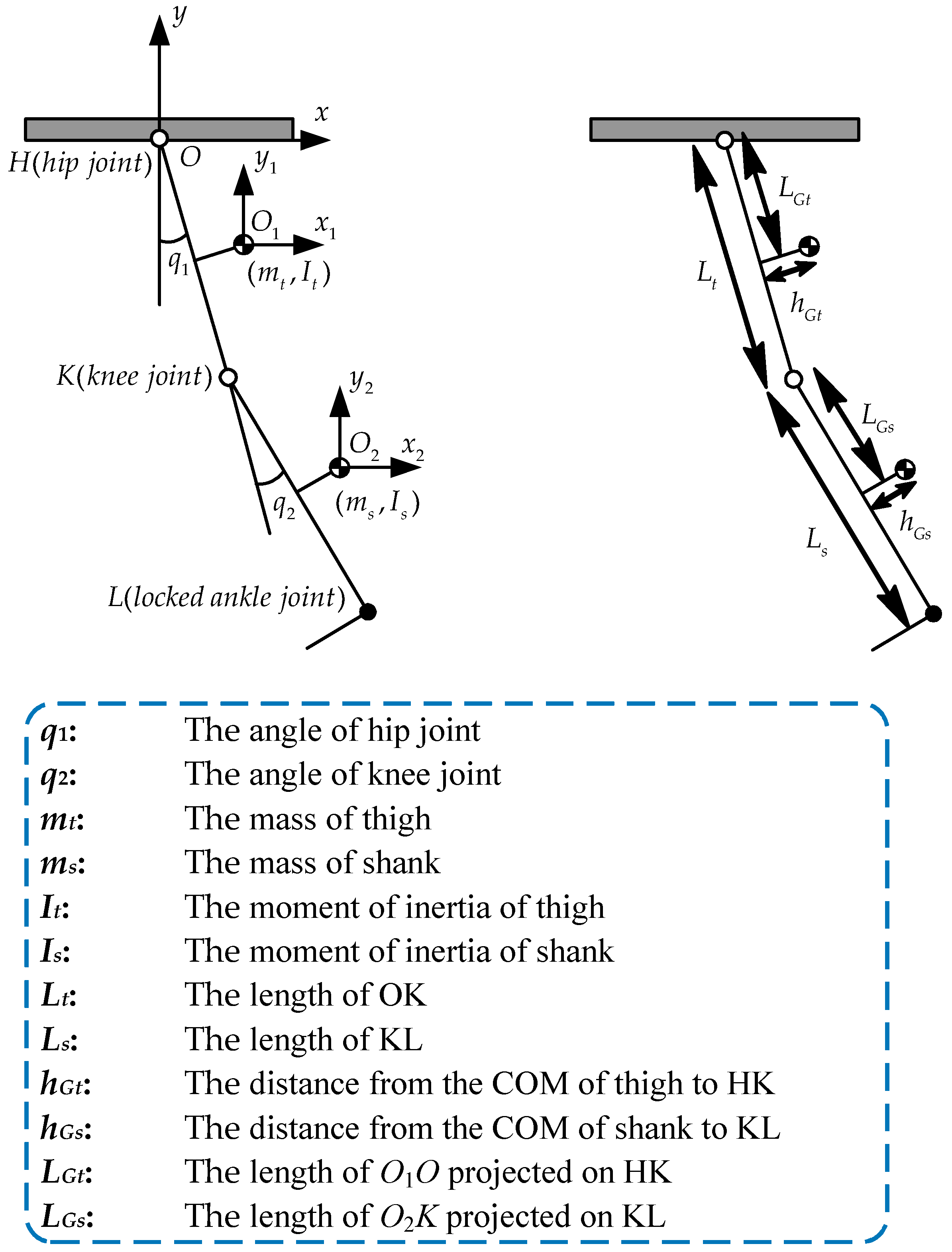
2.1. Parametric Dynamics Equation of Exoskeleton

The RLS-PSO was verified on the active power-assist exoskeleton (APAL) [36] as shown in Figure 1a, which consists of trunk, thigh, shank, and foot modules. As shown in Figure 1b, the trunk and left lower extremity were fixed on the pedestal during the experiment. The right lower extremity was suspended. The hip and knee joints can only swing in the sagittal plane. The forefoot of the exoskeleton was attached to the shank by the fastening band in Figure 1b. The ankle has zero degrees of freedom. The hip and knee joints are driven by hydraulic cylinders, and the exoskeleton is driven only by torque and gravity. The hydraulic actuator of hip joint A is fixed in the trunk and will not affect the dynamic parameters which are related to the thigh and hip joint. Hydraulic cylinder CD drives knee joint B and is fixed on AB. Through the four-linkage mechanism, ABCD, the linear motion of the CD is converted to the rotation of B. The stretching and swinging of the CD cause changes in the position of lower extremity’s center of mass (COM) [36]. Therefore, the dynamic parameters of the thigh and shank fluctuate. The fluctuation was used for defining the search space of PSO.

In the sagittal plane, the right leg of the APAL exoskeleton was simplified into a two-linkage model [37], as shown in Figure 2.

Equation (1) is the dynamic equation of APAL’s lower extremity. Equation (1) was derived by the Lagrange method.

$$\begin{array}{l}{T}_h=[I_s+m_s({(L_s-L_{Gs})}^2-h_{Gs}^2)+I_t+m_t({(L_t-L_{Gt})}^2-h_{Gt}^2)+m_s{L}_t^2+2L_t(m_s(L_s-L_{Gs})\cos q_2-\\ m_s{h}_{Gs}\sin q_2)]{\ddot{q}}_1+[I_s+m_s({(L_s-L_{Gs})}^2-h_{Gs}^2)+L_t(m_s(L_s-L_{Gs})\cos q_2-m_s{h}_{Gs}\sin q_2)]{\ddot{q}}_2+\\ L_t(m_s(L_s-L_{Gs})\sin q_2+m_s{h}_{Gs}\cos q_2)({\dot{q}}_1^2-{({\dot{q}}_1+{\dot{q}}_2)}^2)+g[(m_t(L_t-L_{Gt})+m_s{L}_t)\sin q_1+\\ m_t{h}_{Gt}\cos q_1+m_s(L_s-L_{Gs})\sin (q_1+q_2)+m_s{h}_{Gs}\cos (q_1+q_2)]\\ T_k=[I_s+m_s({(L_s-L_{Gs})}^2-h_{Gs}^2)+L_t(m_s(L_s-L_{Gs})\cos q_2-m_s{h}_{Gs}\sin q_2)]{\ddot{q}}_1+[I_s+m_s((L_s-\\ L_{Gs}{)}^2-h_{Gs}^2)]{\ddot{q}}_2+L_t(m_s(L_s-L_{Gs})\sin q_2+m_s{h}_{Gs}\cos q_2){\dot{q}}_1^2+g[m_s(L_s-L_{Gs})\sin (q_1+q_2)+\\ m_s{h}_{Gs}\cos (q_1+q_2)]\end{array}$$

(1)

where ${\dot{q}}_1$ and ${\dot{q}}_2$ represent the angular velocity of hip and knee joint, respectively, and ${\ddot{q}}_1$ and ${\ddot{q}}_2$ represent the angular acceleration of hip and knee joint, respectively. $T_h$ and $T_k$ represent the hip and knee drive torque required by APAL to complete the trajectory of $q_1$ and $q_2$, respectively. When the lower extremity of APAL is vertically downward, $q_1$ and $q_2$ are zero. The counterclockwise rotation is positive.

Considering the friction on the hip and knee joint, friction torques $T_{f1}$ and $T_{f2}$ were introduced. Equation (2) is the real joint torque $T_1$ and $T_2$.

$$\begin{array}{l}{T}_1=T_h+T_{f1}\\ T_2=T_k+T_{f2}\end{array}$$

(2)

where

$$\begin{array}{l}{T}_{f1}=f_{c1}\mathrm{sgn}({\dot{q}}_1)+f_{v1}{\dot{q}}_1\\ T_{f2}=f_{c2}\mathrm{sgn}({\dot{q}}_2)+f_{v2}{\dot{q}}_2\end{array}$$

$f_{c1}$ and $f_{v1}$ represent the friction parameters of the hip joint, $f_{c2}$ and $f_{v2}$ represent the friction parameter of the knee joint.

Since there are couplings between the physical parameters $I_t$, $I_s$, $m_t$, $m_s$, $L_t$, $L_s$, $L_{Gt}$, $L_{Gs}$, $h_{Gt}$, $h_{Gs}$ in Equation (2), Equation (2) is nonlinear to the above physical parameters. In order to meet the linearization requirements of RLS [38,39], Equation (2) was parameterized to Equation (3). The physical parameters $I_t$, $I_s$, $m_t$, $m_s$, $L_t$, $L_s$, $L_{Gt}$, $L_{Gs}$, $h_{Gt}$, $h_{Gs}$ in Equation (2) were parameterized into a set of inertial parameters $M_{xt}$, $M_{xs}$, $M_{yt}$, $M_{ys}$, $J_t$, $J_s$ that are capable of fully expressing the dynamic characteristics and independent of each other [16,22,23,40]. Equation (3) is linear for the parameters to-be-identified.

$$\begin{array}{l}{T}_1=[J_t+2L_t(M_{xs}\cos q_2-M_{ys}\sin q_2)]{\ddot{q}}_1+[J_s+L_t(M_{xs}\cos q_2-\\ M_{ys}\sin q_2)]{\ddot{q}}_2+L_t(M_{xs}\sin q_2+M_{ys}\cos q_2)[{\dot{q}}_1^2-{({\dot{q}}_1+{\dot{q}}_2)}^2]+\\ g[M_{xt}\sin q_1+M_{yt}\cos q_1+M_{xs}\sin (q_1+q_2)+M_{ys}\cos (q_1+q_2)]+\\ f_{c1}\mathrm{sgn}({\dot{q}}_1)+f_{v1}{\dot{q}}_1\\ T_2=[J_s+L_t(M_{xs}\cos q_2-M_{ys}\sin q_2)]{\ddot{q}}_1+J_s{\ddot{q}}_2+L_t(M_{xs}\sin q_2+\\ M_{ys}\cos q_2){\dot{q}}_1^2+g[M_{xs}\sin (q_1+q_2)+M_{ys}\cos (q_1+q_2)]+\\ f_{c2}\mathrm{sgn}({\dot{q}}_2)+f_{v2}{\dot{q}}_2\end{array}$$

(3)

where

$$\begin{array}{l}{M}_{xt}=m_t(L_t-L_{Gt})+m_s{L}_t\\ M_{yt}=m_t{h}_{Gt}\\ M_{xs}=m_s(L_s-L_{Gs})\\ M_{ys}=m_s{h}_{Gs}\\ J_t=I_s+m_s[{(L_s-L_{Gs})}^2-h_{Gs}^2]+I_t+m_t[{(L_t-L_{Gt})}^2-h_{Gt}^2]+m_s{L}_t^2\\ J_s=I_s+m_s[{(L_s-L_{Gs})}^2-h_{Gs}^2]\end{array}$$

Equation (3) is the linearization dynamic equation of APAL, where $M_{xt}$, $M_{xs}$, $M_{yt}$, $M_{ys}$, $J_t$, $J_s$, $f_{c1}$, $f_{c2}$, $f_{v1}$, $f_{v2}$ are the parameters to-be-identified.

2.2. Design of RLS-PSO Parameter Identification Algorithm

The design of the RLS-PSO was based on Equation (3). The RLS-PSO consists of two parts. First, defining the search space for each parameter. Second, identifying parameters within the search space. The search spaces of the parameters were defined by RLS. The accurate identification of the parameters was implemented by the PSO within the search space.

2.2.1. Establishment of the RLS

As mentioned earlier, the parameters to-be-identified fluctuated due to the movement of the hydraulic actuators. The RLS can identify the time-variant parameters. Therefore, the RLS was adopted to define the fluctuation ranges of $M_{xt}$, $M_{xs}$, $M_{yt}$, $M_{ys}$, $J_t$, $J_s$, $f_{c1}$, $f_{c2}$, $f_{v1}$, $f_{v2}$. The fluctuation ranges of $M_{xt}$, $M_{xs}$, $M_{yt}$, $M_{ys}$, $J_t$, $J_s$, $f_{c1}$, $f_{c2}$, $f_{v1}$, $f_{v2}$ form a 10-dimension search space. In order to facilitate computer programming and calculation, Equation (3) was converted into matrix form as Equation (4).

$$\begin{array}{l}{T}_1=H_h(q_1,{\dot{q}}_1,{\ddot{q}}_1,q_2,{\dot{q}}_2,{\ddot{q}}_2)X\\ T_2=H_k(q_1,{\dot{q}}_1,{\ddot{q}}_1,q_2,{\dot{q}}_2,{\ddot{q}}_2)X\end{array}$$

(4)

where

$$\begin{array}{l}X={[M_{xt},M_{yt},J_t,f_{c1},f_{v1},M_{xs},M_{ys},J_s,f_{c2},f_{v2}]}^T\\ H_h=[g\sin q_1,g\cos q_1,{\ddot{q}}_1,sgn({\dot{q}}_1),{\dot{q}}_1,2L_t{\ddot{q}}_1\cos q_2+L_t{\ddot{q}}_2\cos q_2+\\ L_t\sin q_2[{\dot{q}}_1^2-{({\dot{q}}_1+{\dot{q}}_2)}^2]+g\sin (q_1+q_2),-2L_t{\ddot{q}}_1\sin q_2-L_t{\ddot{q}}_2\sin q_2+\\ L_t[{\dot{q}}_1^2-{({\dot{q}}_1+{\dot{q}}_2)}^2]\cos q_2+g\cos (q_1+q_2),{\ddot{q}}_2,sgn({\dot{q}}_1),{\dot{q}}_1]\\ H_k=[0,0,0,0,0,L_t{\ddot{q}}_1\cos q_2+L_t{\dot{q}}_1^2\sin q_2+g\sin (q_1+q_2),\\ -L_t{\ddot{q}}_1\sin q_2+L_t{\dot{q}}_1^2\cos q_2+g\cos (q_1+q_2),{\ddot{q}}_1+{\ddot{q}}_2,sgn({\dot{q}}_2),{\dot{q}}_2]\end{array}$$

In Equation (4), $H_h$ and $H_k$ represent motion information vectors. X represents the parameter vector. While the hip and knee joints are swinging, the hip joint generates a torque to counteract the interference caused by the swing of knee joint to complete the target trajectory. Similarly, the knee joint also generates a torque that counteracts the interference caused by the swing of hip joint. Equation (5) was derived from Equation (4). Equation (5) is the equation of the LS.

$$\begin{array}{l}X={(H_i^T{H}_i)}^{-1}{H}_i^T{T}_j\\ (i=h,k;j=1,2)\end{array}$$

(5)

X was identified in each iteration of RLS to define the fluctuation range of X. Therefore, Equation (5) was converted into a recursive form as Equation (6). Equation (6) is the RLS.

$$\{\begin{array}{l}K=P(kg-1)\ast H_i/(H_i^T\ast P(kg-1)\ast H_i+1/weight)\\ new=T_j(kg)-H_i^{T}X(kg)\\ X(kg+1)=X(kg)+K\ast new\\ P(kg)=1/weight\ast (eye(2)-K\ast H_i^T)\ast P(kg-1)\\ eye(2)=\left(\begin{array}{cc}1& 0\\ 0& 1\end{array}\right)\\ (kg>1,kg\in N+;i=h,k;j=1,2)\end{array}$$

(6)

where kg represents the number of iterations of RLS. The detailed derivation processes of Equation (6) and the principle of RLS can be referred to [41]. The fluctuation ranges of X given by the RLS is the search space of PSO.

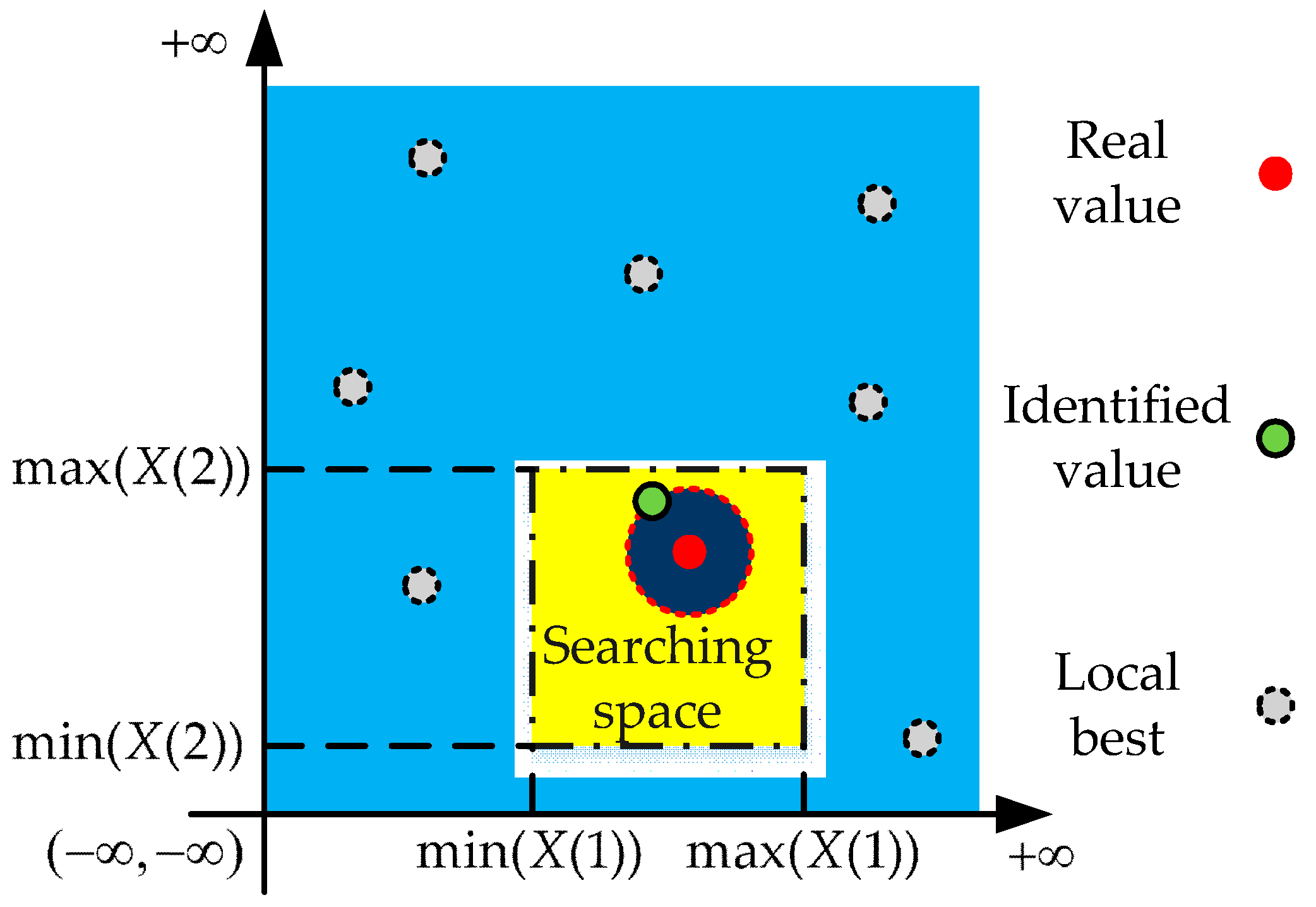
2.2.2. PSO with a Finite Search Space

PSO is an algorithm based on particle swarm intelligence. PSO is mainly used for parameter identification and optimization. In each iteration, PSO adjusts the direction and distance of the flight based on the best solution of the particle’s own motion trajectories and the best solution of the whole particles’ motion trajectories. Through continuous iterations, PSO finally converges into the neighborhood of the global minima. Under the same parameters, defining the search space is expected to improve the identification accuracy of PSO.

Take the identification of $X(1)$ and $X(2)$ as an example. As shown in Figure 3, when the ranges of $X(1)$ and $X(2)$ are unknown, the search space of PSO is 2-dimensional (n is the number of parameters to-be-identified) infinite domain (the blue rectangle). If the number of iterations is insufficient or the settings are inappropriate, the PSO will converge to the local minima. In order to solve this problem, the X’s search space (the yellow dotted line rectangle) defined by the RLS is adopted to replace the infinite domain. The search space of PSO is greatly reduced. Under the same number of iterations, PSO is more likely to converge into a small neighborhood of real values (the red dotted circle). Since a much smaller search space is defined, a large number of local minima are excluded from the new search space.

Linearly decreasing inertia weight was adopted in PSO. At the beginning of the iteration, the global search performance of PSO was good. PSO converged to the vicinity of the global minima quickly. In the latter part of the iteration, the local search performance of PSO was good, so as to accurately approximate the global minima.

The PSO initialized the position $S_{\mathrm{i}}^1$ and velocity $V_i^1$ of the particles by Equation (7).

$$\begin{array}{l}{S}_{\mathrm{i}}^1=\min (S_{\mathrm{i}}^1)+rand\times [\max (S_{\mathrm{i}}^1)-\min (S_{\mathrm{i}}^1)]\\ V_i^1=\min (V_i^1)+rand\times [\max (V_i^1)-\min (V_i^1)]\\ rand\in [0,1],(i=1,2,\dots ,10)\end{array}$$

(7)

where $\max (S_{\mathrm{i}}^1)$ and $\min (S_{\mathrm{i}}^1)$ represent the maximum and minimum value of $X(i)$’s search space, respectively. $\max (V_i^1)$ and $\min (V_i^1)$ represent the maximum and minimum value of $X(i)$’s velocity, respectively. To ensure that the particles were always iteratively searched within the search space, once a particle’s position or velocity exceeded the given range, the value was reset to its nearest maximum or minimum. The PSO performed $G$ iterations. In the kg$(kg>1,kg\in N+)$ iteration, the PSO updated the positions and velocities of the particles by Equation (8).

$$\begin{array}{l}{V}_i^{kg}=w(t)\times V_i^{kg-1}+c_1{r}_1(p_{gb}^{kg-1}-S_i^{kg-1})+c_2{r}_2(p_{i\_lb}^{kg-1}-S_i^{kg-1})\\ S_i^{kg}=S_i^{kg-1}+V_i^{kg},(r_1=rand,r_2=rand)\\ w(kg)=w_{max}-\frac{kg}{G}(w_{max}-w_{min})\\ rand\in [0,1],(i=1,2,\dots ,10)\end{array}$$

(8)

where $S_i^{kg}$ and $V_i^{kg}$ represent the position and velocity of particle $X(i)$ in the $kg$ iteration, respectively. $r_1$ and $r_2$ represent the normal distribution random numbers between [0, 1]. $c_1$ and $c_2$ represent the learning factor of the particle. $w(kg)$ represents the inertia time-variant weight in the $kg$ iteration. $p_{gb}^{kg-1}$ and $p_{i\_lb}^{kg-1}$ represent the global minima of the $kg-1$ iteration and the local minima of the particle $X(i)$, respectively. Equations (7) and (8) are the PSO with a finite search space. Detailed derivation and principle of PSO can be found in [42].

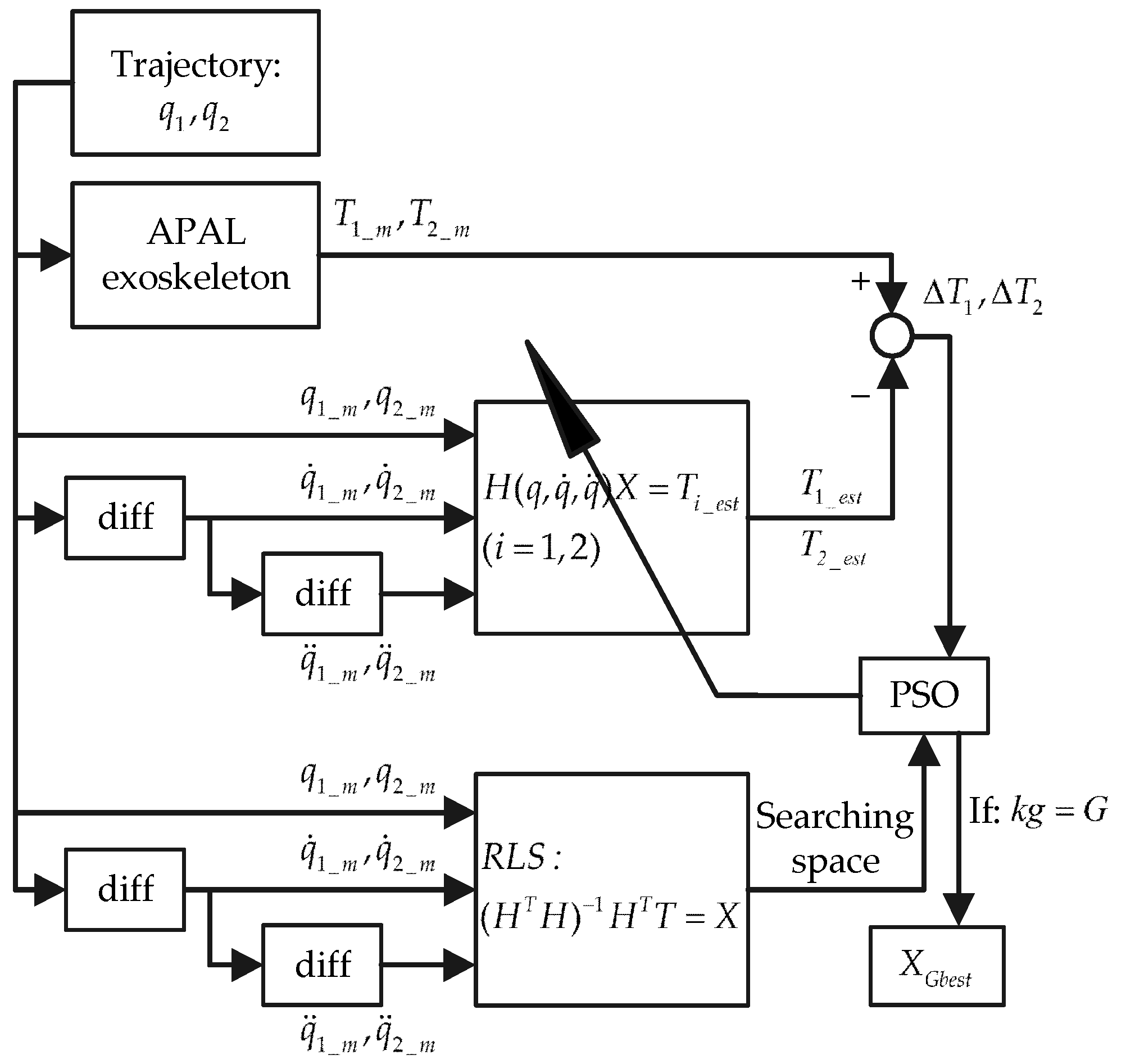
2.2.3. Flowchart of RLS-PSO

Based on the established RLS and PSO, RLS-PSO was designed. The hip and knee joints of APAL swing according to the hip and knee trajectories $q_1$ and $q_2$, respectively. The sensors measure hip and knee torques represented by $T_{1\_m}$ and $T_{2\_m}$, respectively. Hip and knee angles respectively represented by $q_{1\_m}$ and $q_{2\_m}$ are also measured by sensors. The hip and knee joints angular velocities respectively represented by ${\dot{q}}_{1\_m}$ and ${\dot{q}}_{2\_m}$ are calculated by forward difference. The hip and knee joints angular accelerations respectively represented by ${\ddot{q}}_{1\_m}$ and ${\ddot{q}}_{2\_m}$ are calculated by quadratic forward difference. Figure 4 is the flowchart of RLS-PSO.

The steps of RLS-PSO are as follows:

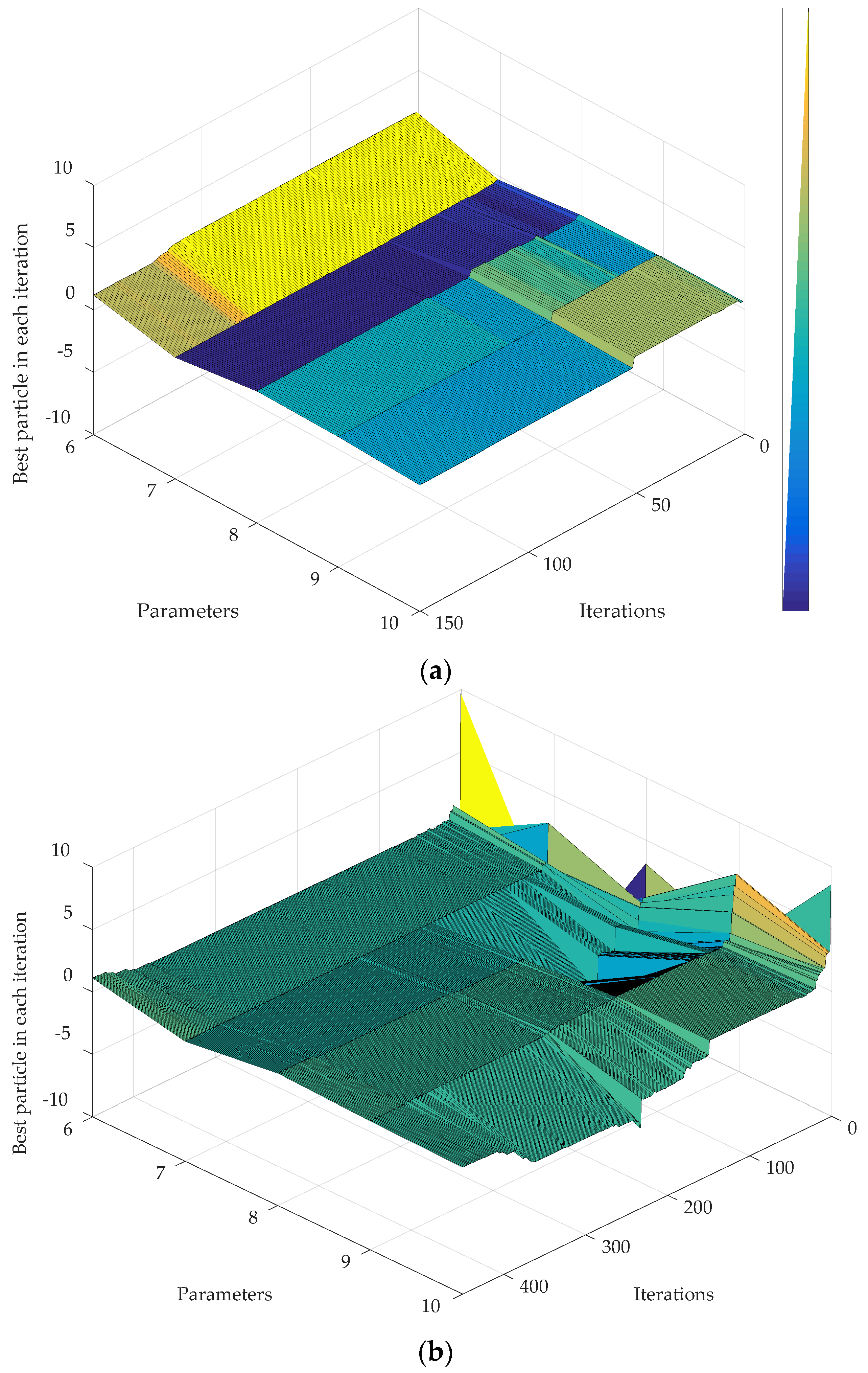
• RLS identifies the fluctuation range of each parameter in X by Equation (6), thereby defining the search space of PSO;
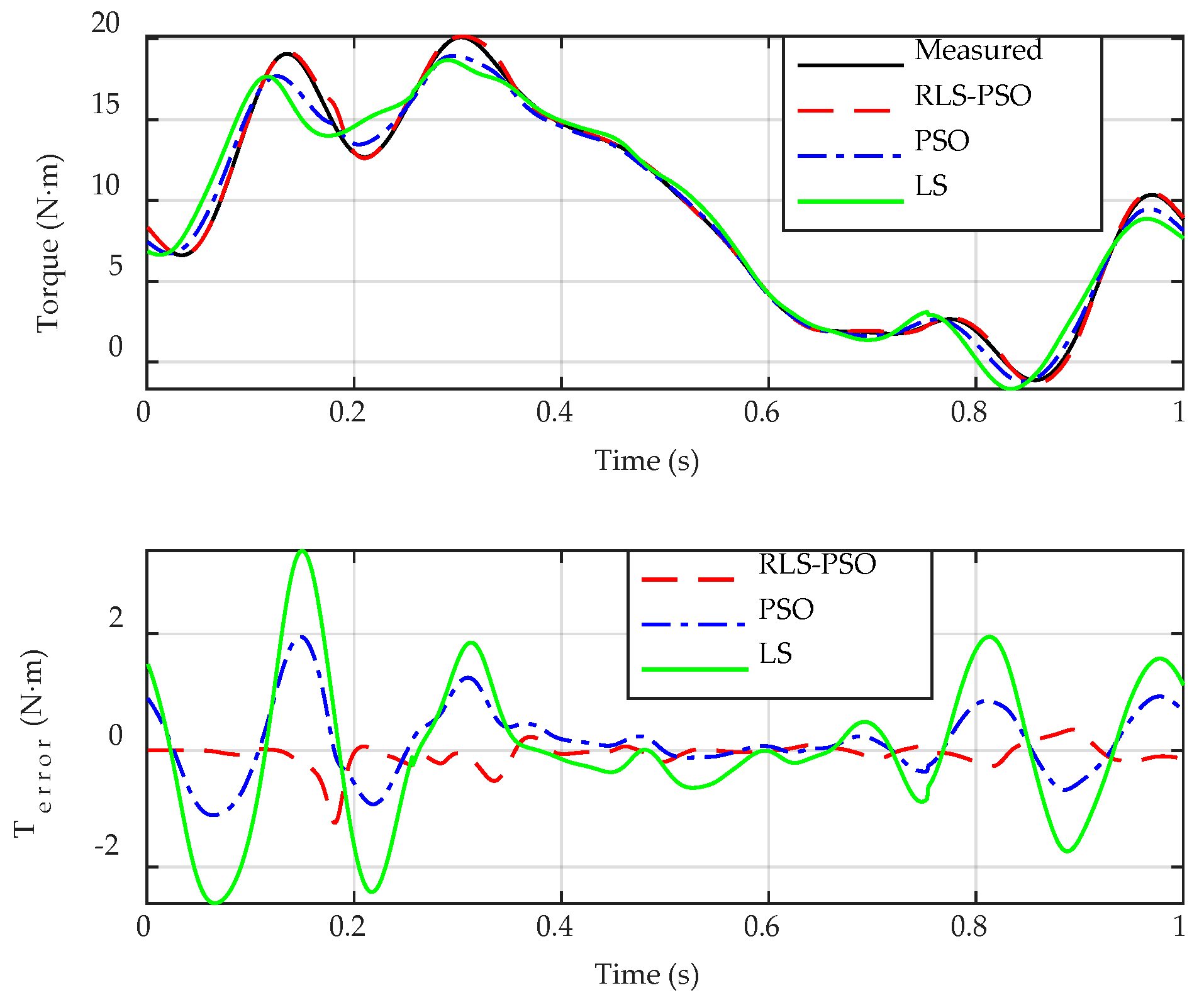
• Within the search space defined by the RLS, the PSO optimizes X by Equations (7) and (8). The estimated values of the hip and knee torques respectively represented by $T_{1\_est}$ and $T_{2\_est}$ are calculated by substituting X identified in each iteration into Equation (4). $T_{1\_est}$ and $T_{2\_est}$ are subtracted from $T_{1\_m}$ and $T_{2\_m}$, respectively. The absolute values of the differences are $\Delta T_1$ and $\Delta T_2$, respectively. In each iteration, the optimization goal of the PSO is: $\Delta T_1+\Delta T_2<\epsilon$, $\epsilon \to 0+$;
• When the iteration reaches G times or $\Delta T_1+\Delta T_2<\epsilon$ ($\epsilon ={10}^{-2}$, $G=10000$), the PSO stops searching and the global minima $X_{Gbest}$ is the identified parameter vector.

3. Data Acquisition and Discussion

In order to verify the validity of the RLS-PSO, the data acquisition of $H_h$, $H_k$, $T_1$, and $T_2$ under given trajectories was completed on the APAL. Based on the identified torque, the identification accuracy of LS, PSO, and RLS-PSO has been compared quantitatively. All the parameter identification algorithms were compiled in Python.

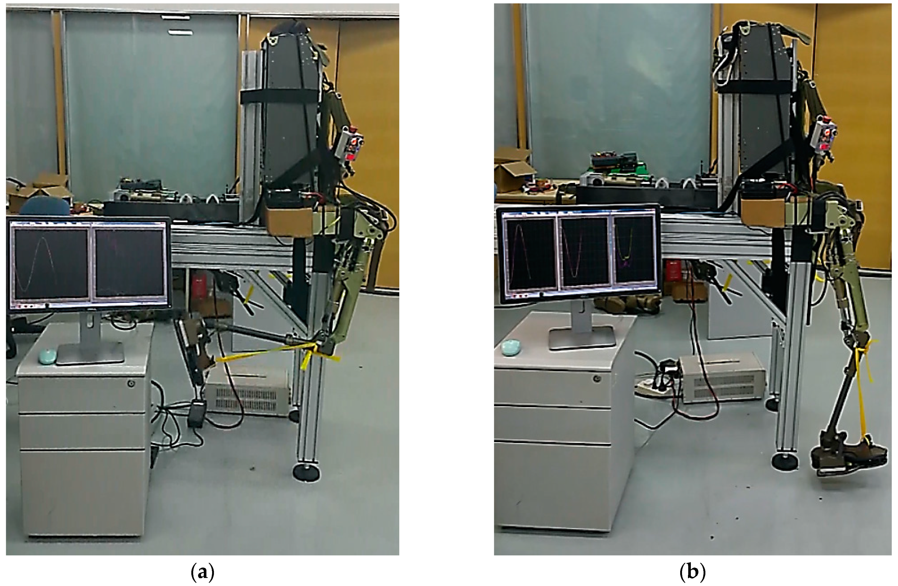
3.1. Data Acquisition

The acceleration signal is affected by the vibration of the pedestal [42], resulting in an increase in the identification error. The vibration caused by the simultaneous swing of the hip and knee joint is larger than the vibration of the single knee joint. Therefore, in order to reduce the influence of the vibration of the pedestal, a segmental identification strategy was adopted. First, the hip joint was fixed. The knee joint swung. At this time, the vibration of the pedestal was relatively small. The identification of $X(6:10)$ was completed first. By then, the hip and knee joints swung together to complete the identification of $X(1:5)$. The flowchart of segment identification is shown in Figure 5. There are three steps of the segmental identification strategy:

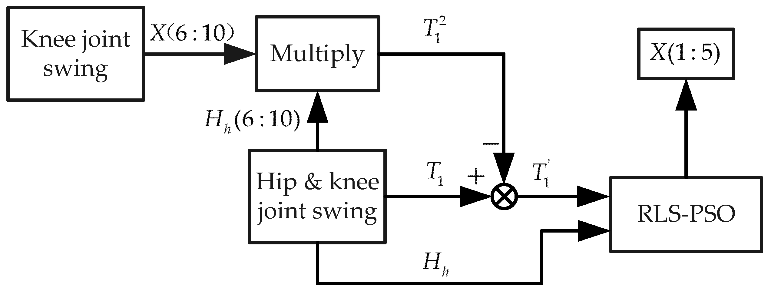
• The hip joint is fixed. The knee joint follows the target trajectory. $T_2$ and $H_k$ are acquired. Substitute $T_2$ and $H_k(6:10)$ into Equation (6) to define the range of $X(6:10)$ as the search space of the PSO. The identification of $X(6:10)$ is completed by Equation (7) and (8);
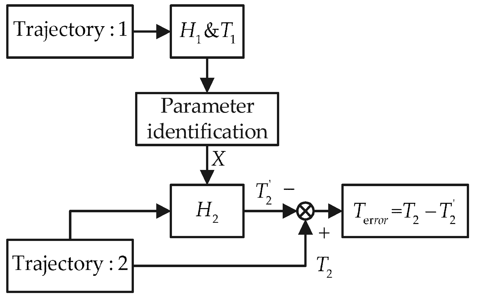
• Both the hip and knee joints follow the target trajectory. After that, $H_h$ is acquired. Substitute $H_h(6:10)$ and $X(6:10)$ into equation (9) to calculate $T_1^2$. $T_1^2$ is the torque generated by the hip joint to resist the interference of the swing on the knee joint. $T_1$ is calculated by equation (4). $T_1^{\prime }$ is the difference between $T_1$ and $T_1^2$;

  $$T_1^2=H_h(6:10)X(6:10)$$

  (9)
• Substituting $H_h$ and $T_1^{\prime }$ into Equation (6) defines the range of $X(1:5)$ as the search space of the PSO. $X(1:5)$ is identified by Equations (7) and (8).

The trajectories of the hip and knee joints of APAL are shown in

Table 1. Trajectories of hip and knee joints.

No.	Hip Trajectory	Knee Trajectory
1	−10	45 − 30sin(2πt)
2	−10	60 − 30sin(2πt)
3	−30 − 30sin(2πt)	75 − 30sin(2πt)
4	−45 − 30sin(2πt)	60 + 30sin(2πt)

. No.1 and No.2 are the trajectories of knee joint swing experiments. No.3 and No.4 are the trajectories of the hip and knee joints swing experiments.

As shown in Figure 6, the APAL’s trunk and left lower extremity were fixed to the pedestal and the right lower extremity was suspended. The PID control law was adopted to make the hip and knee joint track the given trajectories in Table 1. The sampling frequency was 1000 Hz. When people walk and run, the frequency of motion is 0.85~5 Hz [43,44]. According to the sampling theorem, the measured and calculated data were zero-phase filtered with a 10 Hz low-pass filter. Compared to differential filters, zero-phase filters do not cause signal phase shifts and waveform distortion. Therefore, a zero-phase filter was adopted to reduce the effect of waveform distortion on the accuracy of the identification.

The tracking accuracy and response time of the hip and knee joints in the experiment are shown in

Table 2. Mean of tracking accuracy and response time of APAL.

Performance Index	Hip Angle	Knee Angle
Tracking accuracy (°)	0.0217	0.0358
Response time (s)	0.6806	0.9725

.

Table 2 shows that APAL has good accuracy and response performance. The hip and knee joints accurately tracked the given trajectories in Table 1. The measured data can be adopted for parameter identification.

3.2. The Identification of Parameters

In order to verify the accuracy of the RLS-PSO, a quantitative accuracy evaluation method was adopted. In order to verify the effectiveness of RLS-PSO in improving the accuracy of exoskeleton parameter identification, the identification accuracy of LS, PSO, and RLS-PSO was quantitatively compared. To this end, the method in Figure 7 was designed which can quantitatively evaluate the accuracy of the identification algorithm.

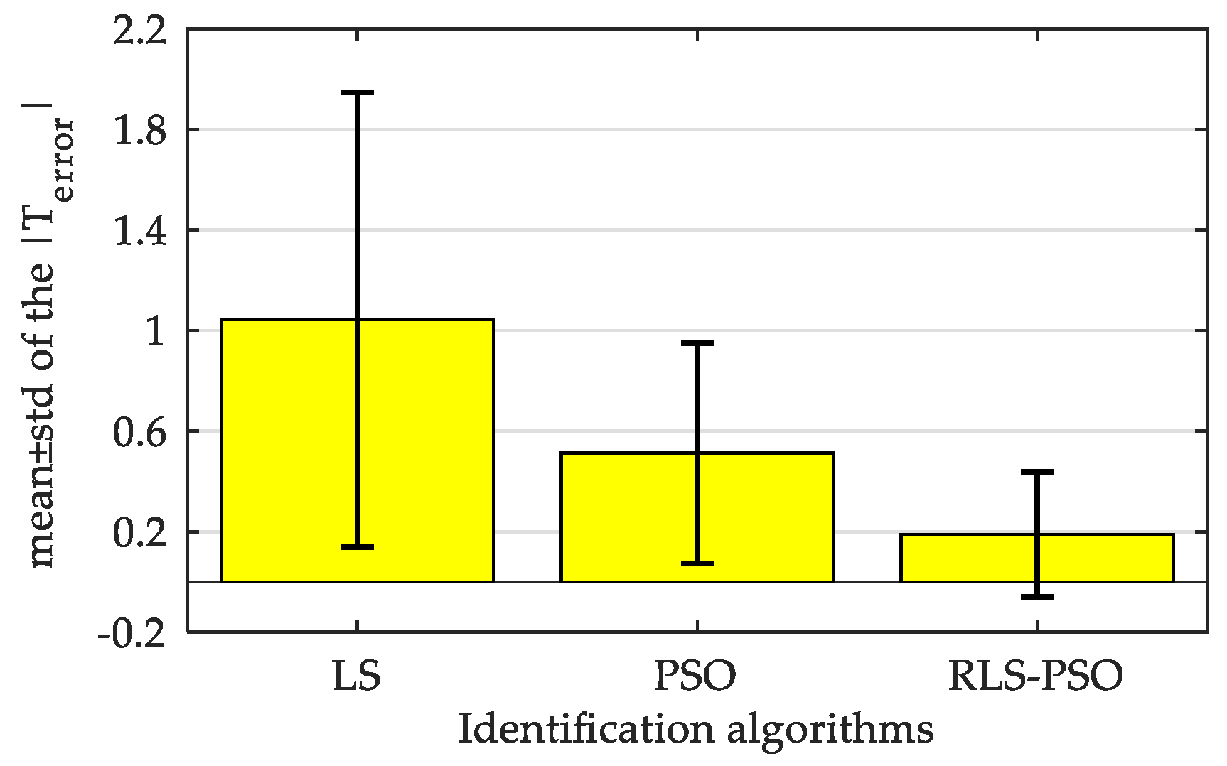
3.2.1. Quantitative Evaluation Method for Identification Accuracy

Since the real values of X are unknown, the accuracy of the identification algorithm cannot be evaluated by comparing the identification values with the real values. The original intention and application of exoskeleton parameter identification is to calculate joint torques. Therefore, using the error between the identified torque and the measured torque to evaluate the identification accuracy is consistent with the original intention and application of exoskeleton parameter identification. The method of evaluating identification accuracy by the error between identified torque and measured torque has been verified and applied [21,32]. Ghan et al. evaluated the identification accuracy by the agreement between the identified torque and measured torque [21]. Bing et al. used the comparison of identified torque and measured torque for evaluating the identification accuracy and comparing between PSO and LS. In summary, when the parameters are unknown, it is feasible and effective to evaluate identification accuracy by the errors of identified torque and measured torque in the exoskeleton parameter identification whose original intention and application is the calculation of joint torques. Therefore, this method was also adopted in this paper to evaluate identification accuracy as shown in Figure 7. The method can quantitatively evaluate the accuracy of the identification algorithm. Take the experiment in Figure 6a as an example. The identification of X was implemented based on the data measured from trajectory 1. $H_2$ was acquired in trajectory 2. $T_2^{\prime }$ was calculated from Equation (4). The difference between $T_2^{\prime }$ and $T_2$ was the torque identification error $T_{error}$.

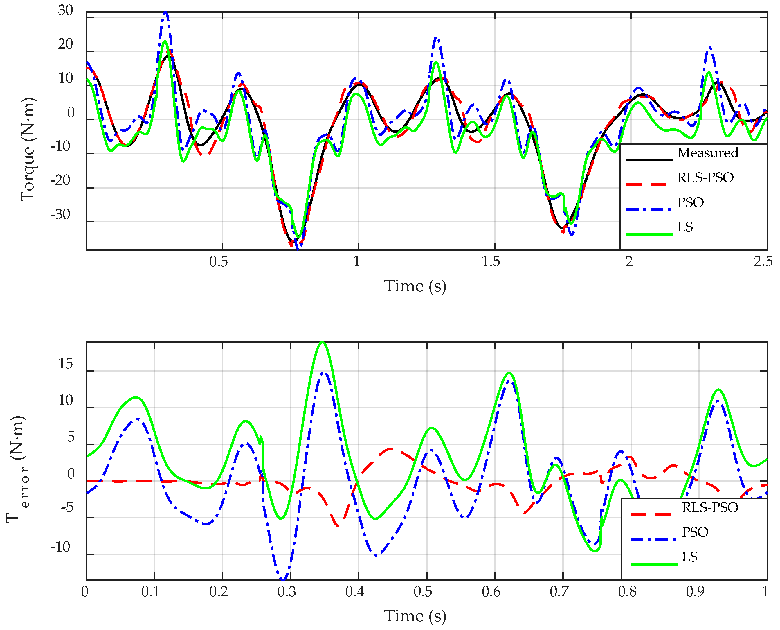
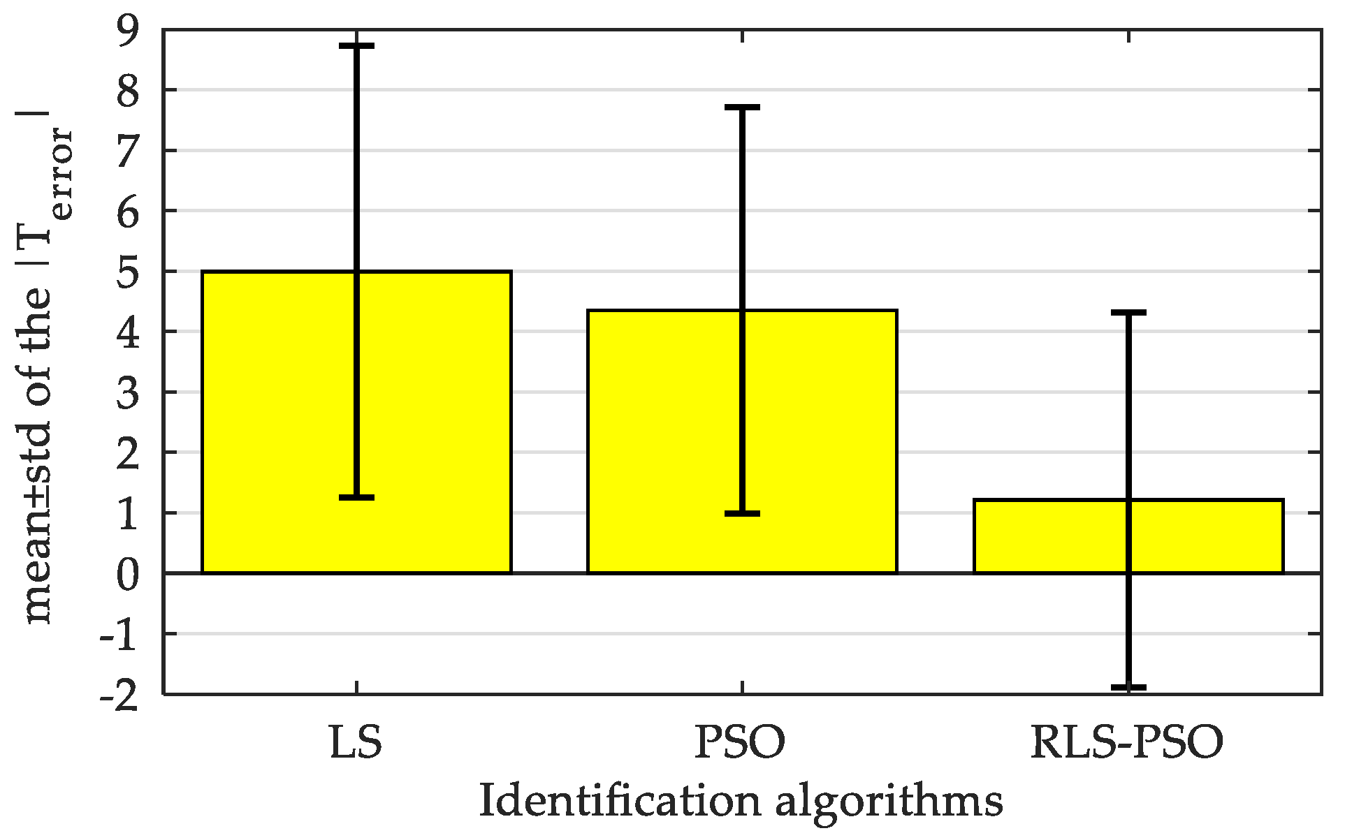
3.2.2. Quantitative Analysis of RLS-PSO Identification Accuracy

The identification of $X(6:10)$ was implemented by the data acquired from trajectory 1. The search space of $X(6:10)$ in

Table 3. The search space of $X(6:10)$ defined by RLS.

$\mathit{X}(6)$	$\mathit{X}(7)$	$\mathit{X}(8)$	$\mathit{X}(9)$	$\mathit{X}(10)$
0.79~1.79	−0.98~0.18	0.39~0.91	0.01~1.13	0.02~3.15

was defined by RLS. $X(6:10)$ was identified by LS, PSO, and RLS-PSO, respectively. The identification values are shown in

Table 4. The identified values of $X(6:10)$.

Type	$\mathit{X}(6)$	$\mathit{X}(7)$	$\mathit{X}(8)$	$\mathit{X}(9)$	$\mathit{X}(10)$
LS	1.3859	−0.8267	0.7019	0.0943	0.2907
PSO	1.2199	−0.4016	0.5906	0.3323	0.1830
RLS-PSO	1.1822	−0.2808	0.5655	0.4406	0.1020

. In each iteration of PSO and RLS-PSO, the best particle which obtains the minimum error is selected. The best particle convergence of PSO and RLS-PSO is shown in Figure 8. The LS does not have iteration processes, so LS is not shown in Figure 8.

Trajectory 2 was the reference group, and the identification values of $X(6:10)$ was quantified by the quantitative evaluation method in Figure 7. Figure 9 is a comparison of the identified torque, the measured torque, and the torque error $T_{error}$.

The absolute values of $T_{error}$ were averaged. The mean ± std of the absolute torque error of LS as shown in Figure 10 is 1.0427 ± 0.9047 Nm. The mean ± std of the absolute torque error of the PSO is 0.5126 ± 0.4386 Nm. The mean ± std of the absolute torque error of the RLS-PSO is 0.1887 ± 0.2475 Nm. As shown in Figure 10, it is clear that the most accurate $X(1:5)$ was identified by the RLS-PSO. Under the same conditions, the accuracy of RLS-PSO is improved by 81.9% compared with LS, and the accuracy of RLS-PSO is improved by 63.19% compared with PSO.

Similarly,

Table 5. The search space of $X(1:5)$ defined by RLS.

$\mathit{X}(1)$	$\mathit{X}(2)$	$\mathit{X}(3)$	$\mathit{X}(4)$	$\mathit{X}(5)$
5.38~11.64	2.34~5.20	2.01~4.25	0.10~7.88	0.01~1.70

is the search space of $X(1:5)$ defined by RLS. The segmental identification strategy was adopted to identify $X(1:5)$.

Table 6. The identified values of $X(1:5)$.

	$\mathit{X}(1)$	$\mathit{X}(2)$	$\mathit{X}(3)$	$\mathit{X}(4)$	$\mathit{X}(5)$
LS	6.5124	2.4481	2.4996	1.7285	0.0245
PSO	7.9970	3.4969	2.9922	1.5914	0.0752
RLS-PSO	7.4433	3.1788	2.8413	1.7285	0.0372

is the identified values of $X(1:5)$. The best particle convergence of PSO and RLS-PSO is shown in Figure 11.

Figure 12 shows the identified torque, measured torque, and torque error $T_{error}$. The mean ± std of the absolute torque error of LS as shown in Figure 13 is 4.9922 ± 3.7366 Nm. The mean ± std of absolute torque error of PSO is 4.3516 ± 3.3602 Nm. The mean ± std of absolute torque error of RLS-PSO is 1.2128 ± 3.100 Nm. The RLS-PSO obsessed the best accuracy. Compared with the LS, the accuracy of the RLS-PSO is improved by 75.70%. Compared with the PSO, the accuracy of the RLS-PSO is improved by 72.13%.

In Figure 11, the number iterations are 120 and 280 for RLS-PSO and PSO, respectively. Obviously, the convergence rate of RLS-PSO is larger than that of PSO.

It can be seen from Figure 10 and Figure 13 that the accuracy of RLS-PSO is significantly higher than LS and PSO. This result shows that under the same conditions, pre-defining the search space of PSO through RLS can effectively improve the identification accuracy of PSO.

Compared with the LS adopted by BLEEX, RLS-PSO does not require static experiments, which not only reduces the complexity of the experiments but also ensures the accuracy of dynamic parameter identification. The hydraulic drive units caused fluctuations in the dynamic parameters during the movement of the exoskeleton. In order to solve this problem, the fluctuation range of each parameter to-be-identified was defined by RLS and used as the search space of PSO. Accurate parameter identification was achieved by PSO in the search space. RLS-PSO converted the problem from the time-variant of the parameters to the optimization of the parameters. It not only solved the time-variant problem of parameters, but also reduced the potential local minima of PSO in the infinite domain. Under the same experimental condition, compared with LS and PSO, RLS-PSO greatly improved the identification accuracy.

Comparing Figure 10 and Figure 13, it can be seen that the identification accuracy of $X(6:10)$ is higher than that of $X(1:5)$. The main reason for this phenomenon is that the large inertia of the thigh and shank has a larger effect on the pedestal than the shank only. As the pedestal’s vibration increased, the interference of the angular acceleration signal increased. In order to minimize the errors caused by the vibration, the segmental identification method was adopted. However, the identification error of $X(6:10)$ still accumulated in the identification of $X(1:5)$. Despite this, the identification accuracy of RLS-PSO is still higher than the accuracy of LS and PSO. Furthermore, Figure 8 and Figure 11 show that the defined RLS search space led to a better convergence performance of RLS-PSO than that of PSO. Thus, the effectiveness of reducing the search space of the PSO from infinite domain to finite domain is verified.

4. Conclusions

In summary, this paper developed RLS-PSO to improve the identification accuracy of exoskeleton dynamic parameters. The effectiveness of RLS-PSO in improving the identification accuracy was verified on the APAL. The RLS-PSO has three main parts: First, the dynamic equation of the APAL in the sagittal plane was derived. The dynamic equation was parameterized. A linearized dynamic equation and a vector consisting of the parameters to-be-identified were derived. Second, the search space of each parameter in the vector to-be-identified was defined by RLS to eliminate as many potential local minima as possible in the iterations of the PSO. RLS converted the problem from the time-variant of the parameters to the optimization of the parameters. Third, the iterative optimization was performed in the defined search space by PSO. According to the quantitative identification accuracy evaluation index, the accuracy of RLS-PSO was higher than that of LS and PSO.

The above results show that although the hydraulic drive units cause the dynamic parameters of the exoskeleton to be time-variant, the RLS-PSO can utilize the fluctuation of the parameters to define a smaller PSO search space. Thereby, more accurate parameter identification can be achieved. The RLS-PSO proposed in this paper is expected to improve the accuracy of the dynamic model in model-based exoskeleton control.

References

1. Hiroaki, K.; Yoshiyuki, S. Power assist method based on Phase Sequence and muscle force condition for HAL. Adv. Robot. 2005, 19, 717–734. [Google Scholar]
2. Aguirre-Ollinger, G.; Nagarajan, U.; Goswami, A. An admittance shaping controller for exoskeleton assistance of the lower extremities. Auton. Robot. 2016, 40, 1–28. [Google Scholar] [CrossRef]
3. Collins, S.H.; Wiggin, M.B.; Sawicki, G.S. Reducing the energy cost of human walking using an unpowered exoskeleton. Nature 2015, 522, 212–215. [Google Scholar] [CrossRef] [PubMed] [Green Version]
4. Lee, J.W.; Kim, H.; Jang, J.; Park, S. Virtual model control of exoskeleton for load carriage inspired by human behavior. Auton. Robot. 2015, 38, 211–223. [Google Scholar] [CrossRef]
5. Gregorczyk, K.N.; Hasselquist, L.; Schiffman, J.M.; Bensel, C.K.; Obusek, J.P.; Gutekunst, D.J. Effects of a lower-body exoskeleton device on metabolic cost and gait biomechanics during load carriage. Ergonomics 2010, 53, 1263–1275. [Google Scholar] [CrossRef]
6. Kazerooni, H. The Berkeley Exoskeleton Project. Experimental Robotics IX; Springe: Berlin/Heidelberg, Germany, 2006; pp. 9–15. [Google Scholar]
7. Mir-Nasiri, N. Efficient Exoskeleton for Human Motion Assistance. Wearable Robotics: Challenges and Trends; Springer International Publishing: New York, NY, USA, 2017. [Google Scholar]
8. Cao, H.; Zhu, J.; Xia, C.; Zhou, H.; Chen, X.; Wang, Y. Design and Control of a Hydraulic-Actuated Leg Exoskeleton for Load-Carrying Augmentation. Intelligent Robotics and Applications; Springer: Berlin/Heidelberg, Germany, 2010; pp. 590–599. [Google Scholar]
9. Zhang, X.; Guo, Q.; Zhao, C.; Zhang, Y.; Luo, X. Development of a lower extremity exoskeleton suit actuated by hydraulic. In Proceedings of the 2012 IEEE International Conference on Mechatronics and Automation, Chengdu, China, 5–8 August 2012; pp. 587–591. [Google Scholar]
10. Kim, H.; Shin, Y.J.; Kim, J. Design and locomotion control of a hydraulic exoskeleton for mobility augmentation. Mechatronics 2017, 46, 32–45. [Google Scholar] [CrossRef]
11. Bicchi, A.; Tonietti, G. Fast and soft-arm tactics. IEEE Robot. Autom. Mag. 2004, 11, 22–33. [Google Scholar] [CrossRef]
12. Tucker, M.R.; Olivier, J.; Pagel, A.; Bleuler, H.; Bouri, M.; Lambercy, O.; del R Millán, J.; Riener, R.; Vallery, H.; Gassert, R. Control strategies for active lower extremity prosthetics and orthotics: A review. J. NeuroEng. Rehabil. 2015, 12, 1. [Google Scholar] [CrossRef] [PubMed]
13. Durandau, G.; Sartori, M.; Bortole, M.; Moreno, J.C.; Pons, J.L.; Farina, D. Real-Time Modeling for Lower Limb Exoskeletons. In Wearable Robotics: Challenges and Trends; Biosystems & Biorobotics; González-Vargas, J., Ibáñez, J., Contreras-Vidal, J., van der Kooij, H., Pons, J., Eds.; Springer: Cham, Germany, 2017; Volume 16. [Google Scholar]
14. Moren, J.C.; Brunetti, F.; Navarro, E.; Forner-Cordero, A.; Pons, J.L. Analysis of the human interaction with a wearable lower-limb exoskeleton. Appl. Bionics Biomech. 2009, 2, 245–256. [Google Scholar] [CrossRef]
15. Manns, P.; Sreenivasa, M.; Millard, M.; Mombaur, K. Motion Optimization and Parameter Identification for a Human and Lower Back Exoskeleton Model. IEEE Robot. Autom. Lett. 2017, 2, 1564–1570. [Google Scholar] [CrossRef] [Green Version]
16. Cong, L.; Wu, D.; Long, Y.; Du, Z.; Dong, W. Parameter Identification Based Sensitivity Amplification Control for Lower Extremity Exoskeleton. In Proceedings of the 2017 International Conference on Artificial Intelligence, Automation and Control Technologies, Wuhan, China, 7–9 April 2017; pp. 1–6. [Google Scholar] [CrossRef]
17. Bertolini, A. Wearable Robots: A Legal Analysis. Wearable Robotics: Challenges and Trends; Springer International Publishing: New York, NY, USA, 2017. [Google Scholar]
18. Dollar, A.M.; Herr, H. Exoskeletons and Active Orthoses: Challenges and State-of-the-Art. IEEE Trans. Robot. 2008, 24, 144–158. [Google Scholar] [CrossRef]
19. Long, Y.; Du, Z.; Cong, L.; Wang, W.; Zhang, Z.; Dong, W. Active disturbance rejection control based human gait tracking for lower extremity rehabilitation exoskelton. ISA Trans. 2017, 67, 389. [Google Scholar] [CrossRef] [PubMed]
20. Vantilt, J.; Aertbeliën, E.; De Groote, F.; De Schutter, J. Optimal excitation and identification of the dynamic model of robotic systems with compliant actuators. In Proceedings of the IEEE International Conference on Robotics & Automation, Seattle, WA, USA, 26–30 May 2015; pp. 2117–2124. [Google Scholar]
21. Ghan, J.; Kazerooni, H. System identification for the Berkeley exoskeleton (BLEEX). In Proceedings of the IEEE International Conference on Robotics and Automation, Orlando, FL, USA, 15–19 May 2006; pp. 3477–3484. [Google Scholar]
22. Steger, R.; Kim, S.H.; Kazerooni, H. Control scheme and networked control architecture for the Berkeley exoskeleton (BLEEX). In Proceedings of the IEEE International Conference on Robotics and Automation, Orlando, FL, USA, 15–19 May 2006; pp. 3469–3476. [Google Scholar]
23. Gautier, M.; Briot, S. Dynamic Parameter Identification of a 6 DOF Industrial Robot using Power Model. In Proceedings of the IEEE International Conference on Robotics & Automation, Karlsruhe, Germany, 6–10 May 2013. [Google Scholar]
24. Ogawa, Y.; Venture, G.; Ott, C. Dynamic parameters identification of a humanoid robot using joint torque sensors and/or contact forces. In Proceedings of the IEEE-RAS International Conference on Humanoid Robots, Madrid, Spain, 18–20 November 2014. [Google Scholar]
25. Mrachacz-Kersting, N.; Lavoie, B.A.; Andersen, J.B.; Sinkjær, T. Characterisation of the quadriceps stretch reflex during the transition from swing to stance phase of human walking. Exp. Brain Res. 2004, 159, 108–122. [Google Scholar] [CrossRef] [PubMed]
26. Pantall, A.; Gregor, R.J.; Prilutsky, B.I. Stance and swing phase detection during level and slope walking in the cat: Effects of slope, injury, subject and kinematic detection method. J. Biomech. 2012, 45, 1529–1533. [Google Scholar] [CrossRef] [PubMed] [Green Version]
27. Doranga, S.; Wu, C.Q. Parameter Identification for Nonlinear Dynamic Systems via Multilinear Least Square Estimation. In Special Topics in Structural Dynamics; Springer: Cham, Germany, 2014; Volume 6. [Google Scholar]
28. Teunissen, P.; Montenbruck, O. Teunissen. Least-Squares Estimation and Kalman Filtering. Springer Handbook of Global Navigation Satellite Systems; Springer International Publishing: New York, NY, USA, 2017. [Google Scholar]
29. Ding, L.; Shan, W.; Zhou, C.; Xi, W. Dynamic Identification for Industrial Robot Manipulators Based on Glowworm Optimization Algorithm. In Proceedings of the International Conference on Intelligent Robotics and Applications, Wuhan, China, 16–18 August 2017; pp. 789–799. [Google Scholar]
30. Xiu, W.; Zhang, L.; Ma, O. Experimental study of a momentum-based method for identifying the inertia barycentric parameters of a human body. Multibody Syst. Dyn. 2016, 36, 237–255. [Google Scholar] [CrossRef]
31. Ayusawa, K.; Venture, G.; Nakamura, Y. Identifiability and identification of inertial parameters using the underactuated base-link dynamics for legged multibody systems. Int. J. Robot. Res. 2014, 33, 446–468. [Google Scholar] [CrossRef]
32. Bingül, Z.; Karahan, O. Dynamic identification of Staubli RX-60 robot using PSO and LS methods. Expert Syst. Appl. 2011, 38, 4136–4149. [Google Scholar] [CrossRef]
33. Nickabadi, A.; Ebadzadeh, M.M.; Safabakhsh, R. A Novel Particle Swarm Optimization Algorithm with Adaptive Inertia Weight; Elsevier: Amsterdam, The Netherlands, 2011. [Google Scholar]
34. Zheng, Y.L.; Ma, L.H.; Zhang, L.Y.; Qian, J.X. On the convergence analysis and parameter selection in particle swarm optimization. In Proceedings of the International Conference on Machine Learning & Cybernetics, Xi’an, China, 5 November 2004. [Google Scholar]
35. Khalil, W.; Dombre, E. Modeling, Identification and Control of Robots; Taylor & Francis, Inc.: Abingdon, UK, 2003. [Google Scholar]
36. Deng, J.; Wang, P.; Li, M.; Guo, W.; Zha, F.; Wang, X. Structure design of active power-assist exoskeleton APAL robot. Adv. Mech. Eng. 2017, 9. [Google Scholar] [CrossRef]
37. Li, M.; Deng, J.; Zha, F.; Qiu, S.; Wang, X.; Chen, F. Towards Online Estimation of Human Joint Muscular Torque with a Exoskeleton Robot. Appl. Sci. 2018, 8, 1610. [Google Scholar] [CrossRef]
38. Ding, F.; Wang, Y.; Ding, J. Recursive Least Squares Parameter Identification Algorithms for Systems with Colored Noise Using the Filtering Technique and the Auxilary Model; Academic Press, Inc.: Cambridge, MA, USA, 2015. [Google Scholar]
39. Dolanc, G.; Strmčnik, S. Identification of nonlinear systems using a piecewise-linear Hammerstein model. Syst. Control Lett. 2013, 54, 145–158. [Google Scholar] [CrossRef]
40. Young, P.C. Recursive Least Squares Estimation. Recursive Estimation and Time-Series Analysis; Springer: Berlin/Heidelberg, Germany, 2011; pp. 29–46. [Google Scholar]
41. Couceiro, M.; Ghamisi, P. Particle Swarm Optimization. Fractional Order Darwinian Particle Swarm Optimization; Springer International Publishing: New York, NY, USA, 2016; pp. 149–150. [Google Scholar]
42. Khandelwal, S.; Wickström, N. Evaluation of the performance of accelerometer-based gait event detection algorithms in different real-world scenarios using the MAREA gait database. Gait Posture 2017, 51, 84–90. [Google Scholar] [CrossRef] [PubMed]
43. Wagenaar, R.C.; van Emmerik, R.E. Resonant frequencies of arms and legs identify different walking patterns. J. Biomech. 2000, 33, 853–861. [Google Scholar] [CrossRef]
44. Farley, C.T.; González, O. Leg stiffness and stride frequency in human running. J. Biomech. 1996, 29, 181–186. [Google Scholar] [CrossRef]
Figure 1. Active power-assist exoskeleton (APAL): (a) APAL; (b) Schematic diagram of APAL lower extremity mechanical structure.
Applsci 09 00324 g001
Figure 2. Simplified model of APAL’s lower extremity.
Applsci 09 00324 g002
Figure 3. Two-dimensional search space.
Applsci 09 00324 g003
Figure 4. Flowchart of the recursive least square–particle swarm optimization (RLS-PSO) method.
Applsci 09 00324 g004
Figure 5. Flowchart of segmental identification strategy.
Applsci 09 00324 g005
Figure 6. Data acquisition of APAL: (a) Hip joint was fixed and knee joint swung; (b) Hip and knee joints swung.
Applsci 09 00324 g006
Figure 7. Quantitative evaluation method for identification accuracy.
Applsci 09 00324 g007
Figure 8. The convergences of X (6:10) in PSO and RLS-PSO: (a) The convergence of best particle in RLS-PSO’s iterations; (b) The convergence of best particle in PSO’s iterations.
Applsci 09 00324 g008
Figure 9. Measured torque, identified torque, and T e r r o r .
Applsci 09 00324 g009
Figure 10. The mean ± std. of the absolute errors.
Applsci 09 00324 g010
Figure 11. The convergences of X(1:5) in PSO and RLS-PSO: (a) The convergence of best particle in RLS-PSO’s iterations; (b) The convergence of best particle in PSO’s iterations.
Applsci 09 00324 g011aApplsci 09 00324 g011b
Figure 12. Measured torque, identified torque, and T e r r o r .
Applsci 09 00324 g012
Figure 13. The mean ± std of the absolute errors.
Applsci 09 00324 g013