Investigation of Guidewire Deformation in Blood Vessels Based on an SQP Algorithm


Abstract
:1. Introduction
2. Materials and Methods
2.1. Modeling
2.2. SQP Algorithm
2.3. Solving of Deformation of the Guidewire
2.3.1. Elastic Potential of the Guidewire
2.3.2. Constraints
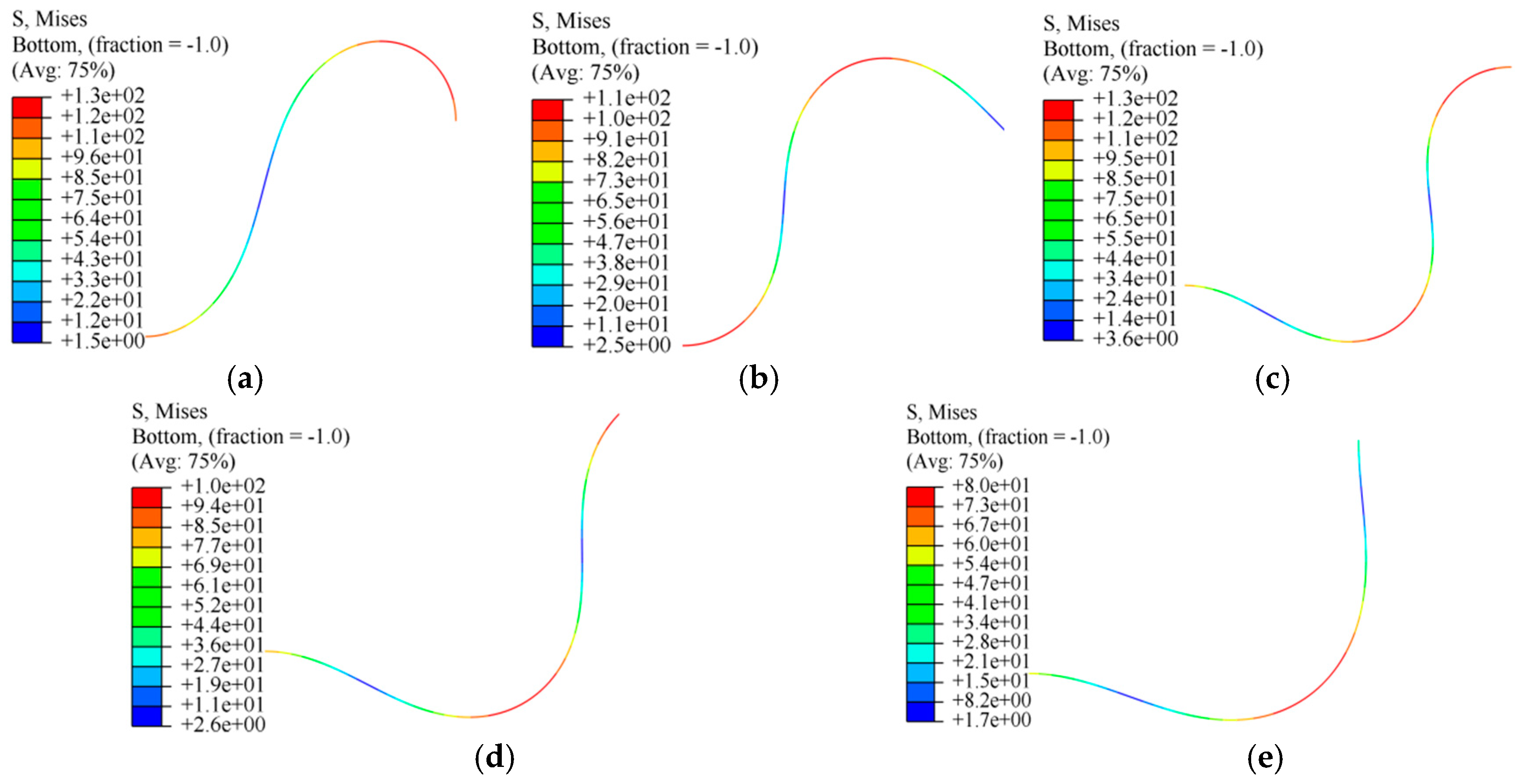
2.4. Bending Stress of Guidewire
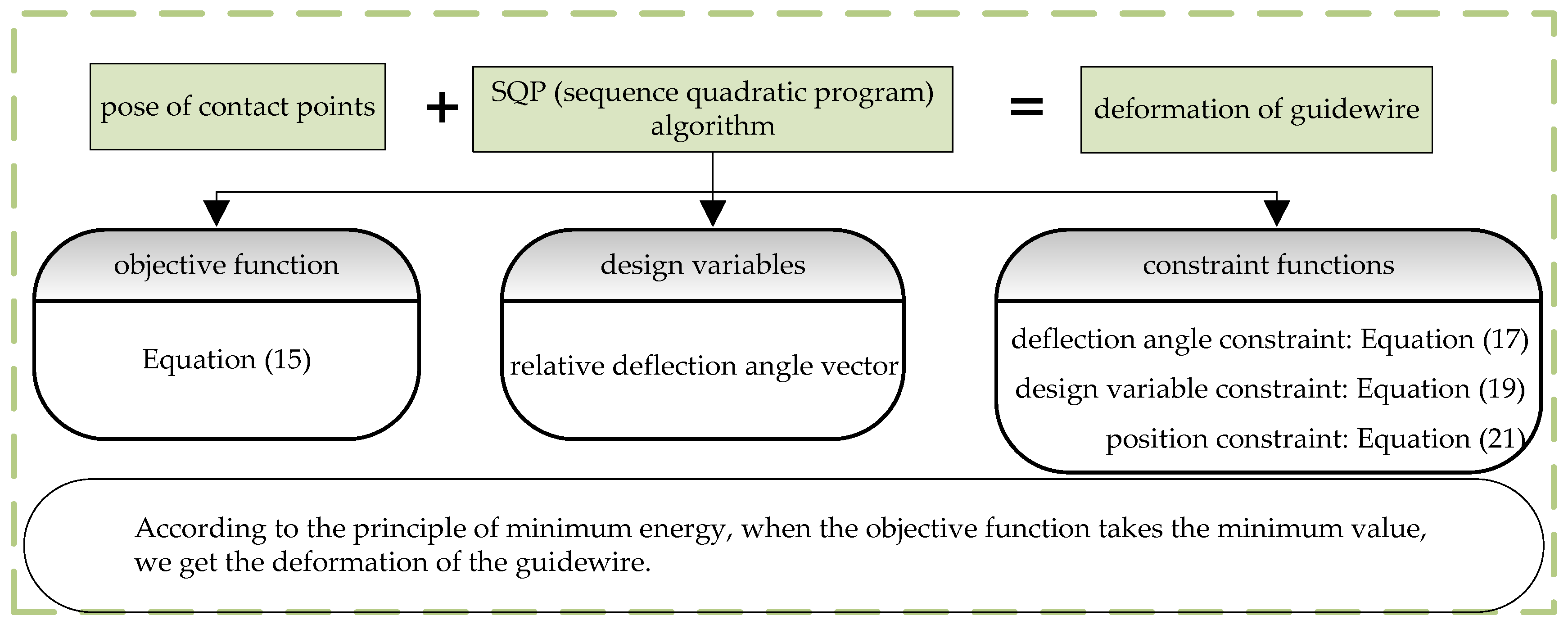
2.5. Summary of the Proposed Method
3. Results
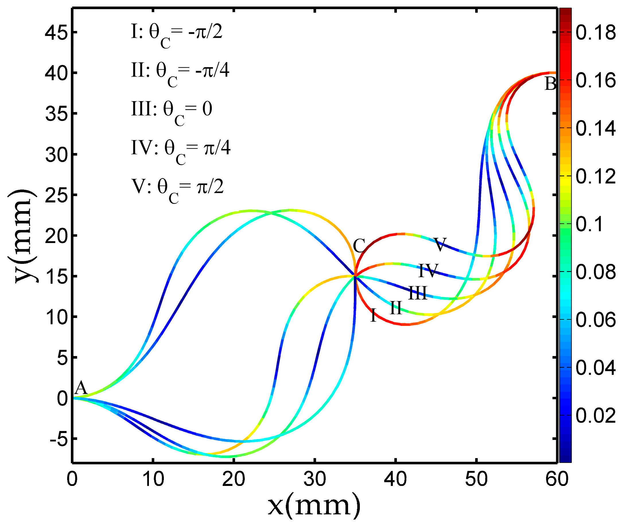
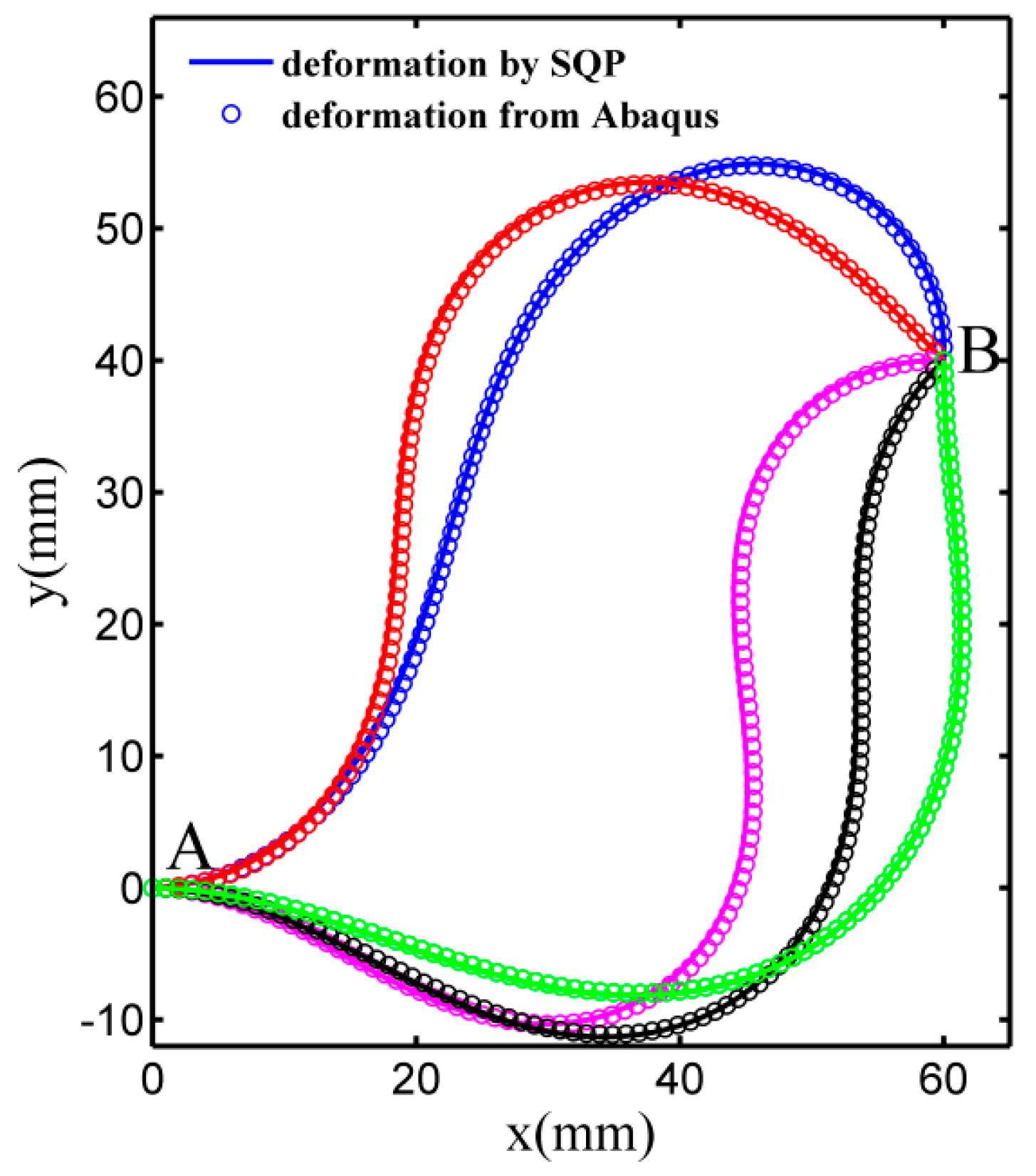
3.1. Deformation by SQP Algorithm
3.2. Deformation by ABAQUS Simulation
3.3. Discrete Density (n/L)
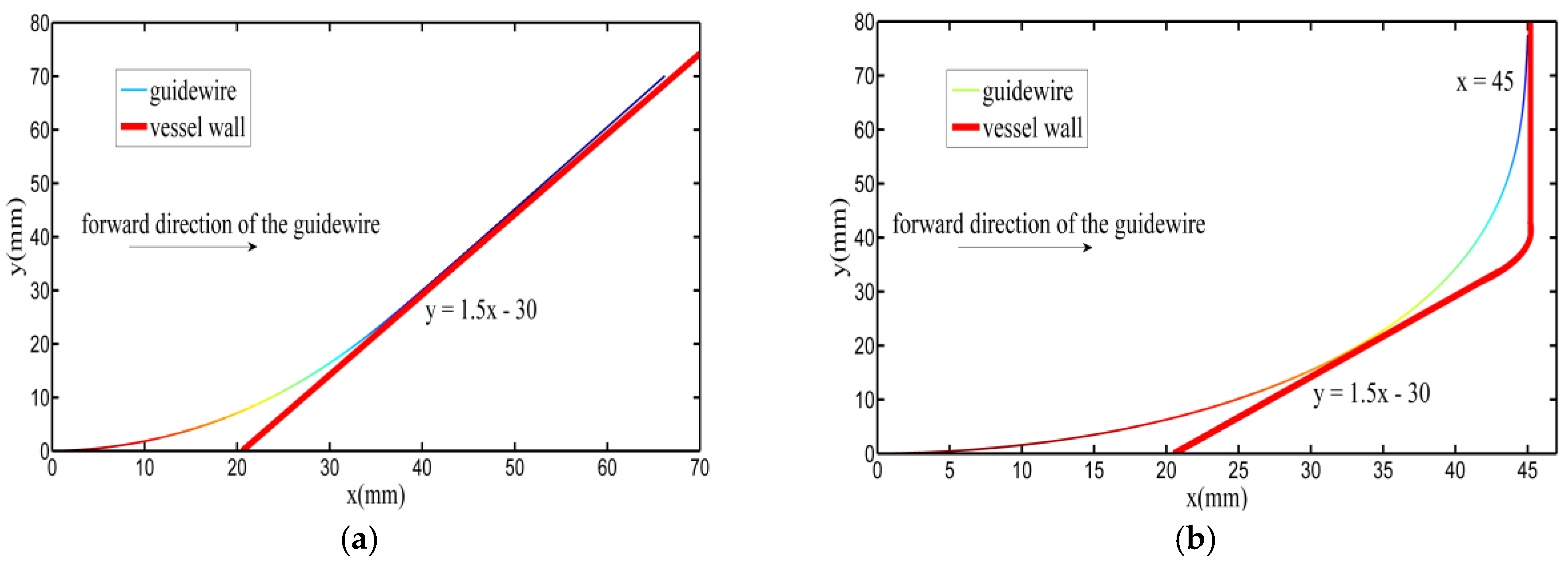
3.4. Experiments
4. Discussion
Author Contributions
Funding
Acknowledgments
Conflicts of Interest
References
- Dawson, S.; Gould, D.A. Procedural simulation’s developing role in medicine. Lancet 2007, 369, 1671–1673. [Google Scholar] [CrossRef]
- Ursino, M.; Tasto, J.L.; Nguyen, B.H.; Cunningham, R.; Merril, G.L. Cathsim: An intravascular catheterization simulator on a PC. Stud. Health Technol. Inform. 1999, 62, 360–366. [Google Scholar] [PubMed]
- 3D SYSTEMS. Available online: http://simbionix.com/simulators/angio-mentor/ (accessed on 12 October 2018).
- MENTICE. Available online: http://www.mentice.com/ (accessed on 12 October 2018).
- Alderliesten, T.; Konings, M.K.; Niessen, W.J. Simulation of minimally invasive vascular interventions for training purposes. Comput. Aided Surg. 2004, 9, 3–15. [Google Scholar] [CrossRef] [PubMed]
- Duratti, L.; Wang, F.; Samur, E.; Bleuler, H. A real-time simulator for interventional radiology. In Proceedings of the 2008 ACM Symposium on Virtual reality software and technology, Bordeaux, France, 27–29 October 2008; pp. 105–108. [Google Scholar]
- Gallagher, A.G.; Cates, C.U. Virtual reality training for the operating room and cardiac catheterisation laboratory. Lancet 2004, 364, 1538–1540. [Google Scholar] [CrossRef]
- Tang, W.; Lagadec, P.; Gould, D.; Wan, T.R.; Zhai, J.H.; How, T. A realistic elastic rod model for real-time simulation of minimally invasive vascular interventions. Vis. Comput. 2010, 26, 1157–1165. [Google Scholar] [CrossRef]
- Lenoira, J.; Cotin, S.; Duriez, C.; Neumann, P. Interactive physically-based simulation of catheter and guidewire. Comput. Graph. 2006, 30, 416–422. [Google Scholar] [CrossRef]
- Chiang, P.; Cai, Y.; Mak, K.H.; Soe, E.M.; Chui, C.K.; Zheng, J.M. A geometric approach to the modeling of the catheter–heart interaction for VR simulation of intra-cardiac intervention. Comput. Graph. 2011, 35, 1013–1022. [Google Scholar] [CrossRef]
- Ganji, Y.; Janabi-Sharifi, F. Catheter kinematics for intracardiac navigation. IEEE Trans. Biomed. Eng. 2009, 56, 621–632. [Google Scholar] [CrossRef] [PubMed]
- Nowinski, W.L.; Chui, C.K. Simulation of interventional neuroradiology procedures. In Proceedings of the IEEE Computer. Soc International Workshop on Medical Imaging and Augmented Reality, Hong Kong, China, 10–12 June 2001; pp. 87–94. [Google Scholar]
- Cotin, S.; Duriez, C.; Lenoir, J.; Neumann, P.; Dawson, S. New approaches to catheter navigation for interventional radiology simulation. In Proceedings of the Medical Image Computing and Computer-Assisted Intervention—MICCAI 2005, Palm Springs, CA, USA, 26–29 October 2005; pp. 534–542. [Google Scholar]
- Luboz, V.; Blazewski, R.; Gould, D.; Bello, F. Real-time guidewire simulation in complex vascular models. Vis. Comput. 2009, 25, 827–834. [Google Scholar] [CrossRef]
- Bergou, M.; Wardetzky, M.; Robinson, S.; Audoly, B.; Grinspun, E. Discrete elastic rods. ACM Trans. Graph. 2008, 27, 63. [Google Scholar] [CrossRef]
- Tang, W.; Wan, T.R.; Gould, D.A.; How, T.; John, N.W. A stable and real-time nonlinear elastic approach to simulating guidewire and catheter insertions based on cosserat rod. IEEE Trans. Biomed. Eng. 2012, 59, 2211–2218. [Google Scholar] [CrossRef] [PubMed]
- Dy, M.; Tagawa, K.; Tanaka, H.T.; Komori, M. Collision detection and modeling of rigid and deformable objects in laparoscopic simulator. In Proceedings of the Medical Imaging—Image-Guided Procedures, Robotic Interventions, and Modeling, Orlando, FL, USA, 22–24 February 2015. [Google Scholar]
- Johnsen, S.F.; Taylor, Z.A.; Han, L.; Hu, Y.; Clarkson, M.J.; Hawkes, D.J.; Ourselin, S. Detection and modelling of contacts in explicit finite-element simulation of soft tissue biomechanics. Int. J. Comput. Assist. Radiol. Surg. 2015, 10, 1873–1891. [Google Scholar] [CrossRef] [PubMed]
- Chang, J.; Wang, W.; Kim, M. Efficient collision detection using a dual OBB-sphere bounding volume hierarchy. Comput.-Aided Des. 2010, 42, 50–57. [Google Scholar] [CrossRef]
- Maciel, A.; Boulic, R.; Thalmann, D. Efficient collision detection within deforming spherical sliding contact. IEEE Trans. Vis. Comput. Graph. 2007, 13, 518–529. [Google Scholar] [CrossRef] [PubMed]
- Koh, S.K.; Liu, G. Optimal plane beams modelling elastic linear objects. Robotica 2010, 28, 135–148. [Google Scholar] [CrossRef]
- Hwang, Y.; Cha, S.L.; Kim, S.; Jin, S.S.; Jung, H.J. The multiple-update-infill sampling method using minimum energy design for sequential surrogate modeling. Appl. Sci. 2018, 8, 481. [Google Scholar] [CrossRef]
- Faroni, M.; Gorni, D.; Visioli, A. Energy Minimization in Time-Constrained Robotic Tasks via Sequential Quadratic Programming. In Proceedings of the 23rd IEEE International Conference on Emerging Technologies and Factory Automation (ETFA), Torino, Italy, 4–7 September 2018; pp. 699–705. [Google Scholar]
- Bonnans, J.F.; Gilbert, J.C.; Lemarechal, C.; Sagastizábal, C.A. Numerical optimization: Theoretical and practical aspects. IEEE Trans. Autom. Control 2003, 51, 541. [Google Scholar]
- Mittelstedt, M.; Hansenand, C.; Mertiny, P. Design and multi-objective optimization of fiber-reinforced polymer composite flywheel rotors. Appl. Sci. 2018, 8, 1256. [Google Scholar] [CrossRef]
- Tan, Q.F.; Wang, X.; Taghia, J.; Katupitiya, J. Force control of two-wheel-steer four-wheel-drive vehicles using model predictive control and sequential quadratic programming for improved path tracking. Int. J. Adv. Robot. Syst. 2017, 14, 1–15. [Google Scholar] [CrossRef]
- Carpinelli, G.; Mottola, F.; Proto, D.; Russo, A.; Varilone, P. A hybrid method for optimal siting and sizing of battery energy storage systems in unbalanced low Voltage microgrids. Appl. Sci. 2018, 8, 455. [Google Scholar] [CrossRef]


| Contact Point | Coordinate | Deflection Angle (Rad) | L(mm) | n |
|---|---|---|---|---|
| A | (0,0) | 0 | LAB = 100 | 100 |
| B | (60,40) | θB |
| Contact Point | Coordinate (mm) | Deflection Angle (Rad) | L(mm) | n |
|---|---|---|---|---|
| A | (0, 0) | 0 | LAB=100; LAC=50 | 100 |
| B | (60, 40) | 0 | ||
| C | (30, 20) | θC |
| Element | Cross Section | Length (mm) | Elastic Modulus (GPa) |
|---|---|---|---|
| beam | Circle, d = 0.78 mm | 100 | 3.56 |
| Poisson’s ratio | Constraint point A | Constarint point B | Mesh part |
| 0.3 | coordinate: (0,0) deflection angle: 0 | coordinate: (60,40) deflection angle: θB | 100 elements |
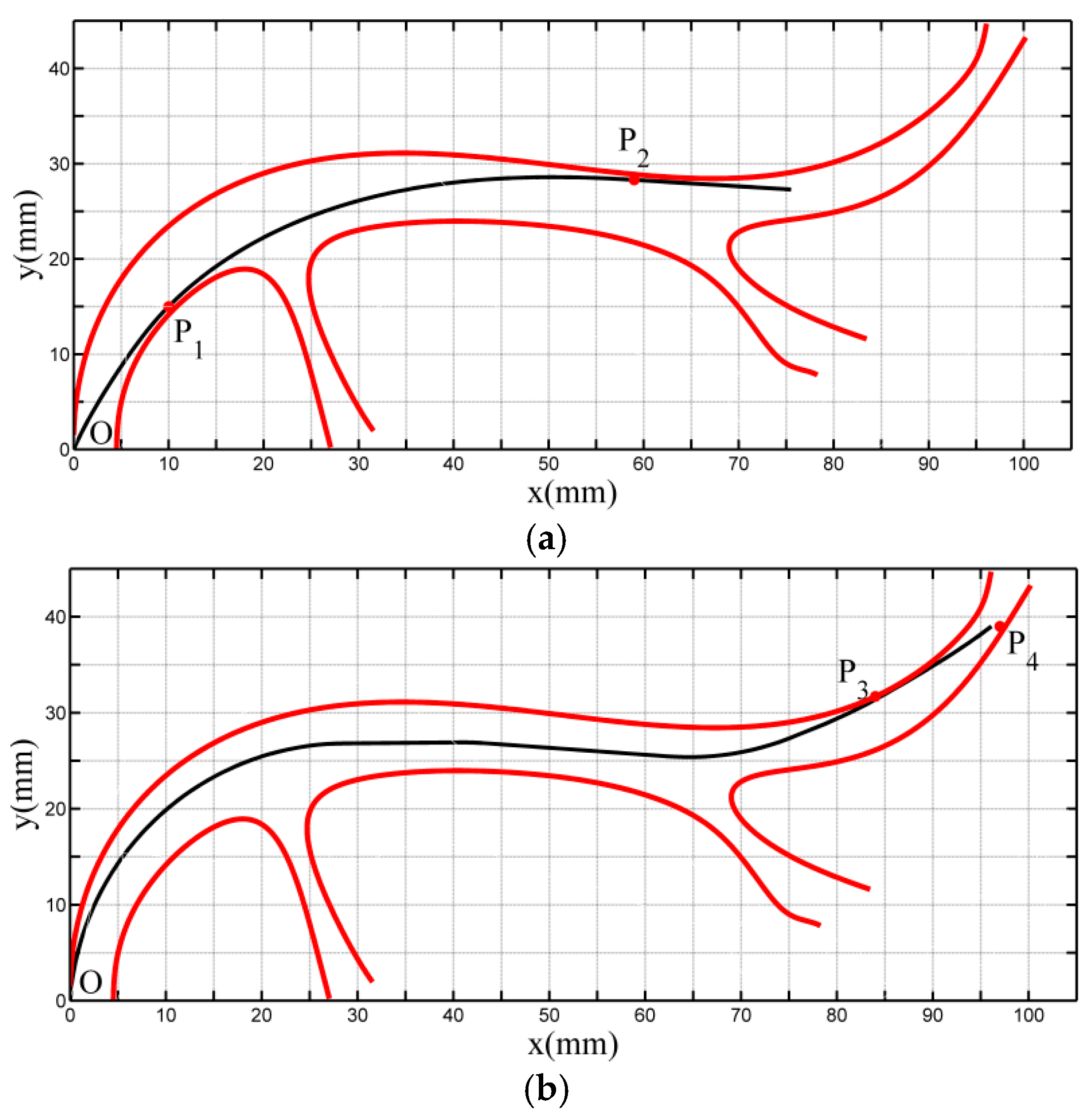
| Contact Points | Coordinate (mm) | Deflection Angle (Rad) | L (mm) | lin (mm) |
|---|---|---|---|---|
| O | (0,0) | 1.187 | - | 87 |
| P1 | (9.5,14.5) | 0.820 | ||
| P2 | (59, 28.3) | 0.061 |
| Contact Points | Coordinate (mm) | Deflection Angle (Rad) | L (mm) | lin (mm) |
|---|---|---|---|---|
| O | (0,0) | 1.518 | - | 112.5 |
| P3 | (80,28.5) | 0.244 | ||
| P4 | (98,42.5) | 0.644 |
© 2019 by the authors. Licensee MDPI, Basel, Switzerland. This article is an open access article distributed under the terms and conditions of the Creative Commons Attribution (CC BY) license (http://creativecommons.org/licenses/by/4.0/).
Share and Cite
Li, L.; Tang, Q.; Tian, Y.; Wang, W.; Chen, W.; Xi, F. Investigation of Guidewire Deformation in Blood Vessels Based on an SQP Algorithm. Appl. Sci. 2019, 9, 280. https://doi.org/10.3390/app9020280
Li L, Tang Q, Tian Y, Wang W, Chen W, Xi F. Investigation of Guidewire Deformation in Blood Vessels Based on an SQP Algorithm. Applied Sciences. 2019; 9(2):280. https://doi.org/10.3390/app9020280
Chicago/Turabian StyleLi, Long, Qijun Tang, Yingzhong Tian, Wenbin Wang, Wei Chen, and Fengfeng Xi. 2019. "Investigation of Guidewire Deformation in Blood Vessels Based on an SQP Algorithm" Applied Sciences 9, no. 2: 280. https://doi.org/10.3390/app9020280
APA StyleLi, L., Tang, Q., Tian, Y., Wang, W., Chen, W., & Xi, F. (2019). Investigation of Guidewire Deformation in Blood Vessels Based on an SQP Algorithm. Applied Sciences, 9(2), 280. https://doi.org/10.3390/app9020280