Predictions of Ship Extreme Hydroelastic Load Responses in Harsh Irregular Waves and Hull Girder Ultimate Strength Assessment


Abstract
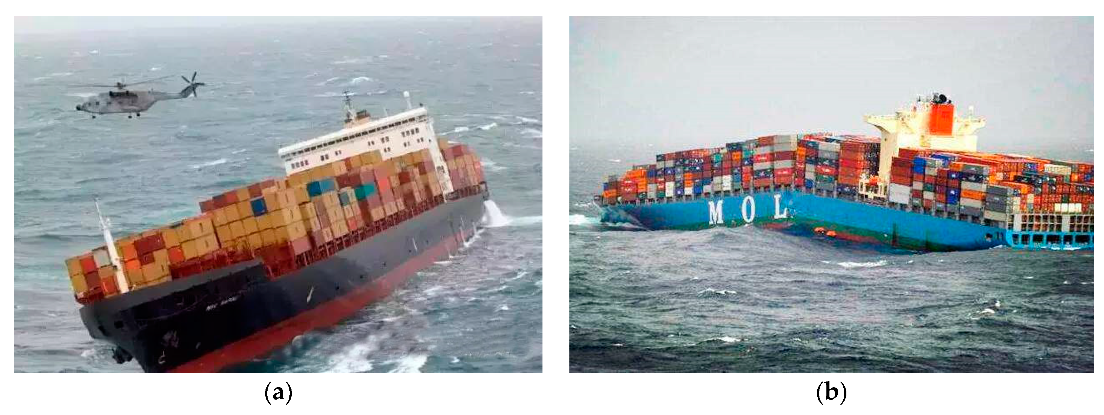
1. Introduction
2. Ship Hydroelasticity Theory in Irregular Waves
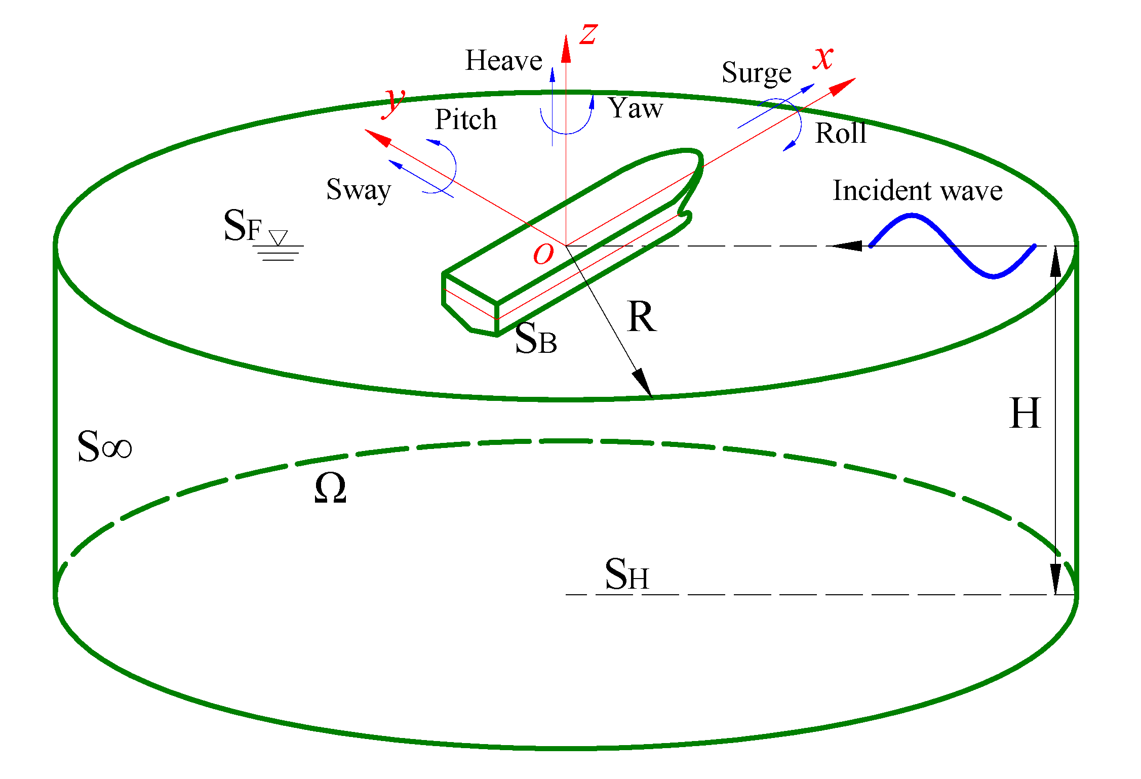
2.1. Potential Flow Theory in Ship Hydroelasticity
2.2. Solution of Hydroelastic Motion Equation
2.3. Prediction and Statistics of Extreme Values
3. Experimental Validation of the Hydroelasticity Theory
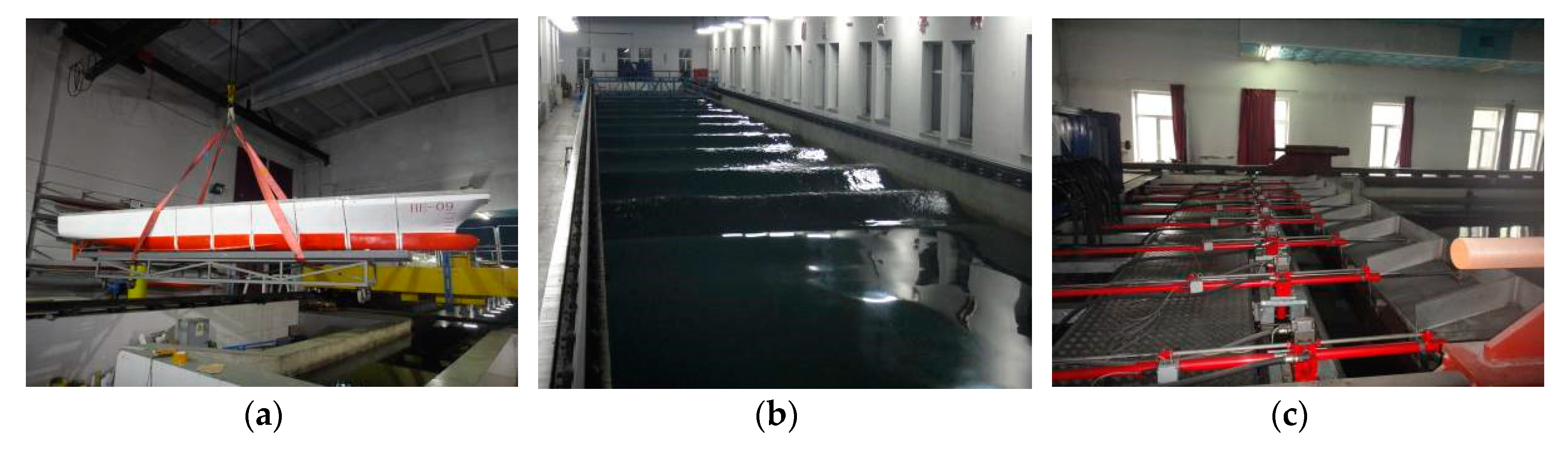
3.1. Experimental Setup
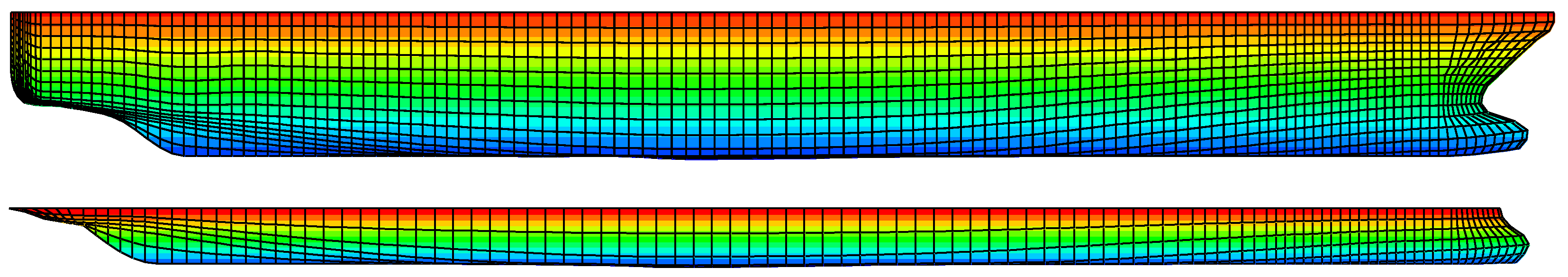
3.2. Numerical Setup
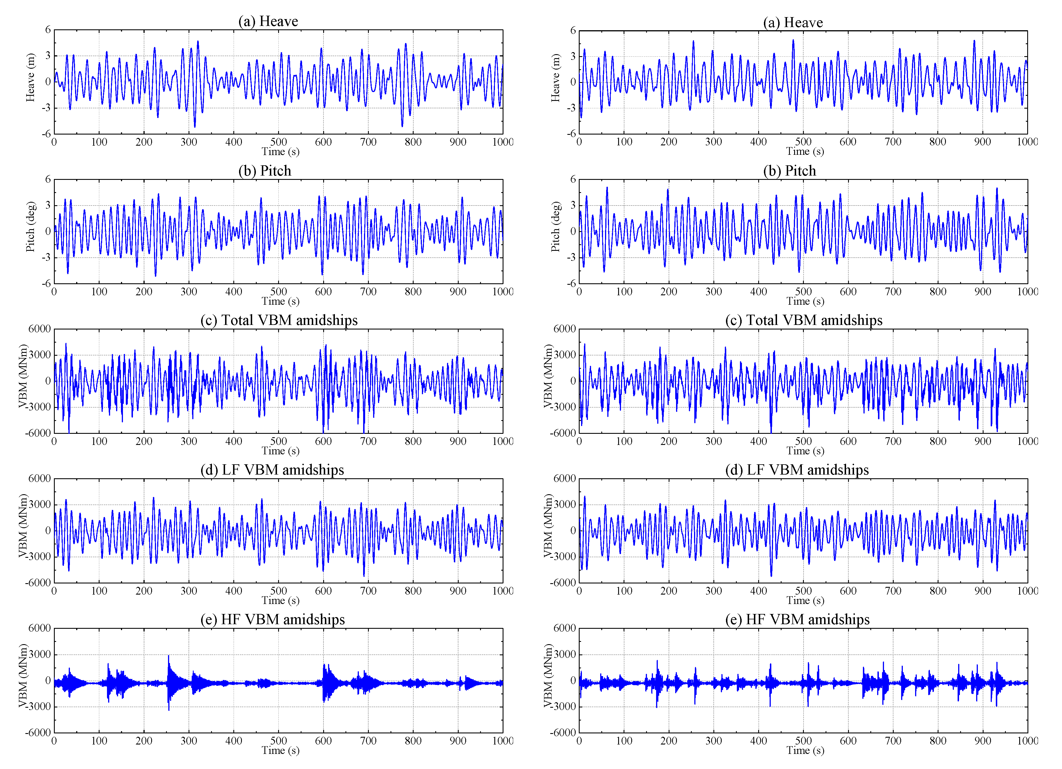
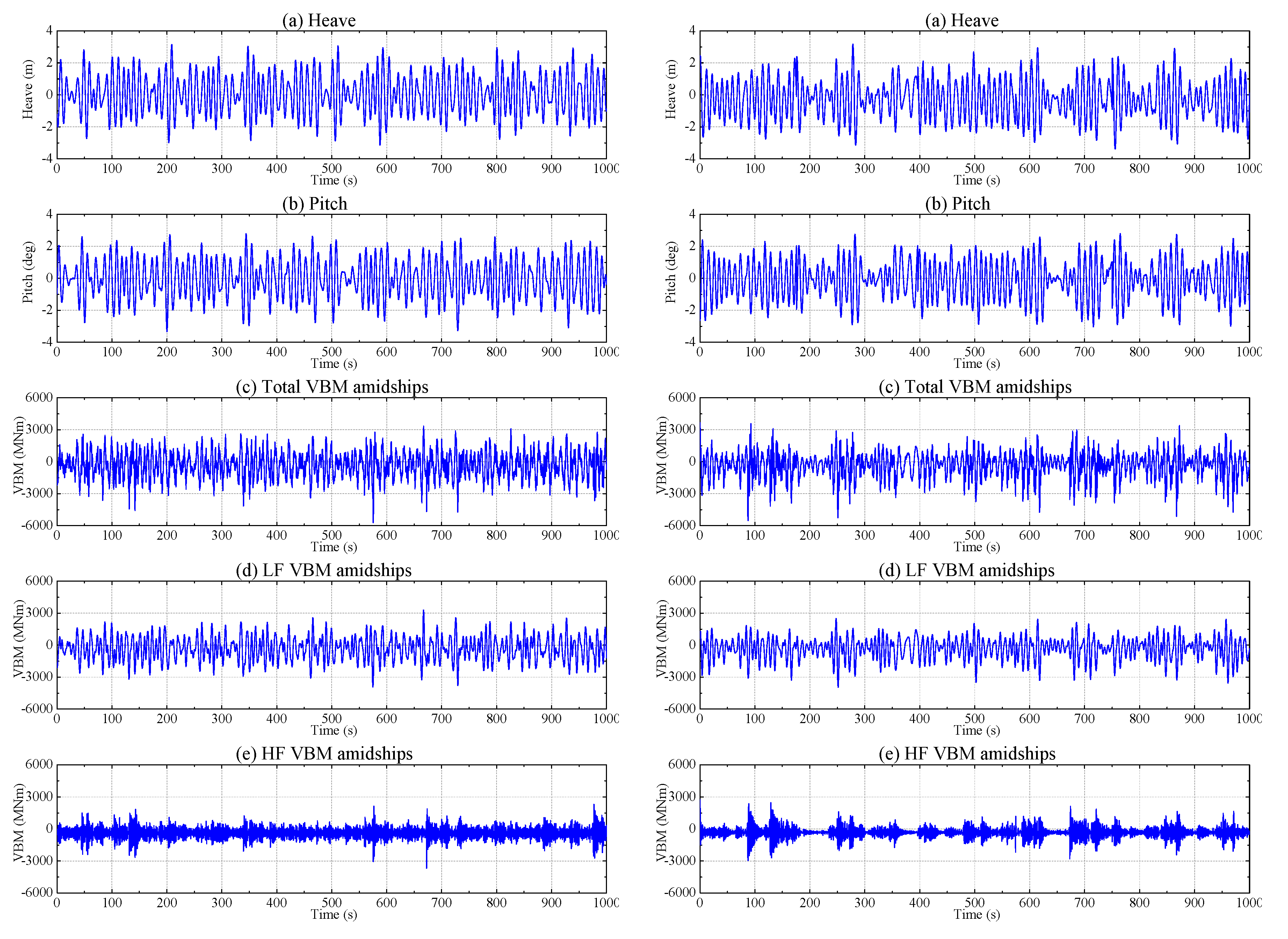
3.3. Comparison of Numerical and Experimental Time Series
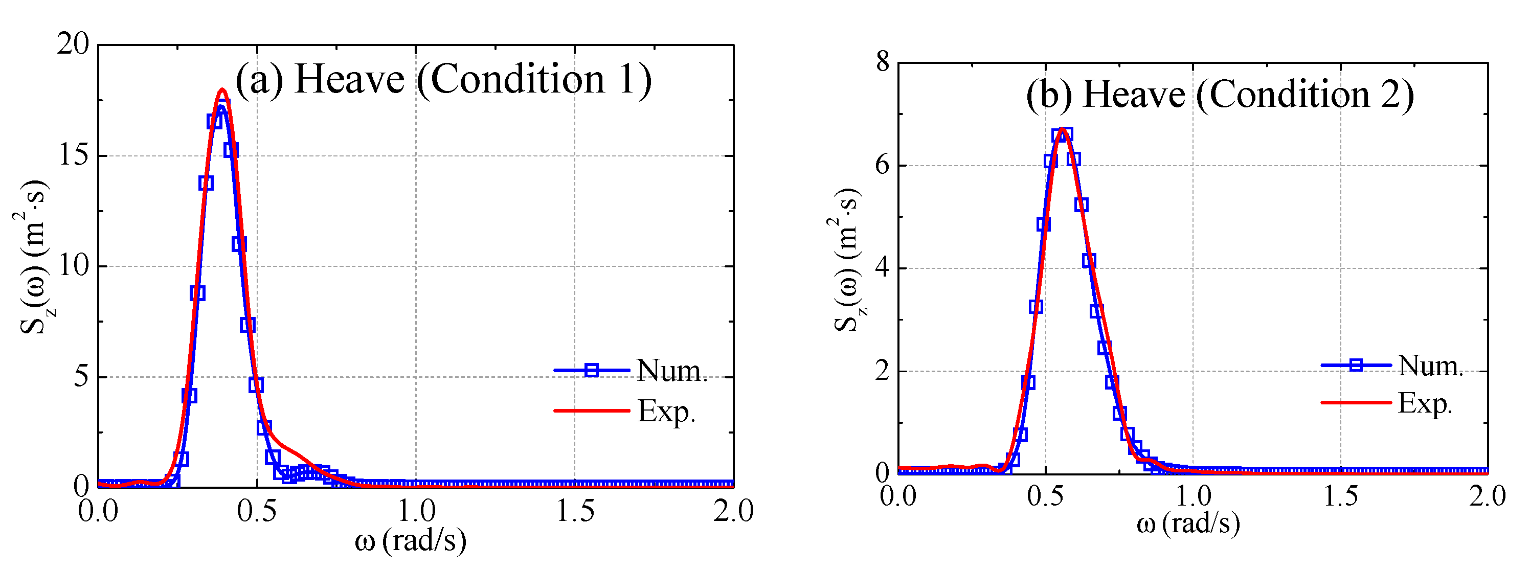
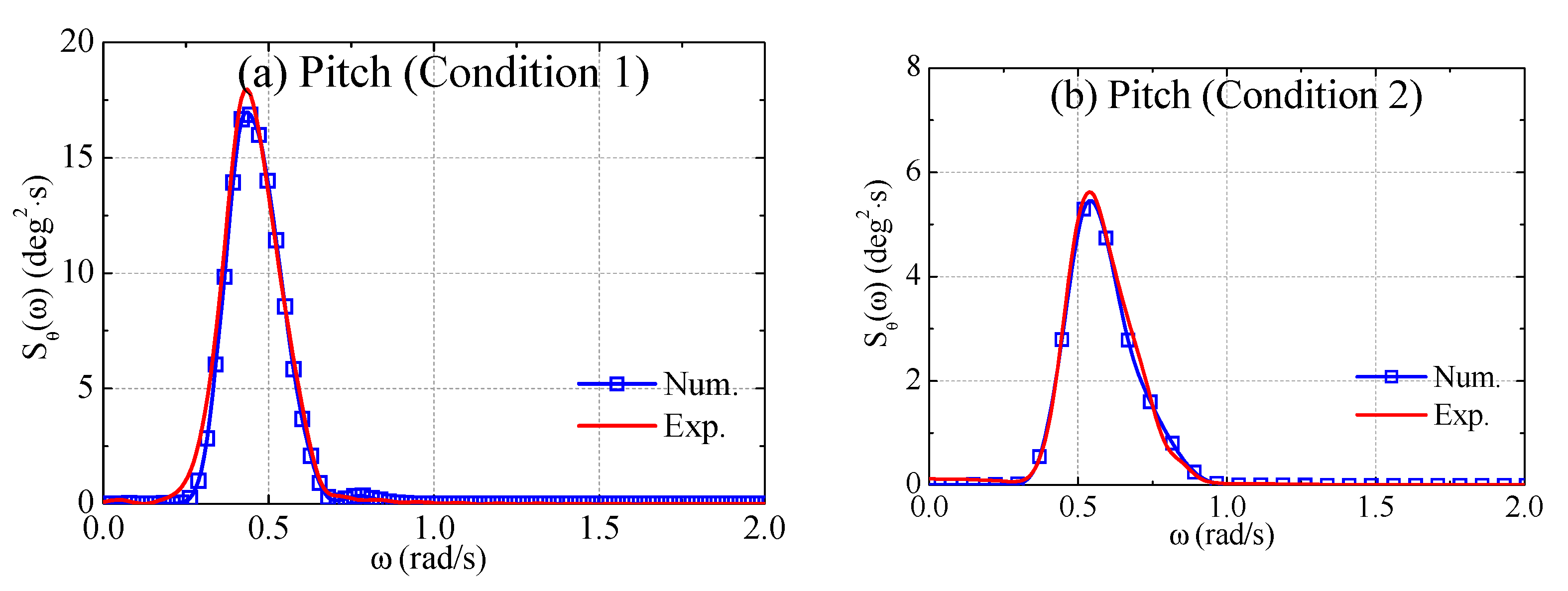
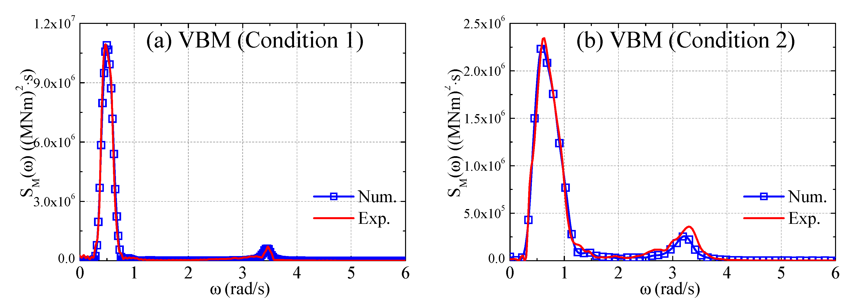
3.4. Comparison of Numerical and Experimental Spectra
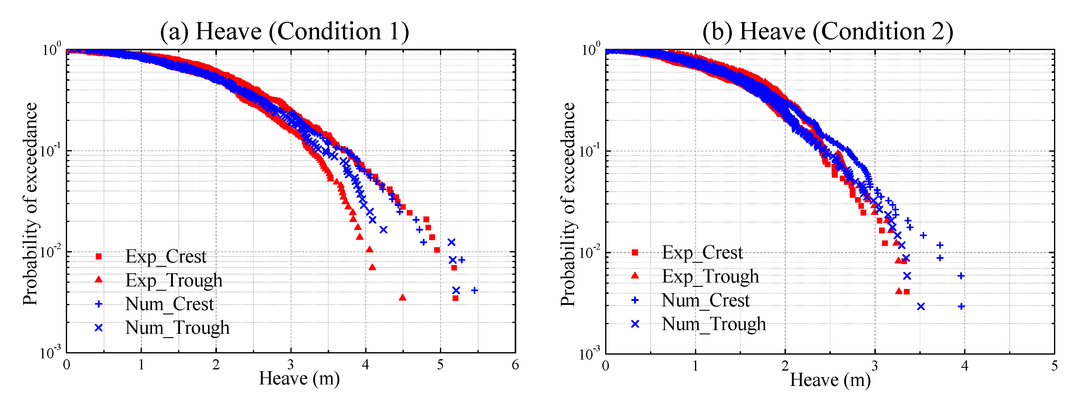
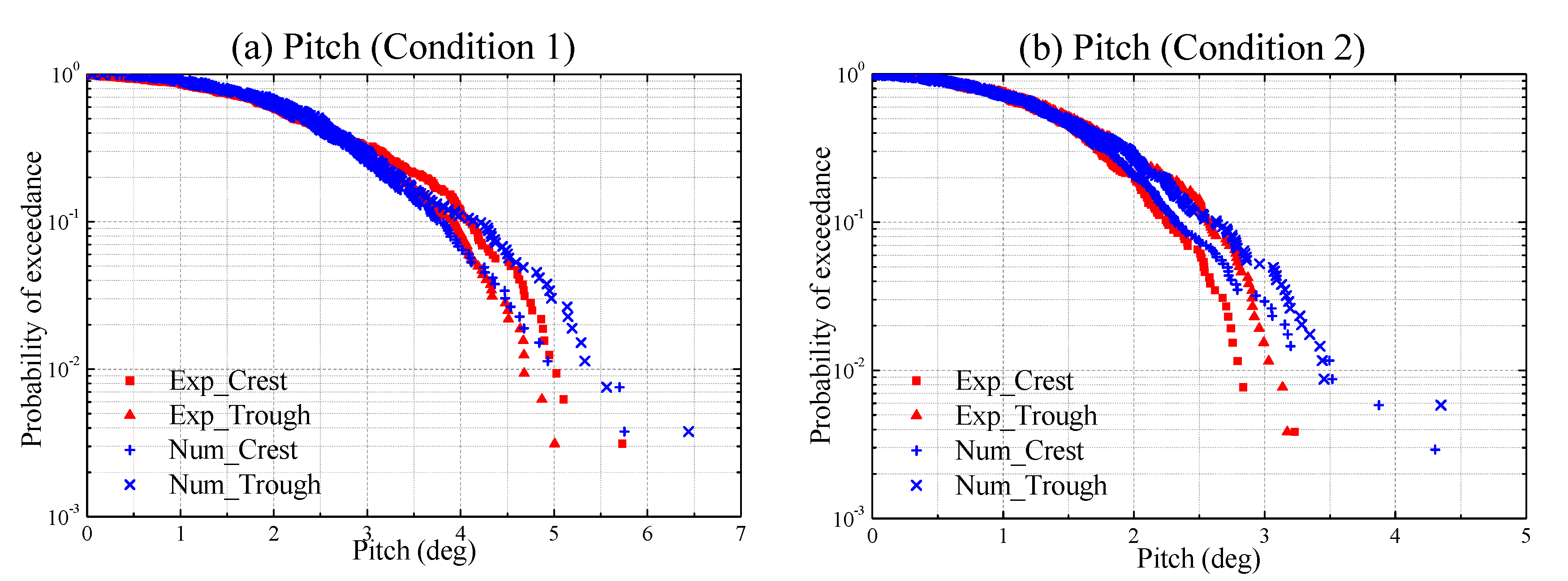
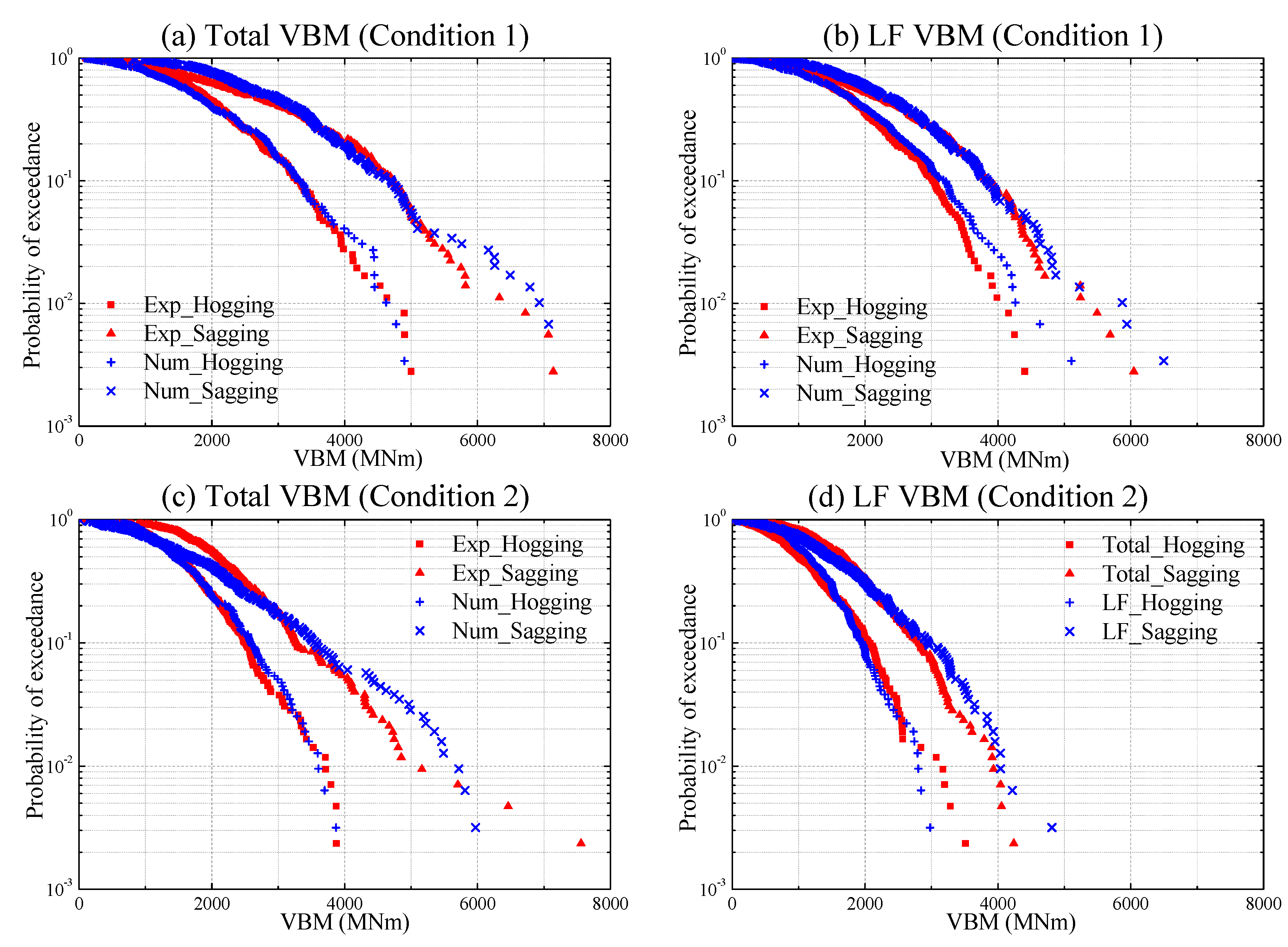
3.5. Probability of Exceedance of Numerical and Experimental Peaks
4. Statistical Analyses of Numerical Simulation Results
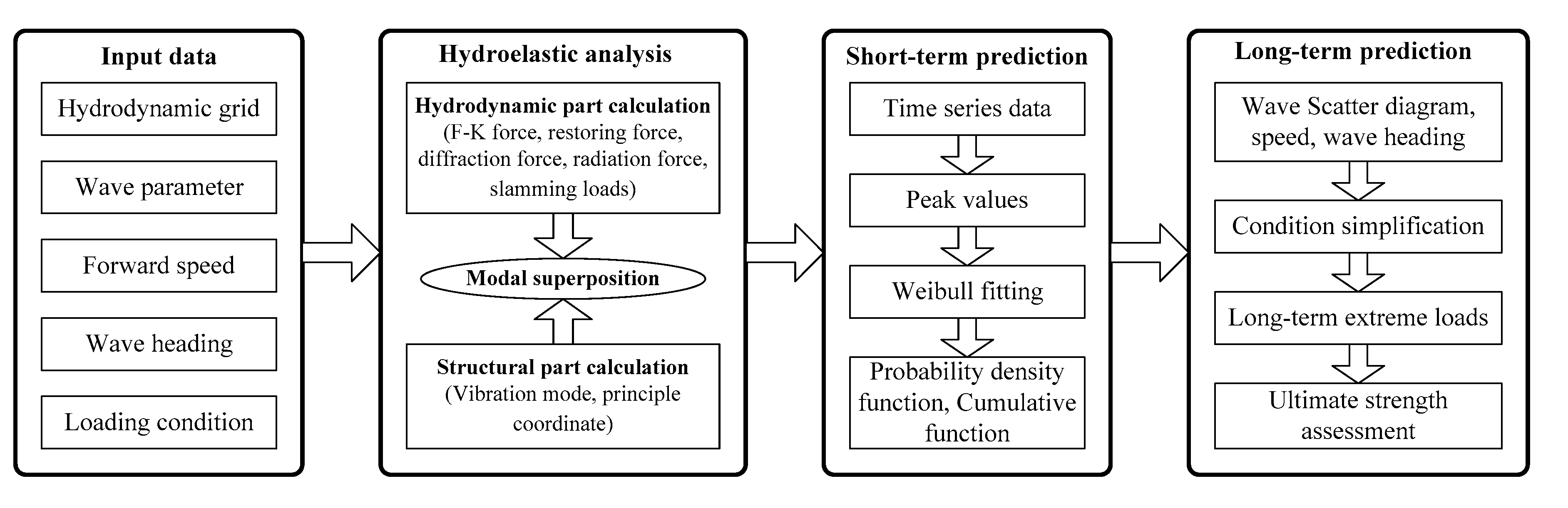
4.1. Calculation Method and Procedure
4.2. Simplification of Calculation Conditions for Long-Term Prediction
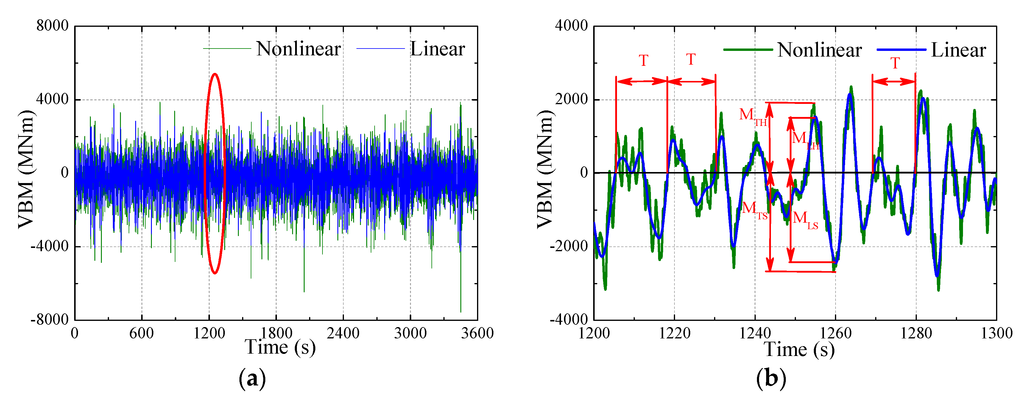
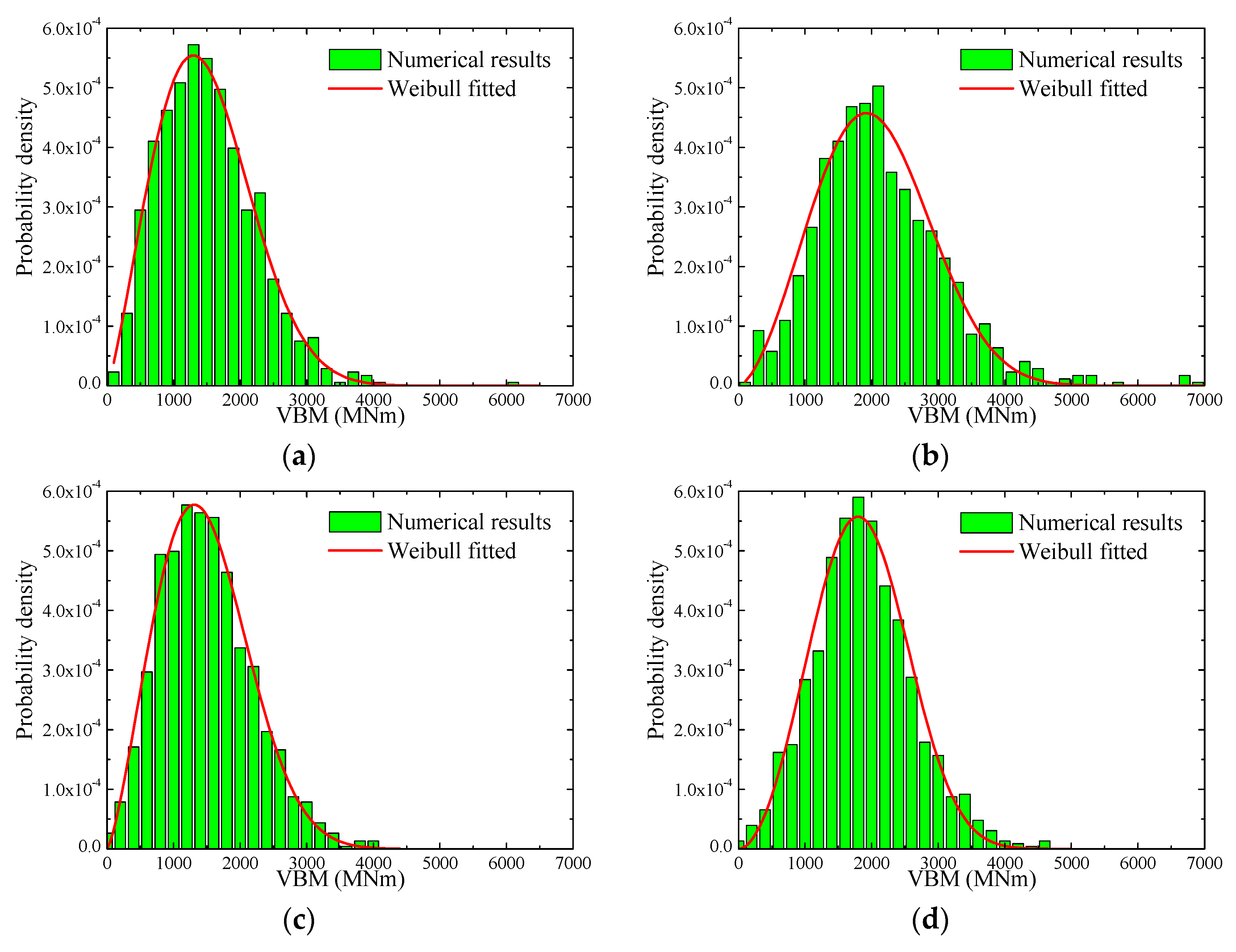
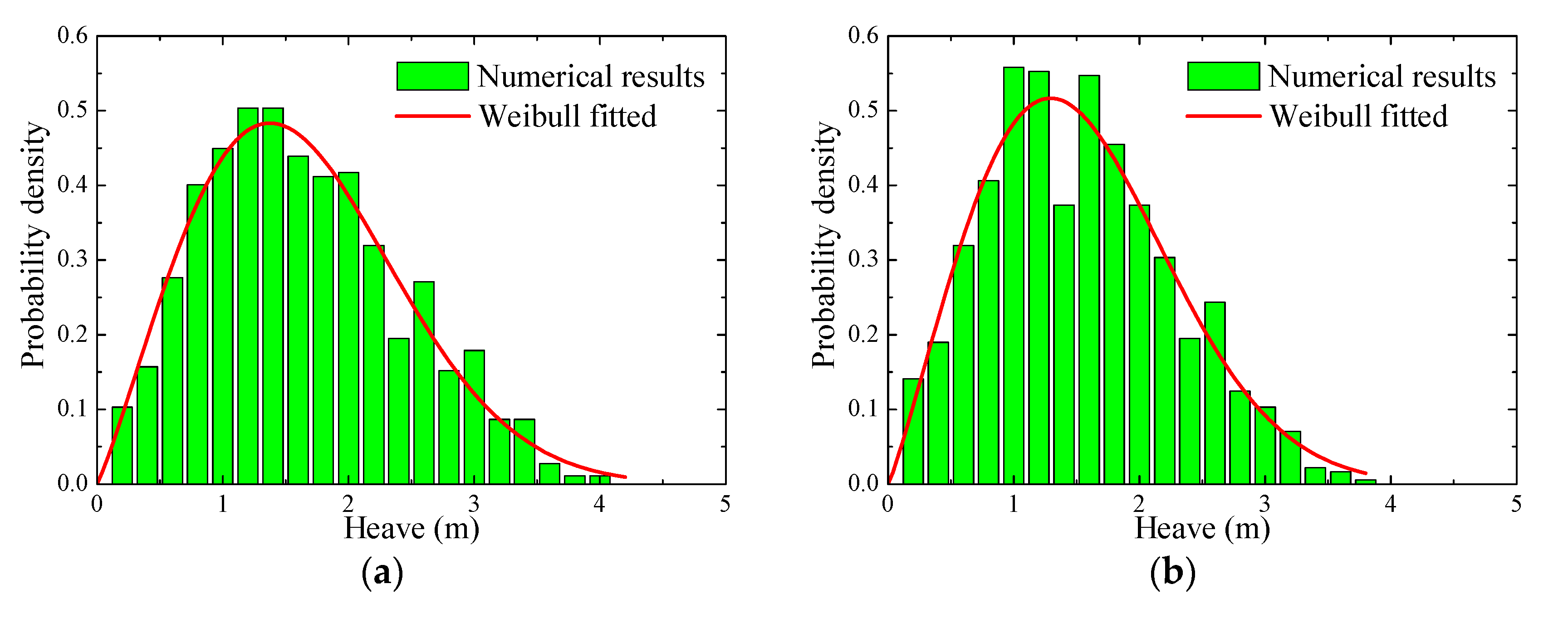
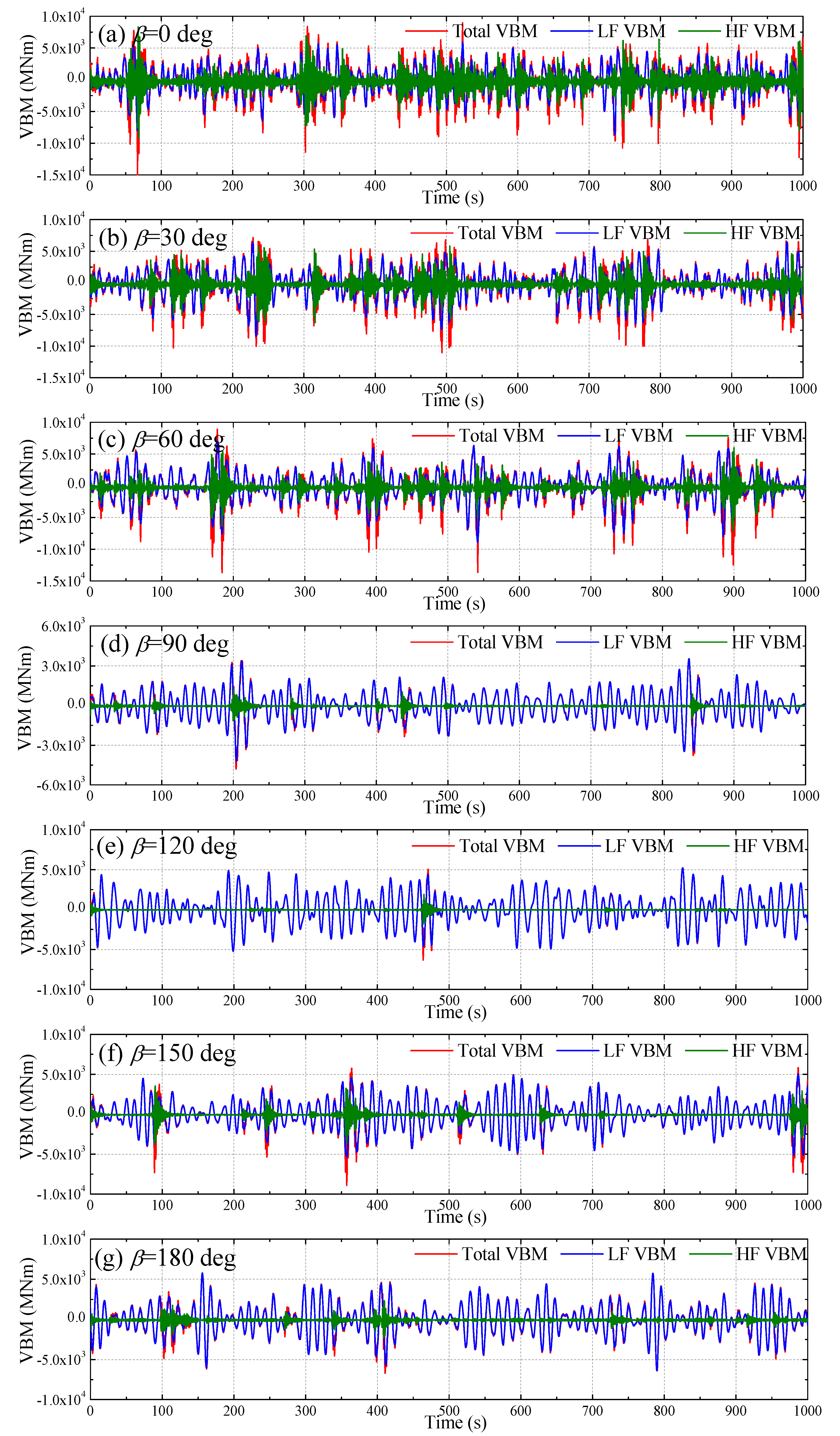
4.3. Short-Term Response Analyses
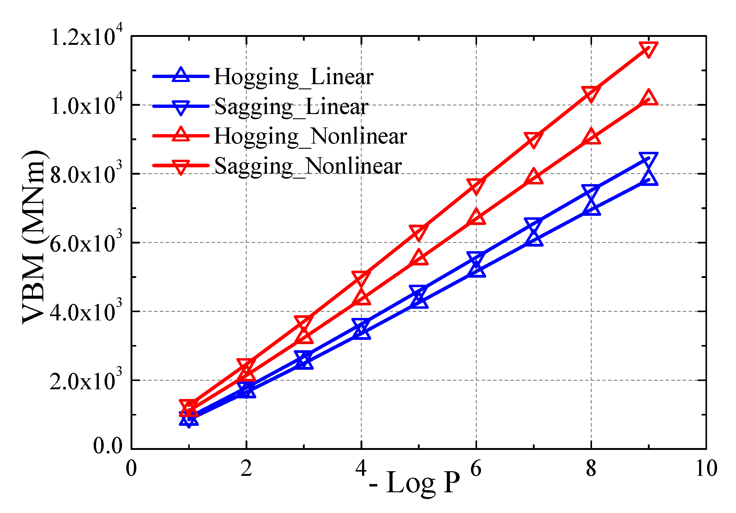
4.4. Long-Term Extreme Loads
5. Hull Girder Ultimate Strength Assessment
5.1. The Proposed Strength Check Formula
5.2. Determination of Design Loads by Rule Approach
- FS denotes distribution factor defined as follows: 0.2 at FP and AP points, 1 between 0.3 and 0.7 L, and liner interpolation at other intervals,
- C denotes wave coefficient calculated by C = 10.75 − (300 − L/100)1.5 for ships with a waterline length L between 90 and 300 m,
- L denotes ship waterline length, B denotes moulded breadth, CB denotes block coefficient,
- MWH and MWS denotes wave-induced VBM amidships in hogging and sagging, respectively. They are obtained as follows.
- FM denotes distribution factor defined as follows: 0 at FP and AP points, 1 between 0.4 and 0.65 L, and liner interpolation at other intervals,
- CA is coefficient obtained by CA = 7.1HA(1 + 1.26F)/L, where F denotes ship length Froude’s number,
- HA denotes wave parameter HA = CL/200 and without being taken greater than 0.8C.
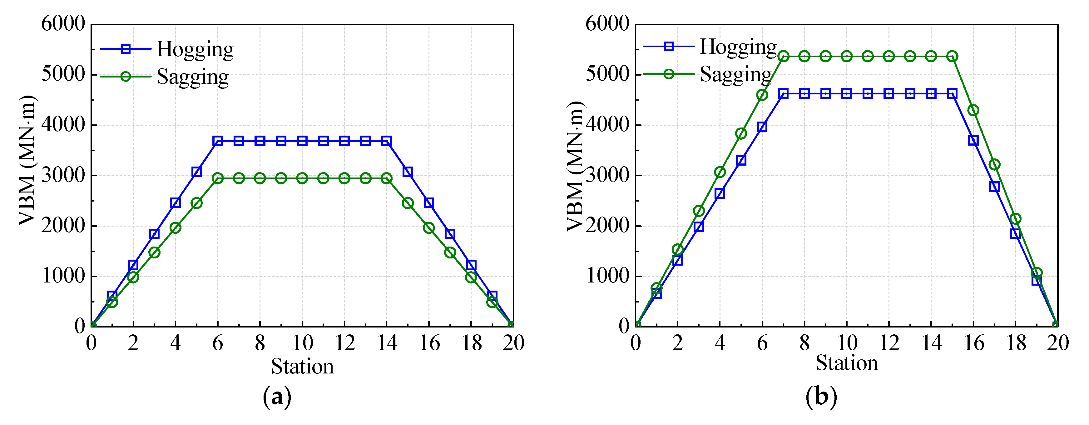
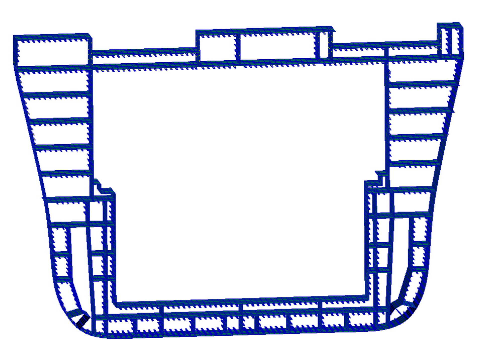
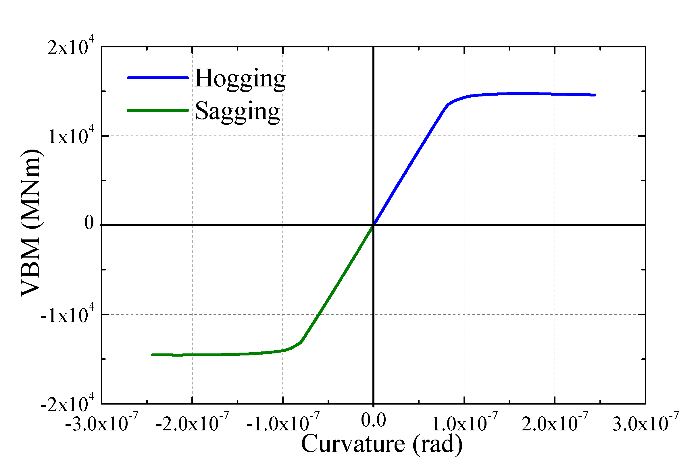
5.3. Ultimate Bearing Capacity Assessment
6. Conclusions
- (1)
- The developed time-domain hydroelastic theory, which combines 3D BEM and 1D beam model is reliable in the prediction of ship nonlinear motion and load responses and it has been well validated by comparison with the tank experimental results. Since the developed hydroelastic code runs much faster than the more complicated algorithm, which combines 3D BEM and 3D FEM, it is applicable for direct calculation of extreme wave loads and other nonlinear responses by performing long time numerical simulation.
- (2)
- The slamming induced whipping loads acting on ship when sailing in harsh waves and at high speed significantly increase the extreme loads for head or bow oblique wave conditions, while the whipping loads are very weak when ship sailing in beam or stern oblique waves. The long-term extreme VBM load predicted by nonlinear hydroelastic theory considering slamming effects is approximately 30% higher than that by linear hydroelastic theory. The simplification of simulation condition has ignorable small influence on the long-term extreme values.
- (3)
- Due to the fact that the effects of whipping loads on a hull girder’s ultimate strength is not well considered in the majority of the present Rule Book approaches, a simplified strength check formula, which includes the whipping load coefficient, is developed on the basis of the design wave loads by classification society Rule approach. The developed strength check formula is very useful for the hull girder ultimate strength assessment of a large flexible ship with a flare bow operating in harsh conditions.
Author Contributions
Funding
Conflicts of Interest
References
- Korvin-Kroukovsky, B.V.; Jacobs, W.R. Pitching and heaving motion of a ship in regular waves. Trans. Soc. Naval Archit. Mar. Eng. (SNAME) 1957, 65, 590–632. [Google Scholar]
- Salvesen, N.; Tuck, E.O.; Faltinsen, O.M. Ship motions and sea loads. Trans. Soc. Naval Archit. Mar. Eng. (SNAME) 1970, 78, 1–30. [Google Scholar]
- Sen, D. Time domain computation of large amplitude 3D ship motion with forward speed. Ocean Eng. 2002, 29, 973–1002. [Google Scholar] [CrossRef]
- Faltinsen, O.M.; Zhao, R. Numerical predictions of ship motions at high forward speed. Philos. Trans. Phys. Sci. Eng. 1991, 334, 241–252. [Google Scholar]
- Harding, R.D.; Hirdaris, S.E.; Miao, S.H.; Pittilo, M.; Temarel, P. Use of Hydroelasticity Analysis in Design. In Proceedings of the 4th International Conference on Hydroelasticity in Marine Technology, Wuxi, China, 10–14 September 2006; pp. 1–12. [Google Scholar]
- Heller, S.R.; Abramson, H.N. Hydroelasticity: A new naval science. J. Am. Soc. Naval Eng. 1959, 71, 205–209. [Google Scholar] [CrossRef]
- Lu, D.; Fu, S.; Zhang, X.; Guo, F.; Gao, Y. A method to estimate the hydroelastic behaviour of VLFS based on multi-rigid-body dynamics and beam bending. Ships Offshore Struct. 2016, 1–9. [Google Scholar] [CrossRef]
- Bishop, R.E.D.; Price, W.G. Hydroelasticity of Ships; Cambridge University Press: Cambridge, UK, 1979. [Google Scholar]
- Betts, C.V.; Bishop, R.E.D.; Price, W.G. The symmetric generalized fluid forces applied to a ship in a seaway. Trans. RINA 1977, 119, 265–278. [Google Scholar]
- Price, W.G.; Wu, Y.S. Hydroelasticity of marine structures. Theor. Appl. Mech. 1985, 316, 311–337. [Google Scholar]
- Hirdaris, S.E.; Temarel, P. Hydroelasticity of ships: Recent advances and future trends. Proc. Inst. Mech. Eng. Part M J. Eng. Marit. Environ. 2009, 223, 305–330. [Google Scholar] [CrossRef]
- Hirdaris, S.E.; Lee, Y.; Mortola, G.; Incecik, A.; Turan, O.; Hong, S.Y.; Temarel, P. The influence of nonlinearities on the symmetric hydrodynamic response of a 10,000 TEU Container ship. Ocean Eng. 2016, 111, 166–178. [Google Scholar] [CrossRef]
- Mortola, G.; Incecik, A.; Turan, O.; Hirdaris, S.E. Non linear analysis of ship motions and loads in large amplitude waves. Trans. Royal Inst. Naval Archit. Part A2 Int. J. Marit. Eng. 2011, 153, 81–87. [Google Scholar]
- Cheng, Y.; Okada, T.; Kobayakawa, H.; Miyashita, T.; Nagashima, T.; Neki, I. Simulation of whipping response of a large container ship fitted with a linear generator on board in irregular head seas. J. Mar. Sci. Technol. 2018, 23, 706–717. [Google Scholar] [CrossRef]
- Lee, Y.; White, N.; Wang, Z.; Zhang, S.; Hirdaris, S.E. Comparison of springing and whipping responses of model tests with predicted nonlinear hydroelastic analyses. Int. J. Offshore Polar Eng. 2012, 22, 1–8. [Google Scholar]
- Li, H.; Wang, D.; Liu, N.; Zhou, X.; Ong, M.C. Influence of linear springing on the fatigue damage of ultra large ore carriers. Appl. Sci. 2018, 8, 763. [Google Scholar] [CrossRef]
- Hong, S.Y.; Kim, B.W. Experimental investigations of higher-order springing and whipping-WILS project. Int. J. Nav. Archit. Ocean Eng. 2014, 6, 1160–1181. [Google Scholar] [CrossRef]
- Kim, J.H.; Kim, Y.; Korobkin, A. Comparison of fully coupled hydroelastic computation and segmented model test results for slamming and whipping loads. Int. J. Nav. Archit. Ocean Eng. 2014, 6, 1064–1081. [Google Scholar] [CrossRef]
- Southall, N.; Choi, S.; Lee, Y.; Hong, C.; Hirdaris, S.; White, N. Impact Analysis Using CFD—A Comparative Study. In Proceedings of the Twenty-fifth (2015) International Ocean and Polar Engineering Conference, Kona, HI, USA, 21–26 June 2015; pp. 692–698. [Google Scholar]
- Xu, J.; Sun, Y.; Li, Z.; Zhang, X.; Lu, D. Analysis of the hydroelastic performance of very large floating structures based on multimodules beam theory. Math. Probl. Eng. 2017, 1–14. [Google Scholar] [CrossRef]
- Chen, Z.Y.; Jiao, J.L.; Li, H. Time-domain numerical and segmented ship model experimental analyses of hydroelastic responses of a large container ship in oblique regular waves. Appl. Ocean Res. 2017, 67, 78–93. [Google Scholar] [CrossRef]
- Kara, F. Time domain prediction of hydroelasticity of floating bodies. Appl. Ocean Res. 2015, 51, 1–13. [Google Scholar] [CrossRef]
- Rajendran, S.; Vasquez, G.; Soares, C.G. Effect of bow flare on the vertical ship responses in abnormal waves and extreme seas. Ocean Eng. 2016, 124, 49–436. [Google Scholar] [CrossRef]
- Wang, S.; Soares, C.G. Experimental and numerical study of the slamming load on the bow of a chemical tanker in irregular waves. Ocean Eng. 2016, 111, 369–383. [Google Scholar] [CrossRef]
- Kim, J.H.; Kim, Y. Prediction of extreme loads on ultra-large containerships with structural hydroelasticity. J. Mar. Sci. Technol. 2018, 23, 253–266. [Google Scholar] [CrossRef]
- Jiao, J.; Zhao, Y.; Ai, Y.; Chen, C.; Fan, T. Theoretical and Experimental Study on Nonlinear Hydroelastic Responses and Slamming Loads of Ship Advancing in Regular Waves. Shock Vib. 2018, 2018, 1–26. [Google Scholar] [CrossRef]
- Soares, C.G.; Fonseca, N.; Pascoal, R. Long term prediction of non-linear vertical bending moments on a fast monohull. Appl. Ocean Res. 2004, 26, 288–297. [Google Scholar] [CrossRef]
- Baarholm, G.S.; Moan, T. Estimation of nonlinear long-term extremes of hull girder loads in ships. Mar. Struct. 2000, 13, 495–516. [Google Scholar] [CrossRef]
- Wu, M.K.; Hermundstad, O.A. Time-domain simulation of wave-induced nonlinear motions and loads and its applications in ship design. Mar. Struct. 2002, 15, 561–597. [Google Scholar] [CrossRef]
- International Association of Classification Societies (IACS). Unified Requirements S11; Longitudinal Strength Standard; IACS: London, UK, 2015. [Google Scholar]
- Mohammed, E.A.; Benson, S.D.; Hirdaris, S.E.; Dow, R.S. Design safety margin of a 10,000 TEU container ship through ultimate hull girder load combination analysis. Mar. Struct. 2016, 46, 78–101. [Google Scholar] [CrossRef]
- China Classification Society (CCS). Guidelines for Influence of Springing and Whipping Loads on Hull Girder Fatigue Strength; CCS: Beijing, China, 2015. [Google Scholar]
- Bureau Veritas (BV). Rules for the Classification of Military Ships; Part B-Hull and Stability; BV: Paris, France, 2003. [Google Scholar]


| Item | Symbol | Full Scale | Small Model |
|---|---|---|---|
| Scale | λ | 1:1 | 1:50 |
| Overall length (m) | LOA | 312 | 6.24 |
| Waterline length (m) | L | 292 | 5.84 |
| Moulded breadth (m) | B | 39.5 | 0.79 |
| Depth (m) | D | 25.5 | 0.51 |
| Draft (m) | T | 10.1 | 0.202 |
| Block coefficient | CB | 0.616 | 0.616 |
| Displacement (t) | Δ | 71,875 | 0.575 |
| Hs/Tz | 1.5 | 2.5 | 3.5 | 4.5 | 5.5 | 6.5 | 7.5 | 8.5 | 9.5 | 10.5 | 11.5 | 12.5 | 13.5 | 14.5 | 15.5 | 16.5 | 17.5 | 18.5 | Sum |
|---|---|---|---|---|---|---|---|---|---|---|---|---|---|---|---|---|---|---|---|
| 0.5 | 1.3 | 133 | 865 | 1186 | 634 | 186 | 36.9 | 5.6 | 0.7 | 0.1 | 3050 | ||||||||
| 1.5 | 29.3 | 986 | 4976 | 7738 | 5569 | 2375 | 703 | 160 | 30.5 | 5.1 | 0.8 | 0.1 | 22,575 | ||||||
| 2.5 | 2.2 | 197 | 2158 | 6230 | 7449 | 4860 | 2066 | 644 | 160 | 33.7 | 6.3 | 1.1 | 0.2 | 23,810 | |||||
| 3.5 | 0.2 | 34.9 | 695 | 3226 | 5675 | 5099 | 2838 | 1114 | 377 | 84.3 | 18.2 | 3.5 | 0.6 | 0.1 | 19,128 | ||||
| 4.5 | 6 | 196 | 1354 | 3288 | 3857 | 2685 | 1275 | 455 | 130 | 31.9 | 6.9 | 1.3 | 0.2 | 13,289 | |||||
| 5.5 | 1 | 51 | 498 | 1602 | 2372 | 2008 | 1126 | 463 | 150 | 41 | 9.7 | 2.1 | 0.4 | 0.1 | 8328 | ||||
| 6.5 | 0.2 | 12.6 | 167 | 690 | 1257 | 1268 | 825 | 386 | 140 | 42.2 | 10.9 | 2.5 | 0.5 | 0.1 | 4806 | ||||
| 7.5 | 3 | 52.1 | 270 | 594 | 703 | 524 | 276 | 111 | 36.7 | 10.2 | 2.5 | 0.6 | 0.1 | 2586 | |||||
| 8.5 | Percentage | 0.7 | 15.4 | 97.9 | 255 | 350 | 296 | 174 | 77.6 | 27.7 | 8.4 | 2.2 | 0.5 | 0.1 | 1309 | ||||
| 9.5 | 0–100 | 0.2 | 4.3 | 33.2 | 101 | 159 | 152 | 99.2 | 48.3 | 18.7 | 6.1 | 1.7 | 0.4 | 0.1 | 626 | ||||
| 10.5 | 100–500 | 1.2 | 10.7 | 37.9 | 67.5 | 71.7 | 51.5 | 27.3 | 11.4 | 4 | 1.2 | 0.3 | 0.1 | 285 | |||||
| 11.5 | 500–1000 | 0.3 | 3.3 | 13.3 | 26.6 | 31.4 | 24.7 | 14.2 | 6.4 | 2.4 | 0.7 | 0.2 | 0.1 | 124 | |||||
| 12.5 | 1000–2000 | 0.1 | 1 | 4.4 | 9.9 | 12.8 | 11 | 6.8 | 3.3 | 1.3 | 0.4 | 0.1 | 51 | ||||||
| 13.5 | 2000–3000 | 0.3 | 1.4 | 3.5 | 5 | 4.6 | 3.1 | 1.6 | 0.7 | 0.2 | 0.1 | 21 | |||||||
| 14.5 | 3000–5000 | 0.1 | 0.4 | 1.2 | 1.8 | 1.8 | 1.3 | 0.7 | 0.3 | 0.1 | 8 | ||||||||
| 15.5 | 5000–7000 | 0.1 | 0.4 | 0.6 | 0.7 | 0.5 | 0.3 | 0.1 | 0.1 | 3 | |||||||||
| 16.5 | 7000- | 0.1 | 0.2 | 0.2 | 0.2 | 0.1 | 0.1 | 1 | |||||||||||
| Sum | 0 | 0 | 1 | 165 | 2091 | 9280 | 19,922 | 24,879 | 20,870 | 12,898 | 6245 | 2479 | 837 | 247 | 66 | 16 | 3 | 1 | 100,000 |
| H1/3 (m) | U (knot) |
|---|---|
| 0 < H1/3 ≤ 6 | Vs |
| 6 < H1/3 ≤ 9 | 75%Vs |
| 9 < H1/3 ≤ 12 | 50%Vs |
| 12 < H1/3 | 25%Vs (≥5) |
| Item | Full Conditions | Simplified Conditions | Error | |
|---|---|---|---|---|
| Nonlinear results (MNm) | Hogging | 9036 | 9030 | 0.07% |
| Sagging | 10382 | 10370 | 0.12% | |
| Linear results (MNm) | Hogging | 6971 | 6959 | 0.17% |
| Sagging | 7533 | 7516 | 0.23% | |
| Ratio coefficient | Hogging | 1.296 | 1.298 | 0.15% |
| Sagging | 1.378 | 1.380 | 0.15% | |
| Item | Symbol | Hoging | Saging |
|---|---|---|---|
| Calm water VBM | MS (MNm) | 3688 | 2948 |
| Wave-induced VBM | MW (MNm) | 4627 | 5366 |
| Extreme VBM by nonlinear direct calculation | Mwhip (MNm) | 9036 | 10,382 |
| Extreme VBM by linear direct calculation | Mwave (MNm) | 6971 | 7533 |
| Correction factor due to whipping loads | fwhip | 1.30 | 1.38 |
| Safety factor of MS | γS | 1.00 | 1.00 |
| Safety factor of MW | γW | 1.10 | 1.10 |
| Safety factor of MU | γR | 1.15 | 1.15 |
| Safety factor of material uncertainty | γM | 1.02 | 1.02 |
| Safety factor of condition simplification | Cun | 1.01 | 1.01 |
| Ultimate bearing capacity VBM | MU (MNm) | 14,713 | 14,550 |
| Strength check by Rule approach | MTotal (MNm) | 10,305 | 11,094 |
| Failure ratio | 82% | 88% | |
| Safety satisfy? | Yes | Yes | |
| Strength check by direct calculation | MTotal (MNm) | 9036 | 10,382 |
| Failure ratio | 72% | 83% | |
| Safety satisfy? | Yes | Yes |
© 2019 by the authors. Licensee MDPI, Basel, Switzerland. This article is an open access article distributed under the terms and conditions of the Creative Commons Attribution (CC BY) license (http://creativecommons.org/licenses/by/4.0/).
Share and Cite
Jiao, J.; Jiang, Y.; Zhang, H.; Li, C.; Chen, C. Predictions of Ship Extreme Hydroelastic Load Responses in Harsh Irregular Waves and Hull Girder Ultimate Strength Assessment. Appl. Sci. 2019, 9, 240. https://doi.org/10.3390/app9020240
Jiao J, Jiang Y, Zhang H, Li C, Chen C. Predictions of Ship Extreme Hydroelastic Load Responses in Harsh Irregular Waves and Hull Girder Ultimate Strength Assessment. Applied Sciences. 2019; 9(2):240. https://doi.org/10.3390/app9020240
Chicago/Turabian StyleJiao, Jialong, Yong Jiang, Hao Zhang, Chengjun Li, and Chaohe Chen. 2019. "Predictions of Ship Extreme Hydroelastic Load Responses in Harsh Irregular Waves and Hull Girder Ultimate Strength Assessment" Applied Sciences 9, no. 2: 240. https://doi.org/10.3390/app9020240
APA StyleJiao, J., Jiang, Y., Zhang, H., Li, C., & Chen, C. (2019). Predictions of Ship Extreme Hydroelastic Load Responses in Harsh Irregular Waves and Hull Girder Ultimate Strength Assessment. Applied Sciences, 9(2), 240. https://doi.org/10.3390/app9020240