Article

Building an Effective Intrusion Detection System Using the Modified Density Peak Clustering Algorithm and Deep Belief Networks

1
School of Cyberspace Security, Beijing University of Posts and Telecommunications, Beijing 100876, China
2
College of Information Science and Engineering, Xinjiang University, Urumqi 830046, China
3
Guizhou Provincial Key Laboratory of Public Big Data, Guizhou University, Guiyang 550025, China
*
Author to whom correspondence should be addressed.
Appl. Sci. 2019, 9(2), 238; https://doi.org/10.3390/app9020238
Submission received: 11 December 2018 / Revised: 1 January 2019 / Accepted: 4 January 2019 / Published: 10 January 2019
(This article belongs to the Section Computing and Artificial Intelligence)

Abstract

:

Featured Application

The model proposed in this paper can be deployed to the enterprise gateway, dynamically monitor network activities, and connect with the firewall to protect the company network from attacks. It can be deployed in cloud computing environment or in software-defined networks to monitor network behavior and alerts in real time.

Abstract

Machine learning plays an important role in building intrusion detection systems. However, with the increase of data capacity and data dimension, the ability of shallow machine learning is becoming more limited. In this paper, we propose a fuzzy aggregation approach using the modified density peak clustering algorithm (MDPCA) and deep belief networks (DBNs). To reduce the size of the training set and the imbalance of the samples, MDPCA is used to divide the training set into several subsets with similar sets of attributes. Each subset is used to train its own sub-DBNs classifier. These sub-DBN classifiers can learn and explore high-level abstract features, automatically reduce data dimensions, and perform classification well. According to the nearest neighbor criterion, the fuzzy membership weights of each test sample in each sub-DBNs classifier are calculated. The output of all sub-DBNs classifiers is aggregated based on fuzzy membership weights. Experimental results on the NSL-KDD and UNSW-NB15 datasets show that our proposed model has higher overall accuracy, recall, precision and F1-score than other well-known classification methods. Furthermore, the proposed model achieves better performance in terms of accuracy, detection rate and false positive rate compared to the state-of-the-art intrusion detection methods.

Graphical Abstract

1. Introduction

Today, with the rapid growth and the wide application of the Internet and Intranet, computer networks have brought great convenience to people’s life and work. However, at the same time, they also brought a lot of security problems, such as various types of viruses, vulnerabilities and attacks, which cause heavy losses. How can necessary protection and security be provided for computer networks, and their integrity and availability be maintained? This question has become a hot issue in research. Intrusion Detection System (IDS) is an important security device or software application in a network environment. It is widely used to monitor network activities and detect whether the system is subjected to network attacks such as DoS (Denial of Service) attacks. According to the analysis method and detection principle, IDS can be anomaly-based detection or misuse-based detection [1,2]. In this work, we focus on misuse-based IDS.
In recent years, many researchers have introduced more and more innovative techniques to detect intrusions, such as machine learning, data mining and swarm intelligence. In the literature, these techniques are divided into three categories. The first category is the anomaly detection methods, which require normal datasets to train the classifier and determine whether the new data sample is in conformity with the model. Examples of these methods include the cluster algorithm [3], SOM (Self-Organizing Map) [4] and GMM (Gaussian Mixture Model) [5]. The second category uses an individual machine learning algorithm to solve intrusion detection problems, such as KNN (K-Nearest Neighbor) [6,7], SVM (Support Vector Machines) [8], ANN (Artificial Neural Network) [9], DT (Decision Tree) [10], etc. The last category uses various ensemble and hybrid techniques, combined with various machine learning techniques to improve detection performance. These methods include Bagging, Boosting, Stacking, and combined classifier methods [11]. RF (Random Forest) [12] is an ensemble learning method based on bagging, which builds a classification model from a multitude of decision trees. AdaBoost (Adaptive Boosting) [13] is a popular boosting method that has the ability to adapt to errors associated with weak hypotheses. The idea of Stacking is that the output of a set of classifiers is used as the input of another classifier [14].
In 2006, Hinton proposed Deep Belief Networks (DBNs) [15,16], which made deep learning the meteoric rise in the field of machine learning. In recent years, deep learning has become a hot research topic, and has achieved great success in extracting high-level latent features from data samples. Deep learning can reconstruct the approximate compression of the original features and has been successfully used in many applications such as speech recognition, natural language processing, image processing, network security detection [17,
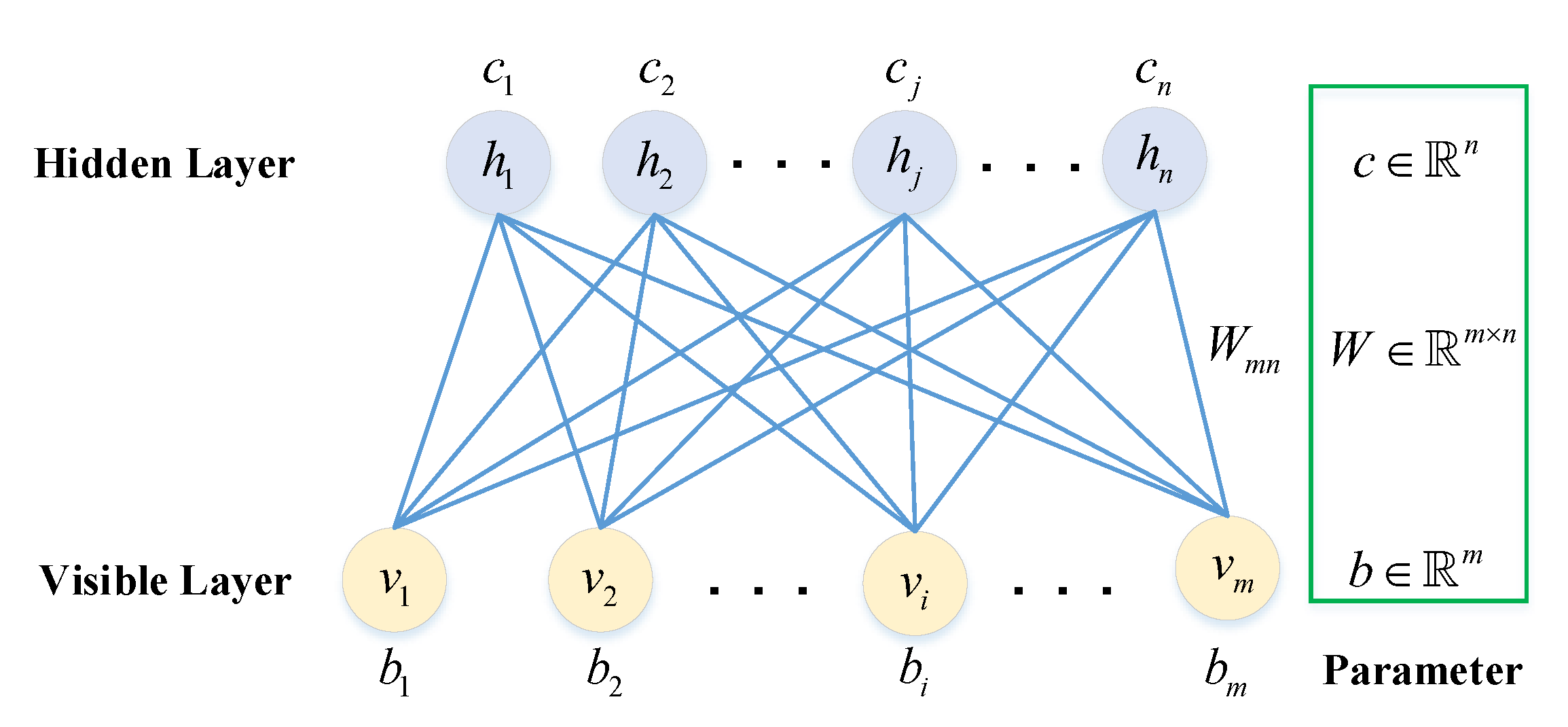
18], and so on. DBNs are probabilistic generative neural network composed by several layers of RBMs (Restricted Boltzmann Machines) and a single layer of BP (Back Propagation) neural network. RBMs are used to initialize the neural network through a pre-training process, which can make the initialization parameters of neural network closer to the global optimal value, and make the network training easier to achieve global optimization. Huda et al. [19] used optimal deep belief networks to detect malware behaviors.
However, there are still many problems with intrusion detection systems. First, different types of network traffic in a real network environment are imbalanced, and network intrusion records are less than normal records. As a result, unbalanced network traffic greatly compromises the detection performance of most classifiers. The classifier is biased towards the more frequently occurring records, which reduces the detection rate of small attack records such as U2R and R2L records. Second, due to the high dimensionality of network data, the feature selection methods in many intrusion models are first considered as one of the preprocessing steps [20], such as PCA (Principal Component Analysis) and chi-square feature selection. However, these feature selection methods rely heavily on manual feature extraction, mainly through experience and luck, and these algorithms are not effective enough. Third, because of the large amount of network traffic and complex structure, the traditional classifier algorithm cannot achieve higher attack detection rate with lower false positive rate. Fourth, the network operating environment and structure in the real world are changing, for example, the popularity of the Internet of Things and the widespread use of cloud services, as well as various new attacks are emerging. Many unknown attacks do not appear in the training dataset. For example, for the NSL-KDD [21,22] dataset, 16.6% of the attack samples in the test dataset did not appear in the training dataset [23]. As a result, all traditional intrusion detection methods usually perform poorly.
Taking into account the above factors, we propose a novel fuzzy aggregation method called MDPCA-DBN, which combines the modified density peak clustering algorithm (MDPCA) and the deep belief networks (DBNs). The MDPCA divides the original training dataset into several smaller subsets according to the feature similarity of the training samples. These subsets are used to train their respective sub-DBNs classifiers. These sub-DBNs can automatically extract high-level abstract features from the training samples and reduce the dimensions of network traffic data without heuristic rules and manual experience. DBNs integrate feature extraction and classification into a system that extracts high-level features by identifying network traffic and classifies them based on labeled samples. In the test phase, the fuzzy membership weight of each test sample in each sub-DBNs classifier is calculated based on the nearest neighbor criteria of the training sample cluster. Then, each test sample is tested in each trained sub-DBNs classifier. Finally, the output of all sub-DBNs classifiers is aggregated based on the fuzzy membership weights.
The key contributions of this paper are as follows. First, we improve the Euclidean distance calculation method of the density peak clustering algorithm (DPCA) [24], and use the kernel function to project the original features into the high-dimensional kernel space to better cluster the complex nonlinear inseparable network traffic data. Second, we use MDPCA to extract similar features of complex network data and divide the network dataset into several subsets with different clusters. Compared with the original dataset, these subsets reduce the imbalance of multi-class network data and improve the detection rate of the minority classes. Third, we use DBNs to automatically extract high-level features from massive and complex network traffic data and perform classification. DBNs with several hidden layers initialize network parameters through greedy layer-by-layer unsupervised learning algorithms, and adjust network weights by backpropagation and fine-tuning to better solve the classification problem of complex, large-scale and nonlinear network traffic data. The deep generation model can obtain a better attack classification than the shallow machine learning algorithm, and can solve many nonlinear problems of complex and massive data. Finally, we have evaluated the proposed method on the NSL-KDD [21,22] and UNSW-NB15 [25,26,27] datasets. Experimental results show that, compared with the well-known classification algorithms, the proposed method achieved better performance in terms of accuracy, detection rate and false positive rate.
The rest of this paper is organized as follows. Section 2 introduces intrusion detection related works based on RBM and deep learning. In Section 3, we detail the MDPCA and DBNs algorithms. Section 4 presents the proposed hybrid model for intrusion detection and describes how the model works. Section 5 demonstrates the experimental details and results. Finally, we draw some conclusions and suggest the further work in Section 6.

2. Related Works

As far as we know, there are no reports on DPCA and DBN hybrid methods for intrusion detection, although related works to DPCA have been done in other areas. Cha et al. [28] employed the DPCA algorithm for structural damage detection. Li et al. [29] proposed a hybrid model combining the core ideas of KNN and DPCA for intrusion detection. The model uses the idea of density and the process of the k-nearest neighbors to detect attacks. Ma et al. [30] presented a hybrid method combining spectral clustering and deep neural networks, named SCDNN. SCDNN uses spectral clustering to divide the training set and test set into several subsets, and then input them into the deep neural network for intrusion detection. They reported an overall accuracy of 72.64% on the NSL-KDD dataset. The clustering algorithm and classifier of SCDNN are spectral clustering (not DPCA) and DNN (not DBN), respectively. Moreover, the output of SCDNN on the test set is only a simple summary, without any integration principle. This is completely different from our proposed method.
The deep learning method integrates high-level feature extraction and classification tasks, overcomes some limitations of shallow learning, and further promotes the progress of intrusion detection systems. Recently, many studies have applied deep learning models to classification in the intrusion detection field. Thing et al. [31] used stacked autoencoders to detect attacks in IEEE 802.11 networks with an overall accuracy of 98.6%. Naseer et al. [32] proposed a deep convolutional neural network (DCNN) to detect intrusion. The proposed DCNN uses graphics processing units (GPUs) to train and test on the NSL-KDD dataset. Tang et al. [33] implemented a Gated Recurrent Unit Recurrent Neural Network (GRU-RNN) intrusion detection system for SDNs with an accuracy of 89%. Shone et al. [34] implemented a combination of deep and shallow learning, using a stacked Non-symmetric Deep Auto-Encoder (NDAE) for unsupervised feature learning and random forest (RF) as a classifier. Muna et al. [35] proposed an anomaly detection technique for Internet Industrial Control Systems (IICSs) based on the deep learning model, which uses deep auto-encoder for feature extraction and deep feedforward neural network for classification.
In recent years, many researchers have successfully applied DBN to intrusion detection systems. DBN is an important probabilistically generated model consisting of multi-layer restricted Boltzmann machines (RBMs) with good feature representation and classification functions. Tamer et al. [36] employed a restricted Boltzmann machine to distinguish between normal and abnormal network traffic. Experimental results on the ISCX dataset show that RBM can be successfully trained to classify normal and abnormal network traffic. Li et al. [37] proposed a hybrid model (RNN-RBM) to detect malicious traffic. The model combines a recurrent neural network (RNN) with a restricted Boltzmann machine (RBM) that takes byte-level raw data as input without feature engineering. Experimental results show that the RNN-RBM model outperforms the traditional classifier on the ISCX-2012 and DARPA-1998 datasets. Imamverdiyev [38] used the multilayer deep Gaussian–Bernoulli RBM method to detect denial of service (DoS) attacks. They reported an accuracy of 73.23% for the NSL-KDD dataset.
The above intrusion detection evaluation results are very encouraging, but these classification techniques still have detection defects, low detection rate for unknown attacks and high false positive rate for unbalanced samples. To overcome these problems, we use fuzzy aggregation technology to summarize the output of several classifiers combined with MDPCA and DBN. First, MDPCA divides the original training dataset into several subsets based on feature similarity, thereby reducing sample imbalance. Next, the multi-layer RBM learns and explores the high-level features in an unsupervised, greedy manner, automatically reduces data dimensions, and is used to effectively initialize the parameters of the DBN. We then train the corresponding DBN classifier on each training subset in a supervised manner. Finally, the fuzzy membership of the test data in the nearest neighbor of each cluster is calculated, and the outputs of all classifiers are aggregated according to the fuzzy membership.

3. Background

3.1. Modified Density Peak Clustering Algorithm

The purpose of clustering is to organize data into groups based on attribute similarity so that data from the same cluster have similar properties and data from different clusters are different from each other. The density peak clustering algorithm (DPCA) was originally proposed by Alex et al. in 2014 [24]. It is a fast clustering technique based on density. The core of DPCA is to find cluster centers, which must satisfy two important basic assumptions. One is that the cluster center is surrounded by lower density neighbors. The other is that the cluster center is away from any other cluster center point with a higher local density. DPCA uses two measures to calculate cluster centers: the local density and the distance. Both measures need to calculate the distance between two data points. The original DPCA adopts the default Euclidean distance to compute the distance between two data points. However, when the dataset is complex and linearly inseparable, the Euclidean distance can cause severe misclassifications [39]. We improve the DPCA and name it the modified density peak clustering algorithm (MDPCA). A Gaussian kernel function is introduced to measure the distance by implicitly mapping the raw data into a high-dimensional feature space. Furthermore, to improve the performance of the proposed method, we introduce the Gaussian kernel instead of the cut-off kernel to calculate the local density of the data points. The MDPCA can detect non-spherical clustering which can not be detected by traditional distance clustering methods such as K-Means and K-Medoids clustering.

3.1.1. The Kernel-Based Similarity Measure

Since Euclidean distances are difficult to cluster on complex, linearly inseparable datasets, we adopt a kernel function to map two data points into high-dimensional feature space to make the data easier to cluster. Given a dataset S = { x i } i = 1 N , where x i R d , we use a nonlinear kernel function to map the raw data from the input space R d to the high-dimensional feature space H , as follows:
φ : R d H , x i φ ( x i ) ,
where
x i = [ x i , 1 , x i , 2 , , x i , d ] ,
and
φ ( x i ) = [ φ 1 ( x i ) , φ 2 ( x i ) , , φ H ( x i ) ] .
Hence, the kernel distance between two data points, x i and x j , is calculated as follows:
| | φ ( x i ) φ ( x j ) | | 2 = ( φ ( x i ) φ ( x j ) ) T ( φ ( x i ) φ ( x j ) ) = φ T ( x i ) · φ ( x i ) 2 φ T ( x i ) · φ ( x j ) + φ T ( x j ) · φ ( x j ) = K ( x i , x i ) 2 K ( x i , x j ) + K ( x j , x j ) .
The Gaussian kernel can be expressed as follows:
K ( x i , x j ) = exp ( | | x i x j | | 2 2 σ 2 ) , σ > 0 .
Clearly, K ( x i , x i ) = K ( x j , x j ) = 1 , thus Equation (2) reduces to:
| | φ ( x i ) φ ( x j ) | | 2 = 2 ( 1 K ( x i , x j ) ) .
In fact, we use this measurement in MDPCA to compute the distance between two data points x i and x j , as follows:
d i , j = | | φ ( x i ) φ ( x j ) | | = 2 ( 1 K ( x i , x j ) ) .

3.1.2. Determination of Clustering Categories

For the dataset S = { x i } i = 1 N , the corresponding index set is I S = { 1 , 2 , , N } , and the distance between two data points x i and x j is noted as d i j = d i s t ( x i , x j ) . These distances can be expressed as Euclidean distances or distances based on kernel functions. The local density of data point x i in dataset S is defined as ρ i , which includes cut-off kernel or Gaussian kernel.
Cut-off kernel:
ρ i = j I S \ { i } X ( d i j d c ) ,   a n d X ( x ) = 1 , x < 0 0 , x 0 ,
where d c is a cut-off distance that must be specified in advance.
Gaussian kernel:
ρ i = j I S \ { i } e ( d i j d c ) 2 .
The local density ρ i in Equation (6) is equal to the number of data points that are closer than d c around the specific data point x i , thus the ρ i in Equation (6) is a discrete value. However, the local density ρ i in Equation (7) is calculated by using the Gaussian kernel, thus the ρ i in Equation (7) is a continuous value. As a result, the latter is less likely to conflict (that is, different data points have the same local density).
The distance δ i for each data point x i is defined as the minimum distance between the data point x i and any other data point with a higher local density. For the data point x i with the highest local density, we conventionally take the maximum distance between the point x i and any other points with a lower local density. We assume that { q i } i = 1 N represents the descending order index set of local density set { ρ i } i = 1 N , that is, it satisfies:
ρ q 1 ρ q 2 ρ q N .
The distance δ i of data point x i in dataset S is calculated as follows:
δ q i = min j < i d q i q j , i 2 max j 2 δ q j , i = 1 .
The cluster centers are defined as those points with higher δ i and relatively higher ρ i at the same time. To find cluster centers, we consider the ρ i and the δ i together to define a value γ i . The γ i value of each point x i is calculated as follows:
γ i = ρ i δ i , i I S .
We define { m i } i = 1 N as the descending order index set of { γ i } i = 1 N , that is:
γ m 1 γ m 2 γ m N .
Obviously, the greater is the γ i value, the more likely it is a cluster center. We assume that the number of clusters in the dataset S is K, so we can select the data points corresponding to the K maximum values of { γ i } i = 1 N as the clustering centers. The cluster centers that have been selected can be denoted as follows:
C = { C i | C i = x m i , i = 1 , 2 , , K } ,
where C i is the center of the ith cluster, K represents the number of clusters.
After the cluster centers have been found, MDPCA assigns each remaining point to the same cluster as its nearest neighbor of higher density. After obtaining cluster labels of all data points, the training dataset S is divided into K subsets D C 1 ,   D C 2 , ,   D C K .
The next step is to use the K subsets to train K different DBN classifiers. The MDPCA algorithm is described in Algorithm 1.
Algorithm 1 MDPCA (Modified Density Peak Clustering Algorithm)
Input: Training dataset S = x 1 ,   x 2 ,   , x N , the number of clusters K, Gaussian Kernel parameter σ .
Output: the K subsets D C 1 ,   D C 2 , , D C K .
 1: Calculate the distance d i , j between data points x i and x j according to Equation (5).
 2: Assign the cut-off distance d c .
 3: Calculate the local density ρ i of each data point x i according to Equation (7).
 4: Calculate the distance δ i of each data point x i according to Equation (9).
 5: Calculate γ i = ρ i δ i , i I S , select the data points corresponding to the K maximum values of
   { γ i } i = 1 N as the cluster centers C = { C i } i = 1 K .
 6: Finally, assign each remaining point to the same cluster as its nearest neighbor of higher density,
  the training dataset S is divided into K subsets D C 1 ,   D C 2 , , D C K .
 7: return the K subsets D C 1 ,   D C 2 , , D C K .

3.1.3. Fuzzy Membership of Test Samples

After all the points in the training dataset have been assigned clusters, we calculate the distance d r , j between the test sample x j and data point x r in each cluster D C i according to Equation (5). Then, we use the nearest neighbor principle to find the nearest neighbor c i of the test sample x j in each cluster D C i according to Equation (13), as shown in Figure 1.
c i = arg min x r d r , j , where x r D C i .
Then, based on these nearest neighbor distances, we can calculate the fuzzy membership matrix U = { μ i , j | i = 1 , 2 , , K , j = 1 , 2 , , N } of the test samples in each cluster. μ i , j is the fuzzy membership degree of the test sample x j in the ith cluster D C i , as follows:
μ i , j = 1 k = 1 K d i , j d k , j 2 , w h e r e d i , j = 2 ( 1 K ( c i , x j ) ) ,
where c i represents the sample in the ith cluster that is closest to the test sample x j .

3.2. Deep Belief Networks

Deep belief networks (DBNs) are multi-layer probabilistic generative models that can learn to extract a deep hierarchical representation of the training data. DBNs are composed of several layers of restricted Boltzmann machines (RBMs) and a classifier added on the top layer. DBNs can be quickly trained by training several RBMs using the greedy layer-wise unsupervised training strategy [16,40]. After network pretraining, the network parameters using supervised learning are fine-tuned to achieve better classification results. RBMs are an energy model in which the visible–hidden layers have full connections and the visible–visible and hidden–hidden layers have no connections. RBMs have been widely used in classification, dimension reduction, feature extraction, topic modeling and collaborative filtering.
An RBM has visible and Bernoulli random-valued hidden units, and maps the sample data from an input space of dimension m to the feature space of dimension n, where n < m , as shown in Figure 2. An RBM is an energy-based generation model that contains a layer of visible nodes ( v 1 , v 2 , , v i , , v m ) representing the data and a layer of hidden nodes ( h 1 , h 2 , , h j , , h n ) learning to represent features, with each v i { 0 , 1 } and h j { 0 , 1 } . We define that the biases of the visible nodes are ( b 1 , b 2 , , b i , , b m ) , and the biases of the hidden nodes are ( c 1 , c 2 , , c j , , c n ) . The energy function E ( v , h ) of the joint configuration { v , h } is defined as follows [41,42]:
E ( v , h ) = i = 1 m b i v i j = 1 n c j h j j = 1 n i = 1 m v i w i j h j .
According to the energy function E ( v , h ) , the joint probability distribution for visible and hidden vectors can be defined as follows:
P ( v , h ) = 1 Z exp ( E ( v , h ) ) ,
where Z is the partition function, which is the sum over all possible pairs of visible and hidden vectors.
Z = v h exp ( E ( v , h ) ) .
The probability assigned to a visible vector v is given by summing over all possible binary hidden vector h, as follows:
P ( v ) = h P ( v , h ) = 1 Z h exp ( E ( v , h ) ) .
Since there are no direct connections between the same layers in an RBM, these hidden units are independent given the visible units, and vice versa. Therefore, given the visible vector v, the conditional probability of the hidden vector h is given by:
P ( h | v ) = j = 1 n P ( h j | v ) .
Similarly, given the hidden vector h, the conditional probability of the visible vector v is given by:
P ( v | h ) = i = 1 m P ( v i | h ) .
Given a visible vector v, the activation state of each hidden unit is conditionally independent. At this point, h j { 0 , 1 } , and the activation probability of the jth hidden unit is described as follows:
P ( h j = 1 | v ) = S i g m ( i = 1 m w i j v i + c j ) ,
where S i g m ( x ) = 1 1 + e x is the logistic sigmoid function.
Accordingly, the activation probability of each visible unit is also conditionally independent when given a hidden vector h:
P ( v i = 1 | h ) = S i g m ( j = 1 n w i j h j + b i ) .
An RBM is trained to minimize the energy in Equation (15) by finding the values of the network parameters θ = ( W , b , c ) . If the RBM has been trained, the energy of the network is minimized, and the probability in Equation (18) is maximized. To maximize the log-likelihood of P ( v ) , its gradient with respect to the network parameters θ can be calculated as follows [36,43]:
log P ( v ) θ = E P ( h | v ) E ( v , h ) θ + E P ( v , h ) E ( v , h ) θ ,
where E denotes the expectation operator. In Equation (23), the expectation on the left hand side can be calculated exactly, but the expectation on the right hand side is hard to calculate. To overcome the difficulty of calculating expectations, the contrastive divergence (CD) algorithm [44] for estimating log-likelihood gradient was developed by Hinton in 2002. CD-k algorithm approximates the expectation in Equation (23) by limited k (often k = 1 ) iterations of Gibbs sampling to update the network parameters θ = ( W , b , c ) . The improved algorithm of the CD algorithm is persistent contrastive divergence (PCD) algorithm [45], which makes the training process more efficient. The update process of parameter θ is as follows:
log P ( v ) w i j = P ( h j = 1 | v ) · v i v P ( v ) P ( h j = 1 | v ) · v i ,
log P ( v ) b i = v i v P ( v ) · v i ,
log P ( v ) c j = P ( h j = 1 | v ) v P ( v ) P ( h j = 1 | v ) .
After an RBM has been trained, another RBM can be stacked on top of the first one. The hidden layer output of the first RBM is used as the visible layer input of the second RBM. Therefore, several layers of RBMs can be stacked to extract different features automatically, which represent gradually more complex structure in the data. In practice, we stack RBMs and train them with the greedy layer-wise unsupervised learning algorithm. During the training phase, each added hidden layer is trained as an RBM. When the DBNs have been trained, the network parameters θ = ( W , b , c ) are used to initialize the weights of a multi-layer feed-forward neural network. The back propagation algorithm is used to fine-tune the network parameters θ = ( W , b , c ) to improve the detect performance of the neural network. The DBNs structural model is shown in Figure 3.
Each BernoulliRBM (Bernoulli Restricted Boltzmann Machine) algorithm in DBNs is described in Algorithm 2.
Algorithm 2 BernoulliRBM (Bernoulli Restricted Boltzmann Machine)
Input: Training dataset S = x ( 1 ) , x ( 2 ) , , x ( N ) , R B M ( v 1 , , v m ; h 1 , , h n ) , m is the number of
  visible units, n is the number ofhidden units; learning rate λ .
Output: the RBM weight matrix W; the bias vector b = ( b 1 , b 2 , , b i , , b m ) of the RBM visible
  layer, the bias vector c = ( c 1 , c 2 , , c j , , c n ) of the RBM hidden layer.
1: init: W i j = b i = c j = Δ W i j = Δ b i = Δ c j = 0 , f o r i = 1 , , m , j = 1 , , n .
2: for i t e r = 1 , 2 , , T do
3:  for all x ( l ) S do
4:    v ( 0 ) = x ( l ) ;
5:   for t = 0 , 1 , , k 1 do
6:    for all hidden units j = 1 , 2 , , n , do sample h j ( t ) P ( h j | v ( t ) ) ;
7:    for all visible units i = 1 , 2 , , m , do sample v i ( t + 1 ) P ( v i | h ( t ) ) ;
8:   end for
9:   for i = 1 , 2 , , m , j = 1 , 2 , , n do
10:     Δ W i j = Δ W i j + λ · P ( h j = 1 | v ( 0 ) ) · v i ( 0 ) P ( h j = 1 | v ( k ) ) · v i ( k ) ;
11:   end for
12:   for i = 1 , 2 , , m do
13:     Δ b i = Δ b i + λ · v i ( 0 ) v i ( k ) ;
14:   end for
15:   for j = 1 , 2 , , n do
16:     Δ c j = Δ c j + λ · P ( h j = 1 | v ( 0 ) ) P ( h j = 1 | v ( k ) )
17:   end for
18:  end for
19:   W = W + Δ W
20:   b = b + Δ b
21:   c = c + Δ c
22: end for
23: return network parameters θ = ( W , b , c ) .

4. The Proposed Hybrid Approach for Intrusion Detection

Recent literature surveys have shown that several hybrid methods combining feature selection with classifiers can effectively deal with many common intrusion detection problems. However, when faced with high-dimensional, randomized, unbalanced and complex network intrusion data, they often perform poorly. To solve the above problems, we propose an effective intrusion detection framework based on the modified density peak clustering algorithm and deep belief networks, named MDPCA-DBN, as shown in Figure 4.
The proposed framework is composed of four main phases: (1) data collection, where network traffic packets are collected; (2) data preprocessing, where each symbol feature of the training and testing data is converted into a numerical value and scaled to the range [0, 1]; (3) training classifier, where the proposed hybrid classification model is trained by using the training dataset; and (4) attack recognition, where the trained classifier is used to detect attacks on test data. Each test datum is input to all trained sub-DBN classifiers, and the results of all sub-classifiers are aggregated according to the fuzzy membership degree. The final classification result is output.
MDPCA can divide the original training dataset into several subsets with similar attributes, thereby reducing the volume of data in each subset. Deep learning based on DBNs can automatically reduce the dimensions of data samples, extract high-level features, and perform classification.

4.1. Data Collection

Network traffic collection is the first and key step in intrusion detection. The location of the network collector plays a decisive role in the efficiency of intrusion detection. To provide the best protection for the target host and network, the proposed intrusion detection model is deployed on the nearest victim’s router or switch to monitor the inbound network traffic. During the training phase, the collected data samples are categorized according to the transport layer and network layer protocol and are labeled based on the domain knowledge. However, the data collected during the test phase are classified according to the trained hybrid model.

4.2. Data Preprocessing

The data obtained during the data collection phase are first processed to generated network features similar to the KDD Cup 99 [46,47] dataset, including the basic features of individual TCP connections, content features within a connection suggested by domain knowledge, traffic features computed using a two-second time window, and host features based on the purpose of the TCP connection. This process consists of two main stages shown as follows.

4.2.1. Feature Mapping

The features extracted from network traffic include numerical and symbol features, but machines can only identify numerical values. Therefore, each symbol feature needs to be first converted into numerical values. For example, the NSL-KDD [21,22] dataset contains 3 symbol features and 38 numeric features, and the UNSW-NB15 [25,26] dataset contains 3 symbol features and 39 numeric features. Symbol features in the NSL-KDD dataset include protocol types (e.g., TCP, UDP, and ICMP), destination network services (e.g., HTTP, SSH, FTP, etc.) and normal or error status of the connection (e.g., OTH, REJ, S0, etc.). In the proposed model, the original training dataset is divided into several subsets using the MDPCA clustering algorithm. To avoid the influence of the discrete attributes on clustering, these symbol features are encoded using a one-hot encoding scheme. For example, the symbol feature “protocol type” in the NSL-KDD dataset has three discrete values, namely TCP, UDP, and ICMP, which can be encoded in a space of three dimensions (with one-hot feature vectors [ 0 , 0 , 1 ] , [ 0 , 1 , 0 ] , and [ 1 , 0 , 0 ] ). Since the symbol features “service types” and “flag types” in the NSL-KDD dataset include 70 and 11 discrete attributes, respectively, they can be transformed to 70 and 11 one-hot feature values, respectively. According to this method, the 41-dimensional original features of the NSL-KDD dataset are finally transformed into 122-dimensional features. Similarly, the 42-dimensional features in the UNSW-NB15 dataset are converted to 196-dimensional features.

4.2.2. Data Normalization

Since the network feature values vary greatly, the value of each feature must be normalized to a reasonable range in order to reduce the influence of values between different features. Because DBNs require input data in the range of [ 0 , 1 ] , each feature must be normalized by the respective minimum and maximum feature values and fall within the same range of [ 0 , 1 ] . The normalization process is also applied to the test data. The most common method of data normalization is the minimum and maximum normalization, often between zero and one. Each feature value should be normalized as follows:
x i * = x i x m i n x m a x x m i n ,
where x i is the original feature value and x m i n and x m a x represent the minimum and maximum feature values from the input data x, respectively. After normalization, all data points are scaled within the range of [ 0 , 1 ] .

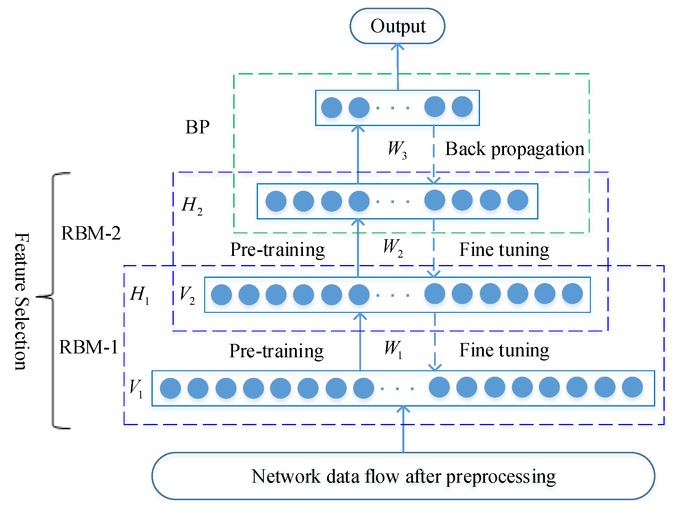
4.3. Training Classifier

The method for training classifier is a two-phase hybrid approach: unsupervised clustering and supervised learning. First, the unsupervised clustering algorithm MDPCA is utilized to divide the original training dataset into K subsets D C 1 ,   D C 2 , , D C K . Next, the DBNs initialize the network parameters through the unsupervised pre-training of BernoulliRBM, and then use the back-propagation algorithm to fine tune the network connection weights. We use the K subsets D C 1 ,   D C 2 , , D C K from the training dataset to train the K sub-DBN classifiers. Each subset D C i ( where i = 1 , 2 , , K ) is assigned to train the corresponding D B N i ( where i = 1 , 2 , , K ) . These DBNs are different from each other because they have been trained on different subsets. Each DBN has one input layer, three hidden layers, and one output layer. Three hidden layers automatically learn features from each training subset. The network structures of each DBN in the NSL-KDD and UNSW-NB15 datasets are 122-40-20-10-5 and 196-80-40-20-10, respectively.

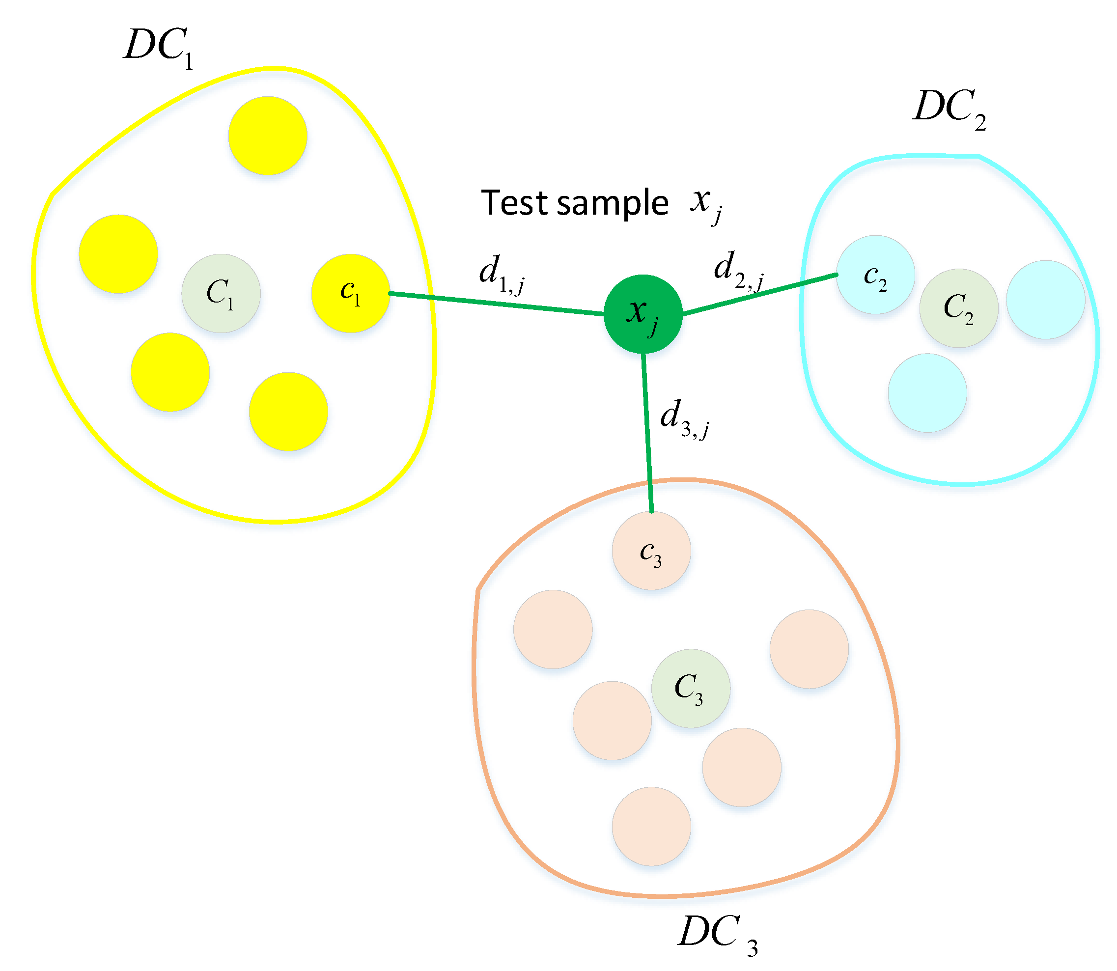
4.4. Attack Recognition

After completing the above steps, we obtain clusters of training datasets, which are divided into K disjoint subsets D C 1 ,   D C 2 , , D C K . These clusters are used to calculate the fuzzy membership matrix U = μ i , j , i = 1 , 2 , , K ; j = 1 , 2 , , N of the test samples associated with each cluster. For each test sample x j , we use the nearest neighbor sample c i of the ith cluster to calculate the fuzzy membership degree μ i , j according to Equation (14). Once these sub-DBNs classifiers have been trained on their training subsets, the test data are applied to each trained classifier D B N i ( w h e r e i = 1 , 2 , , K ) to detect and identify normal and intrusion network traffic. The predicted values of each sub- D B N i classifier are aggregated according to the fuzzy membership degree μ i , j . The output of test sample x j in each sub- D B N i classifier is defined as D B N i ( x j ) . The fuzzy aggregate output of each test sample x j can be computed as follows:
O u t = i = 1 K μ i , j · D B N i ( x j ) ,
where K is the number of clusters and represents the number of sub-DBNs classifiers.
The predictions of these sub-DBNs classifiers are aggregated into the final output of the intrusion detection system and used to detect attack categories. The proposed hybrid approach for intrusion detection is detailed in Algorithm 3.
Algorithm 3 MDPCA-DBN (Modified Density Peak Clustering Algorithm and Deep Belief Networks)
Input: Dataset S, cluster number K, Gaussian kernel parameter σ .
Output: the final classification results.
 1: Data collection: a training dataset and a testing dataset.
 2: Data preprocessing: feature mapping and data normalization.
 3: According to Algorithm 1, MDPCA is used to divide the original training dataset into K subsets
   D C 1 , D C 2 , , D C K .
 4: According to Algorithm 2, each training subset D C i is used to train the corresponding classifier
   D B N i .
 5: Caculate the fuzzy membership matrix U of test samples according to Equation (14).
 6: Test sample x j is tested on each trained D B N i classifier. The predictions of these D B N i classifiers
  are fuzzy aggregated according to Equation (28), and the final classification results are output.
 7: return the final classification results.

5. Experimental Results and Analysis

Experiments were carried out to evaluate the performance of the proposed model. We used three different datasets from the NSL-KDD and UNSW-NB15 datasets. We compared the results of the proposed model with other well-known detection methods. The proposed system was implemented in the Tensorflow environment on a ThinkStation with 64 GB RAM, Intel E5-2620 CPU and 64-bit Windows 10 operating system.

5.1. Performance Evaluation

To evaluate the performance of the proposed intrusion detection model, we used several widely applied metrics: accuracy, detection rate (DR), precision, recall, false positive rate (FPR), and F1-score. These metrics can be calculated based on four basic metrics of the confusion matrix, as shown in Table 1: True Positive (TP), True Negative (TN), False Positive (FP), and False Negative (FN). TP and TN indicate that the attack and normal records are correctly classified, respectively; FP represents a normal record that is incorrectly predicted as an attack; and FN represents an attack record that is incorrectly classified as a normal record.
Accuracy is the proportion of all predictions that are correctly identified as “Attack record” and “Normal record”. Accuracy is the most intuitive performance measure of an intrusion detection system. It directly reflects the superiority of the system. Accuracy is defined as follows:
A c c u r a c y = T P + T N T P + T N + F P + F N .
The detection rate (DR) is the proportion of the actual attack records that are correctly classified. DR is an important value for measuring the performance of the intrusion detection system. DR is defined as follows:
D R = T P T P + F N .
Precision is the proportion of all predicted attack records that are actually attack records. Precision is defined as follows:
P r e c i s i o n = T P T P + F P .
Recall is a measure of coverage and can indicate the ratio of the actual attack records that are correctly identified. Recall is also considered as the detection rate. With a certain accuracy, the recall rate of the classifier is required to be as high as possible. The recall is defined as follows:
R e c a l l = T P T P + F N .
The false positive rate (FPR) generally indicates the probability that normal records are incorrectly predicted as attack records. The FPR affects the performance of the intrusion detection system. The FPR is defined as follows:
F P R = F P F P + T N .
The F1-score is the harmonic mean of precision and recall. In other words, it can be interpreted as a weighted average of the precision and recall. The F1-score takes false positives and false negatives into account. The F1-score is usually more useful than accuracy, especially if you have an imbalanced class distribution. The F1-score is defined as follows:
F 1 s c o r e = 2 ( P r e c i s i o n R e c a l l ) P r e c i s i o n + R e c a l l = 2 T P 2 T P + F P + F N .

5.2. Description of the Benchmark Datasets

Currently, only few public benchmarks in the intrusion detection domain can be utilized to evaluate the performance of the IDS, such as KDD Cup 99 [46,47], NSL-KDD [21,22], UNSW-NB15 [25,26,27], ADFA [48], Kyoto 2006+ [49], ISCXIDS2012 [50], and CICIDS2017 [51]. The KDD Cup 99 dataset is from UCI (University of California, Irvine) Machine Learning Repository and is an upgraded version of the DARPA98 dataset. The KDD Cup 99 dataset has a large size and includes a huge number of duplicate and redundant records. The huge duplicate records can cause the classifier to bias toward the frequently occurring records. The NSL-KDD dataset is a modified version of the KDD Cup 99 dataset and removes redundant, duplicate and irrelevant data records in the KDD Cup 99 dataset. UNSW-NB15 is a new dataset created by the Cyber Range Lab of the Australian Cyber Security Center (ACCS) in 2015 through the IXIA PerfectStorm tool to generate a hybrid of real modern normal activities and synthetic contemporary attacks. The UNSW-NB15 dataset is more in line with today’s complex network environments. The ADFA dataset covers Linux and Windows system logs and is designed for HIDS (Host-based Intrusion Detection System) evaluation. In addition, Kyoto 2006+, ISCXIDS2012 and CICIDS2017 datasets contain only two types of data records, normal and abnormal. Therefore, we selected the NSL-KDD and UNSW-NB15 datasets to evaluate the proposed method.

5.2.1. NSL-KDD Dataset

The NSL-KDD is the most widely used dataset for evaluating intrusion detection performance. The NSL-KDD is derived from the original KDD Cup 99 dataset presented by Tavallaee et al. [47]. The NSD-KDD dataset removes duplicate and redundant records in the KDD Cup 99 dataset and is more suitable for evaluating the performance of intrusion detection system. There are five classes in the NSL-KDD dataset: v Normal, Probe, Denial of Service (DoS), User to Root (U2R), and Remote to Local (R2L) (Table 2).
The NSL-KDD dataset is unbalanced, with fewer U2R and R2L records, but more Normal and DoS records. We used three datasets in the NSL-KDD dataset to evaluate intrusion detection performance: KDDTrain+_20Percent.txt (a 20% subset of the KDDTrain+.txt file), KDDTest+.txt (the full NSL-KDD test set), and KDDTest-21.txt (a subset of the KDDTest+.txt file which has removed records with difficulty level 21). In our experiments, KDDTrain+_20Percent is used as a training set, and KDDTest+ and KDDTest-21 are used as test sets. Table 3 shows the number of records for each category on the NSL-KDD dataset.

5.2.2. UNSW-NB15 Dataset

The UNSW-NB15 is a new dataset that reflects real modern normal activities and contains synthetic contemporary attack behaviors [26]. This dataset is completely different from NSL-KDD, which reflects a more modern and complex threat environment. The raw network packet of the UNSW-NB15 dataset was created by the Tcpdump tool, and then 49 features with the class label were generated by Argus, Bro-IDS tool and 12 algorithms [27]. The full dataset contains a total of 25,400,443 records. The partition of the dataset is configured as a training set and a test set, namely, UNSW_NB15_training-set.csv and UNSW_NB15_testing-set.csv, respectively. The number of features in the partitioned dataset [26] is different from the number of features in the full dataset [25]. The partitioned dataset has only 43 features with the class label, removing 6 features (i.e. “srcip”, “sport”, “dstip”, “dsport”, “Stime” and “Ltime”) from the full dataset. There are ten different class labels in the partitioned dataset, one normal and nine attacks, namely, Generic, Exploits, Fuzzers, DoS, Reconnaissance (Reconn), Analysis, Backdoor, Shellcode and Worms. We used a stratified sampling method to randomly select 20% of the records from the UNSW_NB15_training-set and UNSW_NB15_testing-set datasets as training and test datasets. The training dataset consists of 35,069 records, whereas the testing dataset contains 16466 records. Table 4 shows in detail the class distribution of the UNSW-NB15 subset.

5.3. Experimental Setup

In the proposed MDPCA-DBN model, the MDPCA divides the training dataset into several subsets according to the feature similarity. An unreasonable subset will seriously affect the detection performance of the proposed model. The number of clusters K determines the division of clustering subsets and directly affects the detection performance. If the value of K is too large, the integrity of the original dataset will be destroyed and the detection accuracy will decrease. The appropriate K can divide the original dataset into more reasonable subsets and, to a certain extent, break the imbalance of the training dataset, thus achieving higher detection accuracy. We calculated the decision graph and γ sorting graph of the MDPCA algorithm according to Equation (10), and determined the number of subsets according to the number of discrete points. Figure 5 and Figure 6 show the decision graph and γ sorting graph on the NSL-KDD and UNSW-NB15 datasets, respectively. Figure 5a and Figure 6a show the relationship between the local density ρ and distance δ of each training sample. Figure 5b and Figure 6b show the γ i = ρ i δ i graph sorted in descending order. Rodriguez et al. [24] pointed out that the clustering centers have a high local density ρ and maximum distance δ , that is, those with larger γ values are clustering centers. The descending order of γ values provides the number of clustering centers to be selected. The γ value of non-clustering centers is relatively smooth, while the γ value from the non-clustering center to the clustering center has a significant jump. As can be seen from Figure 5b, there are two discrete jump points (marked red and green), so the optimal number of clusters on the NSL-KDD dataset is 2, and the data points corresponding to the red and green points are clustering centers. In Figure 6b, there are two discrete jump points (marked red and green) with large spacing, so the optimal clustering number on the UNSW-NB15 dataset is 2, and the data points corresponding to the red and green points are clustering centers.
Based on the experiment, we used the network structure and parameters that achieved the highest detection accuracy. The optimal network structures of the proposed model on the NSL-KDD and UNSW-NB15 datasets are 122-40-20-10-5 and 196-80-40-20-10, respectively. The Gaussian kernel parameter σ projects the original dataset into high dimensional space so that the spatial distribution of the original dataset is changed. The Gaussian kernel parameter σ varies between 1 and 300. Through a grid search on the NSL-KDD and UNSW-NB15 datasets, we found that the best σ values were 250 and 50, respectively. The proposed model uses the ReLU6 [52] activation function, 1000 iterations, 0.01 learning rate and Adam learning algorithm. We experimented on both datasets with the optimal K and σ values to evaluate the intrusion detection performance of the proposed model. These results are shown in Table 5 and Table 6. Table 7, Table 8 and Table 9 show the confusion matrix of the MDPCA-DBN on the NSL-KDD and UNSW-NB15 data sets, respectively.
Based on the above research results, to demonstrate the superiority of the proposed model, six currently well-known intrusion detection models were established using the NSL-KDD and UNSW-NB15 datasets. The comparison results are shown in Table 10, Table 11 and Table 12. In addition, the performance of the proposed model was further compared with other state-of-the-art models. Table 13 depicts the comparison results based on NSL-KDD (KDDTest+), NSL-KDD (KDDTest-21), and UNSW-NB15 datasets.

5.4. Results and Discussion

The optimal K and σ values for each dataset are shown in Table 5 and Table 6. The optimal K value on the NSL-KDD (KDDTest+), NSL-KDD (KDDTest-21), and UNSW-NB15 datasets is 2. A value of 2 for K implies that MDPCA can divide the original data into normal and attack records. The training dataset is divided into two subsets, which reduces the imbalance of the training dataset and improves the detection accuracy of the intrusion detection system. MDPCA-DBN has the same training set on the NSL-KDD (KDDTest+) and NSL-KDD (KDDTest-21) datasets, but the detection accuracy of the latter is lower than that of the former. The main reason is that the latter’s test set does not include records with difficulty level of 21 out of 21, and the proportion of unknown attacks is increasing.
Table 7, Table 8 and Table 9 show the confusion matrix of MDPCA-DBN with the optimal K and σ values on the NSL-KDD and UNSW-NB15 datasets. As can be seen in Table 5, the detection rates of U2R and R2L are relatively low. The main reason may be that there are too few samples of U2R and R2L in the training dataset (11 and 209 samples, respectively), and almost half of the U2R and R2L attacks in the test dataset never appear in the training dataset, such as httptunnel, sqlattack, etc. From the results in Table 7 and Table 8 we can infer that the attack features of U2R and R2L are similar to those of Normal. For example, snmpgetattack and Normal records have almost the same features. As a result, the U2R and R2L attack records provide less information for the MDPCA-DBN classifier, and most U2R and R2L attack records are incorrectly marked as normal records. Table 6 shows that the detection rates of DOS, Analysis, Backdoor, and Worms attacks are very low. It can be inferred from the results in Table 9 that the features of these attacks are similar to those of Exploits attacks. As a result, DOS, Analysis, Backdoor, and Worms attacks are misclassified as Exploits attacks.

5.5. Comparative Study

We compared the results of the proposed model with some well-known classification methods such as K-Nearest Neighbor (KNN), Multinomial Naive Bayes (MultinomialNB), Random Forest (RF), Support Vector Machine (SVM), Artificial Neural Network (ANN), and Deep Belief Network (DBN). The proposed model is named MDPCA-DBN, which is used to distinguish it from other models. The optimal cluster number K and Gaussian kernel parameter σ were selected on the NSL-KDD and UNSW-NB15 datasets according to Table 5 and Table 6. We performed performance evaluation based on the five metrics introduced in Section 5.1. The results compared with six well-known classifiers are depicted in Table 10, Table 11 and Table 12.
As shown in Table 10, the proposed MDPCA-DBN has the best overall accuracy, recall, precision, F1-score and FPR on the NSL-KDD (KDDTest+) dataset. In addition, our proposed model also achieved the best detection rate in the Normal and U2R classes. ANN has a slightly better detection rate in the DoS class compared to MDPCA-DBN (2.42% more). Moreover, MultinomialNB has 8.67% and 4.97% higher detection rates in Probe and R2L classes than MDPCA-DBN, respectively, but MDPCA-DBN has the best overall detection rate. Table 11 shows that MDPCA-DBN achieved the best overall performance, except for RF (slightly more 1.44% on the overall FPR). In addition, the detection rate of RF in the Normal class is 1.44% higher than that of the MDPCA-DBN, and the detection rate of DBN in the DoS class is 2.97% higher than that of MDPCA-DBN, but they are poor in other performances. MDPCA-DBN has the best detection rates on classes U2R and R2L. Table 10 and Table 11 show that MultinomialNB achieved the highest detection rate on the Probe class, which implies that the Probe attacks conform to the multinomial distribution. As shown in Table 10 and Table 11, all classifiers have very low detection rates on both U2R and R2L classes. Unlike DoS and Probe attacks, U2R has very few records (with only 11 records) in the NSL-KDD training dataset, which results in the classifier not being adequately trained; however, some of the attacks included in R2L class, such as snmpgetattack and snmpguess, exhibit highly similar features to those of normal records, which can cause the classifier to misclassify them as normal records.
Table 12 shows that MDPCA-DBN achieved the best overall performance compared to the other six well-known models, except for the overall recall rate (ANN slightly higher, 2.9%). MDPCA-DBN reaches the highest detection rate on the Normal, Generic, Reconnaissance, and Worms classes, but the detection rates are slightly worse on other classes. MultinomialNB achieves a highest detection rate of 73.84% in the DoS class, which implies that the DoS attack features are suitable for the multinomial distribution. RF reaches the highest detection rates on the Analysis, Backdoor, and Shellcode classes, but it is worse than the MDPCA-DBN on the overall F1-Score. In addition, we can see that all classifiers have low detection rates on the Analysis, Backdoor, and Worms classes, mainly because many contemporary attacks in the UNSW-NB15 dataset have similar behaviors, such as attack features of Analysis, Backdoor and Worms similar to those of Exploits.

5.6. Additional Comparison

To better demonstrate the performance of our proposed MDPCA-DBN model, we compared its performance with eight state-of-the-art intrusion detection techniques, namely, a Hybrid Spectral Clustering and Deep Neural Network Ensemble Algorithm (SCDNN) [30], Self-taught Learning Technique (STL) [53], Deep Neural Network (DNN) [54], Gaussian–Bernoulli RBM [38], Recurrent Neural Networks (RNN-IDS) [55], a Multiclass Cascade of Artificial Neural Network (CASCADE-ANN) [56], EM Clustering [27] and Decision Tree (DT) [27]. Table 13 demonstrates the comparison results of the proposed model with other models in terms of accuracy, DR (detection rate) and FPR (false positive rate) on the NSL-KDD (KDDTest+), NSL-KDD (KDDTest-21), and UNSW-NB15 datasets. As shown in Table 13, the proposed method achieved the best performance in terms of accuracy, detection rate and false positive rate on the NSL-KDD (KDDTest +) and NSL-KDD (KDDTest-21) datasets. It can be seen from the results that the proposed method achieved the highest accuracy of 90.21% and the highest detection rate of 96.22% on the UNSW-NB15 dataset, but the FPR is slightly worse. The CASCADE-ANN method proposed by Baig et al. [56] achieved a better false positive rate (with 4.05% more), but its accuracy and DR are worse than the proposed method.
Simulation results show that the proposed method outperformed on the NSL-KDD (KDDTest+), NSL-KDD (KDDTest-21), and UNSW-NB15 datasets in terms of Accuracy, DR and FPR except for CASCADE-ANN (FPR on UNSW-NB15 dataset). The results clearly demonstrate that the detection performances of the proposed model are more effective. However, because deep learning requires two stages of pre-training and fine-tuning, the proposed method requires more computation time than other shallow classification methods.

6. Conclusions and Future Work

In this paper, we propose a hybrid intrusion detection approach combining modified density peak clustering algorithm (MDPCA) and deep belief networks (DBNs). MDPCA is used to find similar features of complex and large-scale network data. According to the similarity of traffic features, large-scale network data are divided into several training subsets of different clustering centers. To a certain extent, MDPCA breaks the imbalance of multiclass records, reduces the complexity of training subsets, and makes the model achieve the best detection performance. DBN can automatically extract high-level abstract features from each training subset without a lot of heuristic rules and manual experience, and reduce data dimensions to avoid the curse of dimensions. As a deep learning approach, DBNs integrate feature extraction and classification modules into a system that can automatically extract features and classify them. This is an effective way to improve the detection performance. The classification performance of MDPCA-DBN was evaluated on the NSL-KDD (KDDTest+), NSL-KDD (KDDTest-21), and UNSW-NB15 datasets and compared with six well-known classifiers. In addition, the classification performance of MDPCA-DBN was also compared with other state-of-the-art classifiers on theNSL-KDD (KDDTest+), NSL-KDD (KDDTest-21), and UNSW-NB15 datasets. The experimental results show that the classification accuracy, detection rate and false positive rate of MDPCA-DBN are better than those of traditional methods.
Since fewer U2R and R2L attacks in the NSL-KDD dataset are recorded, and nearly half of the unknown attacks on the testing dataset never appear in the training dataset, it is difficult for all classifiers to detect U2R and R2L attacks. For future work, we plan to use the adversarial learning method to synthesize U2R and R2L attacks, thereby increasing training samples for U2R and R2L attacks. Through the adversarial learning method, similar unknown U2R and R2L attack records can be synthesized. As a result, the imbalance of five types of attack records is reduced and the detection accuracy of U2R and R2L attacks is improved. This can further improve the detection performance of the proposed model.

Author Contributions

Conceptualization, Y.Y. (Yanqing Yang), K.Z. and C.W.; Methodology, Y.Y. (Yanqing Yang), K.Z., C.W., X.N. and Y.Y. (Yixian Yang); Software, Y.Y. (Yanqing Yang); Validation, Y.Y. (Yanqing Yang), K.Z. and C.W.; Formal Analysis, X.N. and Y.Y. (Yixian Yang); Investigation, Y.Y. (Yanqing Yang) and K.Z.; Writing—Original Draft Preparation, Y.Y. (Yanqing Yang); Writing—Review and Editing, Y.Y. (Yanqing Yang), K.Z. and X.N.; Visualization, X.N.; Supervision, K.Z. and C.W.; and Project Administration, C.W.

Funding

This research was supported by the National Key R&D Program of China (2017YFB0802703) and National Natural Science Foundation of China (61602052).

Acknowledgments

The authors would like to thank the anonymous reviewers for their contribution to this paper.

Conflicts of Interest

The authors declare no conflict of interest.

References

  1. Hajisalem, V.; Babaie, S. A hybrid intrusion detection system based on ABC-AFS algorithm for misuse and anomaly detection. Comput. Netw. 2018, 136, 37–50. [Google Scholar] [CrossRef]
  2. Al-Yaseen, W.L.; Othman, Z.A.; Nazri, M.Z.A. Multi-level hybrid support vector machine and extreme learning machine based on modified K-means for intrusion detection system. Expert Syst. Appl. 2017, 67, 296–303. [Google Scholar] [CrossRef]
  3. Aljawarneh, S.; Aldwairi, M.; Yassein, M.B. Anomaly-based intrusion detection system through feature selection analysis and building hybrid efficient model. J. Comput. Sci. 2018, 25, 152–160. [Google Scholar] [CrossRef]
  4. Karami, A. An anomaly-based intrusion detection system in presence of benign outliers with visualization capabilities. Expert Syst. Appl. 2018, 108, 36–60. [Google Scholar] [CrossRef]
  5. Moustafa, N.; Creech, G.; Slay, J. Anomaly Detection System Using Beta Mixture Models and Outlier Detection. In Progress in Computing, Analytics and Networking; Springer: Berlin, Germany, 2018; pp. 125–135. [Google Scholar]
  6. Syarif, A.R.; Gata, W. Intrusion detection system using hybrid binary PSO and K-nearest neighborhood algorithm. In Proceedings of the 2017 11th International Conference on Information & Communication Technology and System (ICTS), Surabaya, Indonesia, 31 October 2017; pp. 181–186. [Google Scholar]
  7. Kuttranont, P.; Boonprakob, K.; Phaudphut, C.; Permpol, S.; Aimtongkhamand, P.; KoKaew, U.; Waikham, B.; So-In, C. Parallel KNN and Neighborhood Classification Implementations on GPU for Network Intrusion Detection. J. Telecommun. Electron. Comput. Eng. (JTEC) 2017, 9, 29–33. [Google Scholar]
  8. Kabir, E.; Hu, J.; Wang, H.; Zhuo, G. A novel statistical technique for intrusion detection systems. Future Gener. Comput. Syst. 2018, 79, 303–318. [Google Scholar] [CrossRef] [Green Version]
  9. Manzoor, I.; Kumar, N.; Akashdeep. A feature reduced intrusion detection system using ANN classifier. Expert Syst. Appl. 2017, 88, 249–257. [Google Scholar]
  10. Moon, D.; Im, H.; Kim, I.; Park, J.H. DTB-IDS: An intrusion detection system based on decision tree using behavior analysis for preventing APT attacks. J. Supercomput. 2017, 73, 2881–2895. [Google Scholar] [CrossRef]
  11. Aburomman, A.A.; Reaz, M.B.I. A survey of intrusion detection systems based on ensemble and hybrid classifiers. Comput. Secur. 2017, 65, 135–152. [Google Scholar] [CrossRef]
  12. Resende, P.A.A.; Drummond, A.C. A Survey of Random Forest Based Methods for Intrusion Detection Systems. ACM Comput. Surv. (CSUR) 2018, 51, 48. [Google Scholar] [CrossRef]
  13. Yadahalli, S.; Nighot, M.K. Adaboost based parameterized methods for wireless sensor networks. In Proceedings of the 2017 International Conference On Smart Technologies For Smart Nation (SmartTechCon), Karnataka, India, 17–19 August 2017; pp. 1370–1374. [Google Scholar]
  14. Roy, S.S.; Krishna, P.V.; Yenduri, S. Analyzing Intrusion Detection System: An ensemble based stacking approach. In Proceedings of the 2014 IEEE International Symposium on Signal Processing and Information Technology (ISSPIT), Noida, India, 15–17 December 2014; pp. 000307–000309. [Google Scholar]
  15. Hinton, G.E. Deep belief networks. Scholarpedia 2009, 4, 5947. [Google Scholar] [CrossRef]
  16. Hinton, G.E.; Osindero, S.; Teh, Y.W. A fast learning algorithm for deep belief nets. Neural Comput. 2006, 18, 1527–1554. [Google Scholar] [CrossRef] [PubMed]
  17. Wang, Z. Deep Learning-Based Intrusion Detection With Adversaries. IEEE Access 2018, 6, 38367–38384. [Google Scholar] [CrossRef]
  18. Xin, Y.; Kong, L.; Liu, Z.; Chen, Y.; Li, Y.; Zhu, H.; Gao, M.; Hou, H.; Wang, C. Machine Learning and Deep Learning Methods for Cybersecurity. IEEE Access 2018, 6, 35365–35381. [Google Scholar] [CrossRef]
  19. Huda, S.; Miah, S.; Yearwood, J.; Alyahya, S.; Al-Dossari, H.; Doss, R. A malicious threat detection model for cloud assisted internet of things (CoT) based industrial control system (ICS) networks using deep belief network. J. Parallel Distrib. Comput. 2018, 120, 23–31. [Google Scholar] [CrossRef]
  20. Ambusaidi, M.A.; He, X.; Nanda, P.; Tan, Z. Building an intrusion detection system using a filter-based feature selection algorithm. IEEE Trans. Comput. 2016, 65, 2986–2998. [Google Scholar] [CrossRef]
  21. UNB. NSL-KDD Dataset. Available online: https://www.unb.ca/cic/datasets/nsl.html (accessed on 10 December 2018).
  22. Dhanabal, L.; Shantharajah, S. A study on NSL-KDD dataset for intrusion detection system based on classification algorithms. Int. J. Adv. Res. Comput. Commun. Eng. 2015, 4, 446–452. [Google Scholar]
  23. Lopez-Martin, M.; Carro, B.; Sanchez-Esguevillas, A.; Lloret, J. Conditional variational autoencoder for prediction and feature recovery applied to intrusion detection in iot. Sensors 2017, 17, 1967. [Google Scholar] [CrossRef]
  24. Rodriguez, A.; Laio, A. Clustering by fast search and find of density peaks. Science 2014, 344, 1492–1496. [Google Scholar] [CrossRef] [Green Version]
  25. ACCS. UNSW-NB15 Dataset. Available online: https://www.unsw.adfa.edu.au/unsw-canberra-cyber/cybersecurity/ADFA-NB15-Datasets/ (accessed on 10 December 2018).
  26. Moustafa, N.; Slay, J. UNSW-NB15: A comprehensive data set for network intrusion detection systems (UNSW-NB15 network data set). In Proceedings of the 2015 IEEE Military Communications and Information Systems Conference (MilCIS), Canberra, Australia, 10–12 November 2015; pp. 1–6. [Google Scholar]
  27. Moustafa, N.; Slay, J. The evaluation of Network Anomaly Detection Systems: Statistical analysis of the UNSW-NB15 data set and the comparison with the KDD99 data set. Inf. Secur. J. Glob. Perspect. 2016, 25, 18–31. [Google Scholar] [CrossRef]
  28. Cha, Y.J.; Wang, Z. Unsupervised novelty detection–based structural damage localization using a density peaks-based fast clustering algorithm. Struct. Health Monit. 2018, 17, 313–324. [Google Scholar] [CrossRef]
  29. Li, L.; Zhang, H.; Peng, H.; Yang, Y. Nearest neighbors based density peaks approach to intrusion detection. Chaos Solitons Fractals 2018, 110, 33–40. [Google Scholar] [CrossRef]
  30. Ma, T.; Wang, F.; Cheng, J.; Yu, Y.; Chen, X. A Hybrid Spectral Clustering and Deep Neural Network Ensemble Algorithm for Intrusion Detection in Sensor Networks. Sensors 2016, 16, 1701. [Google Scholar] [CrossRef] [PubMed]
  31. Thing, V.L. IEEE 802.11 network anomaly detection and attack classification: A deep learning approach. In Proceedings of the 2017 IEEE Wireless Communications and Networking Conference (WCNC), San Francisco, CA, USA, 19–22 March 2017; pp. 1–6. [Google Scholar]
  32. Naseer, S.; Saleem, Y. Enhanced Network Intrusion Detection using Deep Convolutional Neural Networks. KSII Trans. Internet Inf. Syst. 2018, 12. [Google Scholar] [CrossRef]
  33. Tang, T.; Zaidi, S.A.R.; McLernon, D.; Mhamdi, L.; Ghogho, M. Deep Recurrent Neural Network for Intrusion Detection in SDN-based Networks. In Proceedings of the 2018 IEEE International Conference on Network Softwarization (NetSoft 2018), Montreal, ON, Canada, 25–29 June 2018. [Google Scholar]
  34. Shone, N.; Ngoc, T.N.; Phai, V.D.; Shi, Q. A deep learning approach to network intrusion detection. IEEE Trans. Emerg. Top. Comput. Intell. 2018, 2, 41–50. [Google Scholar] [CrossRef]
  35. Muna, A.H.; Moustafa, N.; Sitnikova, E. Identification of malicious activities in industrial internet of things based on deep learning models. J. Inf. Secur. Appl. 2018, 41, 1–11. [Google Scholar]
  36. Tamer Aldwairi, D.P.; Novotny, M.A. An evaluation of the performance of Restricted Boltzmann Machines as a model for anomaly network intrusion detection. Comput. Netw. 2018, 144, 111–119. [Google Scholar] [CrossRef]
  37. Li, C.; Wang, J.; Ye, X. Using a Recurrent Neural Network and Restricted Boltzmann Machines for Malicious Traffic Detection. NeuroQuantology 2018, 16. [Google Scholar] [CrossRef]
  38. Imamverdiyev, Y.; Abdullayeva, F. Deep Learning Method for Denial of Service Attack Detection Based on Restricted Boltzmann Machine. Big Data 2018, 6, 159–169. [Google Scholar] [CrossRef]
  39. Nguyen, B.; Morell, C.; De Baets, B. Supervised distance metric learning through maximization of the Jeffrey divergence. Pattern Recognit. 2017, 64, 215–225. [Google Scholar] [CrossRef]
  40. Hinton, G.E.; Salakhutdinov, R.R. Reducing the dimensionality of data with neural networks. Science 2006, 313, 504–507. [Google Scholar] [CrossRef] [PubMed]
  41. Hinton, G. A practical guide to training restricted Boltzmann machines. Momentum 2010, 9, 926. [Google Scholar]
  42. Fischer, A.; Igel, C. Training restricted Boltzmann machines: An introduction. Pattern Recognit. 2014, 47, 25–39. [Google Scholar] [CrossRef] [Green Version]
  43. Swersky, K.; Chen, B.; Marlin, B.; De Freitas, N. A tutorial on stochastic approximation algorithms for training restricted Boltzmann machines and deep belief nets. In Proceedings of the 2010 Information Theory and Applications Workshop (ITA), San Diego, CA, USA, 31 January–5 February 2010; pp. 1–10. [Google Scholar]
  44. Hinton, G.E. Training products of experts by minimizing contrastive divergence. Neural Comput. 2002, 14, 1771–1800. [Google Scholar] [CrossRef] [PubMed]
  45. Tieleman, T. Training restricted Boltzmann machines using approximations to the likelihood gradient. In Proceedings of the 25th international conference on Machine Learning, Helsinki, Finland, 5–9 July 2018; ACM: New York, NY, USA, 2008; pp. 1064–1071. [Google Scholar] [Green Version]
  46. KDDCup. KDD Cup Dataset. Available online: http://archive.ics.uci.edu/ml/datasets/kdd+cup+1999+data (accessed on 10 December 2018).
  47. Tavallaee, M.; Bagheri, E.; Lu, W.; Ghorbani, A.A. A detailed analysis of the KDD CUP 99 data set. In Proceedings of the 2009 IEEE Symposium on Computational Intelligence for Security and Defense Applications, Ottawa, ON, Canada, 8–10 July 2009; pp. 1–6. [Google Scholar]
  48. Creech, G. Developing a High-Accuracy Cross Platform Host-Based Intrusion Detection System Capable of Reliably Detecting Zero-Day Attacks. Ph.D. Thesis, University of New South Wales, Canberra, Australia, 2014. [Google Scholar]
  49. Song, J.; Takakura, H.; Okabe, Y.; Eto, M.; Inoue, D.; Nakao, K. Statistical analysis of honeypot data and building of Kyoto 2006+ dataset for NIDS evaluation. In Proceedings of the First Workshop on Building Analysis Datasets and Gathering Experience Returns for Security, Salzburg, Austria, 10–13 April 2011; pp. 29–36. [Google Scholar]
  50. Shiravi, A.; Shiravi, H.; Tavallaee, M.; Ghorbani, A.A. Toward developing a systematic approach to generate benchmark datasets for intrusion detection. Comput. Secur. 2012, 31, 357–374. [Google Scholar] [CrossRef]
  51. Sharafaldin, I.; Lashkari, A.H.; Ghorbani, A.A. Toward Generating a New Intrusion Detection Dataset and Intrusion Traffic Characterization. In Proceedings of the ICISSP 2018: 4th International Conference on Information Systems Security and Privacy, Funchal, Portugal, 22–24 January 2018; pp. 108–116. [Google Scholar]
  52. Maas, A.L.; Hannun, A.Y.; Ng, A.Y. Rectifier nonlinearities improve neural network acoustic models. Proc. ICML 2013, 30, 3. [Google Scholar]
  53. Javaid, A.; Niyaz, Q.; Sun, W.; Alam, M. A deep learning approach for network intrusion detection system. In Proceedings of the 9th EAI International Conference on Bio-Inspired Information and Communications Technologies (formerly BIONETICS), New York, NY, USA, 2–5 December 2016; pp. 21–26. [Google Scholar]
  54. Tang, T.A.; Mhamdi, L.; McLernon, D.; Zaidi, S.A.R.; Ghogho, M. Deep learning approach for network intrusion detection in software defined networking. In Proceedings of the 2016 International Conference on Wireless Networks and Mobile Communications (WINCOM), Fez, Morocco, 26–29 October 2016; pp. 258–263. [Google Scholar]
  55. Yin, C.; Zhu, Y.; Fei, J.; He, X. A deep learning approach for intrusion detection using recurrent neural networks. IEEE Access 2017, 5, 21954–21961. [Google Scholar] [CrossRef]
  56. Baig, M.M.; Awais, M.M.; El-Alfy, E.S.M. A multiclass cascade of artificial neural network for network intrusion detection. J. Intell. Fuzzy Syst. 2017, 32, 2875–2883. [Google Scholar] [CrossRef]
Figure 1. The nearest neighbor distance of the test sample in each cluster.
Applsci 09 00238 g001
Figure 2. The graphical representation of an RBM with m visible nodes and n hidden nodes.
Applsci 09 00238 g002
Figure 3. DBNs structural model.
Applsci 09 00238 g003
Figure 4. The framework of the proposed hybrid model.
Applsci 09 00238 g004
Figure 5. Decision graph and γ sorting graph of MDPCA algorithm on the NSL-KDD dataset.
Applsci 09 00238 g005
Figure 6. Decision graph and γ sorting graph of MDPCA algorithm on the UNSW-NB15 dataset.
Applsci 09 00238 g006
Table 1. The four basic metrics of the confusion matrix.
Test Result Positive
(Predicted as an Attack)
Test Result Negative
(Predicted as a Normal Record)
Actual positive class (Attack record)True positive (TP)False negative (FN)
Actual negative class (Normal record)False positive (FP)True negative (TN)
Table 2. Categories of the NSL-KDD dataset records.
CategoriesDescriptionExamples
Normalinclude data with no attack.normal
Probeinclude attacks in which attackers try to scan the computer networks with the purpose of collecting information and finding out vulnerabilities.ipsweep, nmap, portsweep, satan, saint, mscan
DoSinclude attacks in which attackers try to prevent legitimate users of a service from using the serviceback, land, neptune, pod, smurf, teardrop, apache2, mailbomb, udpstorm, processtable
U2Rinclude attacks in which attackers have local access to the victim target machine and try to get super user privileges.perl, rootkit, loadmodule, buffer_overflow, httptunnel, ps, sqlattack, xterm
R2Linclude attacks in which attackers do not have a local account and try to gain access by sending packets to the target host over the internet.ftp_write, guess_passwd, multihop, phf, imap, spy, warezclient, warezmaster, named, xsnoop, xlock, sendmail, worm, snmpgetattack, snmpguess
Table 3. The class distribution of the NSL-KDD dataset.
CategoryTraining DatasetTesting Dataset
KDDTrain+_20PercentKDDTest+KDDTest-21
Normal13,44997112152
Probe228924212402
DoS923474584342
U2R11200200
R2L20927542754
Total25,19222,54411,850
Table 4. The class distribution of the UNSW-NB15 subset.
CategoryTraining DatasetTesting Dataset
UNSW_NB15_Training-Set 20%UNSW_NB15_Testing-Set 20%
Normal11,2007400
Generic80003774
Exploits66792226
Fuzzers36371212
DoS2453818
Reconnaissance2098699
Analysis400135
Backdoor349117
Shellcode22776
Worms269
Total35,06916,466
Table 5. Detection accuracy (%) with optimal parameters K and σ for NSL-KDD (KDDTest+) and NSL-KDD (KDDTest-21) datasets.
DatasetK σ NormalProbeDoSU2RR2LAccuracy
NSL-KDD (KDDTest+)225097.3873.9481.096.517.2582.08
NSL-KDD (KDDTest-21)225086.9463.268.756.34.9366.18
Table 6. Detection accuracy (%) with optimal parameters K and σ for UNSW-NB15 dataset.
K σ NormalGenericExploitsFuzzersDoSReconnaissance
25082.8596.9383.5144.3923.7276.68
AnalysisBackdoorShellcodeWormsAccuracy
0.000.8539.4711.1190.21
Table 7. Confusion matrix of NSL-KDD (KDDTest+) dataset with optimal parameters K and σ .
NormalProbeDoSU2RR2L
Normal94571865558
Probe4431790174131
DoS90696604869339
U2R18100136
R2L225513110475
Table 8. Confusion matrix of NSL-KDD (KDDTest-21) dataset with optimal parameters K and σ .
NormalProbeDoSU2RR2L
Normal18712176121
Probe7031518158122
DoS10765829850223
U2R17811128
R2L17701246962
Table 9. Confusion matrix of UNSW-NB15 dataset with optimal parameters K and σ .
NormalGenericExploitsFuzzersDoSReconnAnalysisBackdoorShellcodeWorms
Normal613121589061812848090
Generic13658976360030
Exploits37121859452302060143
Fuzzers2840205538798002240
DoS765891419440040
Reconn1001344145360010
Analysis008115210000
Backdoor106734310110
Shellcode31161021400300
Worms0071000001
Table 10. Comparison results for the NSL-KDD (KDDTest+) dataset (%).
ModelNormalProbeDoSU2RR2LAccuracyRecallPrecisionF1-ScoreFPR
KNN92.7859.482.253.53.5676.5164.1992.1675.687.22
MultinomialNB96.0382.6137.10.522.2278.7365.6495.6277.853.97
RF97.3758.5380.240.507.5576.4960.6996.8474.622.63
SVM92.8261.7174.850.000.0072.2856.7391.2669.977.18
ANN93.6858.6583.510.5013.2577.6165.4593.1976.896.32
DBN97.0469.8583.115.5012.5680.8268.5396.8480.262.96
MDPCA-DBN97.3873.9481.096.5017.2582.0870.5197.2781.752.62
Table 11. Comparison results for the NSL-KDD (KDDTest-21) dataset (%).
ModelNormalProbeDoSU2RR2LAccuracyRecallPrecisionF1-ScoreFPR
KNN68.4959.0869.813.503.5655.552.6288.2765.9331.51
MultinomialNB83.3282.8138.120.522.2260.0854.9393.6969.2516.68
RF88.3860.4566.080.5010.4256.8449.8495.0865.3911.62
SVM68.2661.4156.790.000.0047.3842.7485.8557.0731.74
ANN67.2456.4550.410.000.0045.040.0684.6454.3832.76
DBN71.7558.3371.720.5013.2557.4554.2889.6567.6228.25
MDPCA-DBN86.9463.2068.756.0034.9366.1861.5795.5174.8713.06
Table 12. Comparison results for the UNSW-NB15 dataset (%).
ClassKNNMultinomialNBRFSVMANNDBNMDPCA-DBN
Normal74.8162.076.8558.3663.8972.1282.85
Generic96.6396.2496.496.2195.5596.0896.93
Exploits74.4842.8177.6375.5287.7491.0283.51
Fuzzers42.3333.2551.3269.3168.9843.3244.39
DoS19.4473.8417.60.005.132.3223.72
Reconnaissance58.9436.3476.680.0063.3870.6776.68
Analysis1.480.03.70.000.000.000.00
Backdoor2.560.05.130.000.000.000.85
Shellcode14.470.051.320.000.000.0039.47
Worms11.110.011.110.000.000.0011.11
Accuracy85.3876.7587.5679.3683.2986.0290.21
Recall94.0188.7896.2996.4999.1297.3696.22
Precision82.0574.1183.673.9577.0881.0687.3
F1-score87.6380.7889.583.7386.7288.4691.54
FPR25.1938.023.1541.6436.1127.8817.15
Table 13. Comparison results based on NSL-KDD and UNSW-NB15 datasets (N/A means no available results, * Ranked first, ** Ranked second).
MethodDatasetAccuracy(%)DR(%)FPR(%)
SCDNN [30]NSL-KDD (KDDTest+)72.6457.48N/A
STL [53]NSL-KDD (KDDTest+)74.3862.99 **7.21 **
DNN [54]NSL-KDD (KDDTest+)75.75N/AN/A
Gaussian–Bernoulli RBM [38]NSL-KDD (KDDTest+)73.23N/AN/A
RNN-IDS [55]NSL-KDD (KDDTest+)81.29 **N/AN/A
MDPCA-DBNNSL-KDD (KDDTest+)82.08 *70.51 *2.62 *
SCDNN [30]NSL-KDD (KDDTest-21)44.5537.85N/A
STL [53]NSL-KDD (KDDTest-21)57.3452.73 **15.06 **
RNN-IDS [55]NSL-KDD (KDDTest+)64.67 **N/AN/A
MDPCA-DBNNSL-KDD (KDDTest-21)66.18 *61.57 *13.06 *
CASCADE-ANN [56]UNSW-NB1586.40 **86.74 **13.1 *
EM Clustering [27]UNSW-NB1578.47N/AN/A
DT [27]UNSW-NB1585.56N/AN/A
MDPCA-DBNUNSW-NB1590.21 *96.22 *17.15 **

