Prediction of Concrete Strength with P-, S-, R-Wave Velocities by Support Vector Machine (SVM) and Artificial Neural Network (ANN)


Abstract
1. Introduction
2. Ultrasonic Pulse Velocity Test
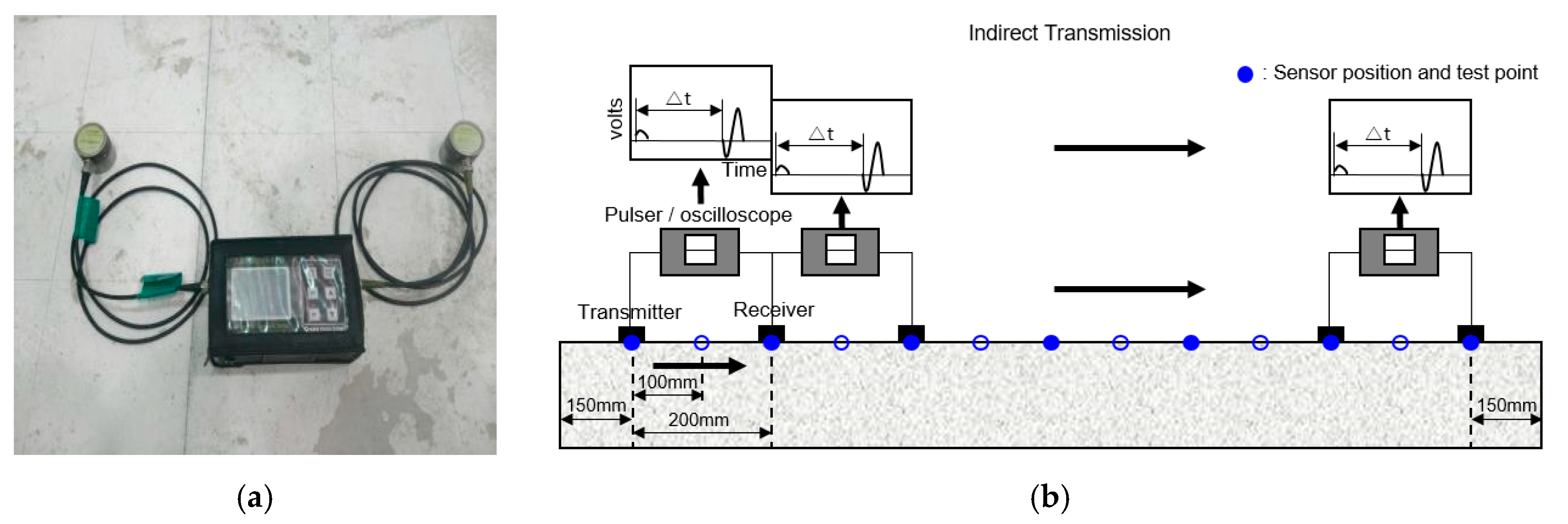
2.1. P-Wave Velocity (Vp) Measurement
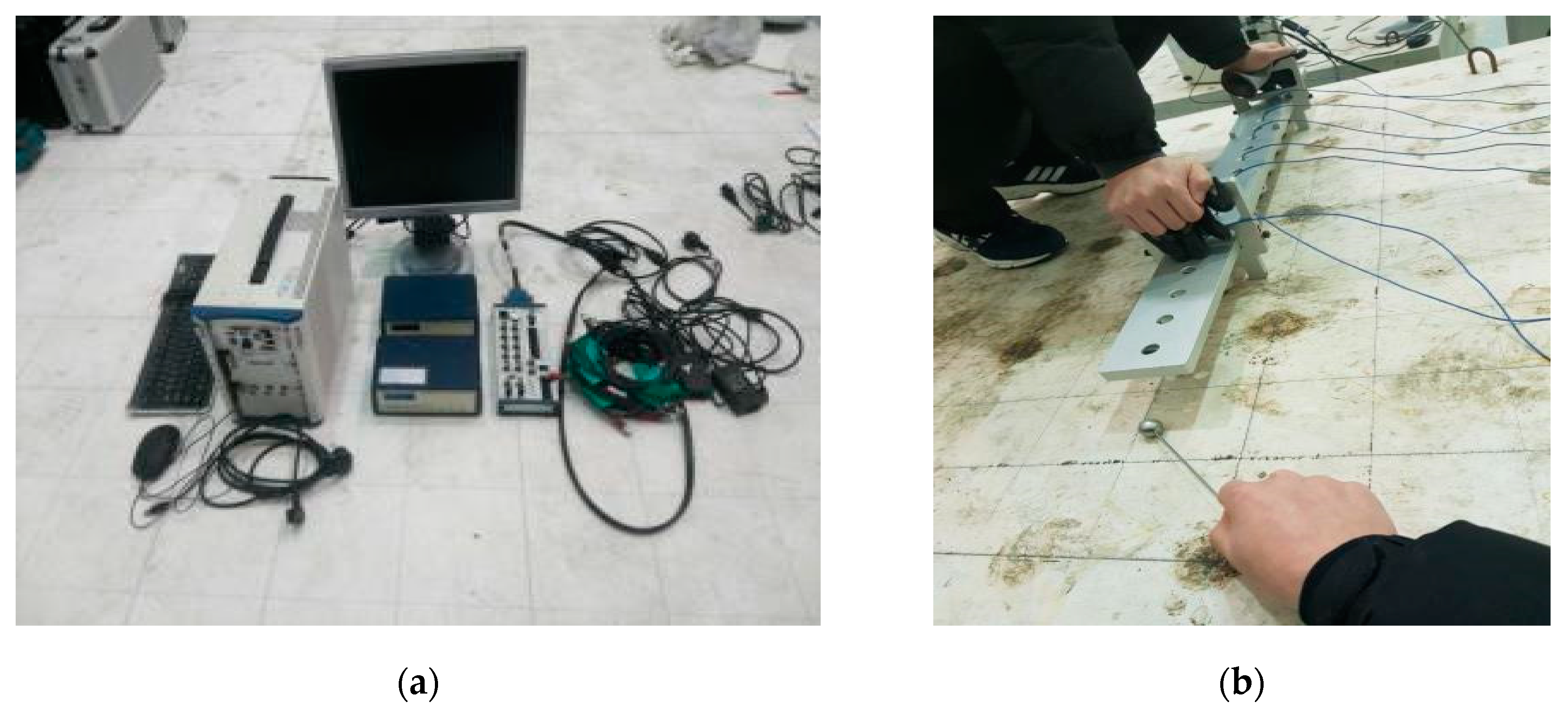
2.2. S-Wave Velocity (Vs) Measurement
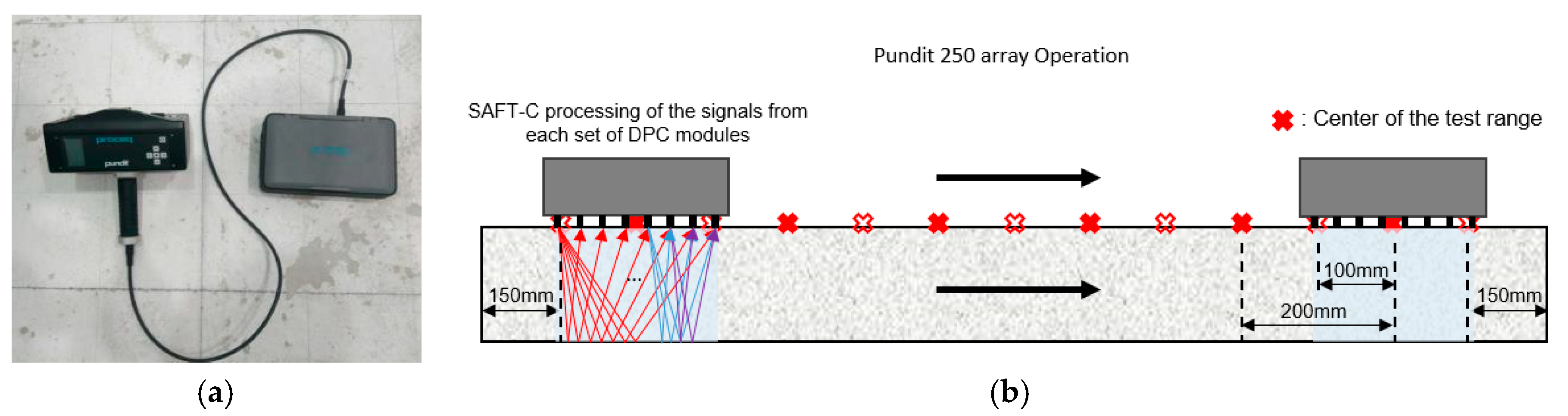
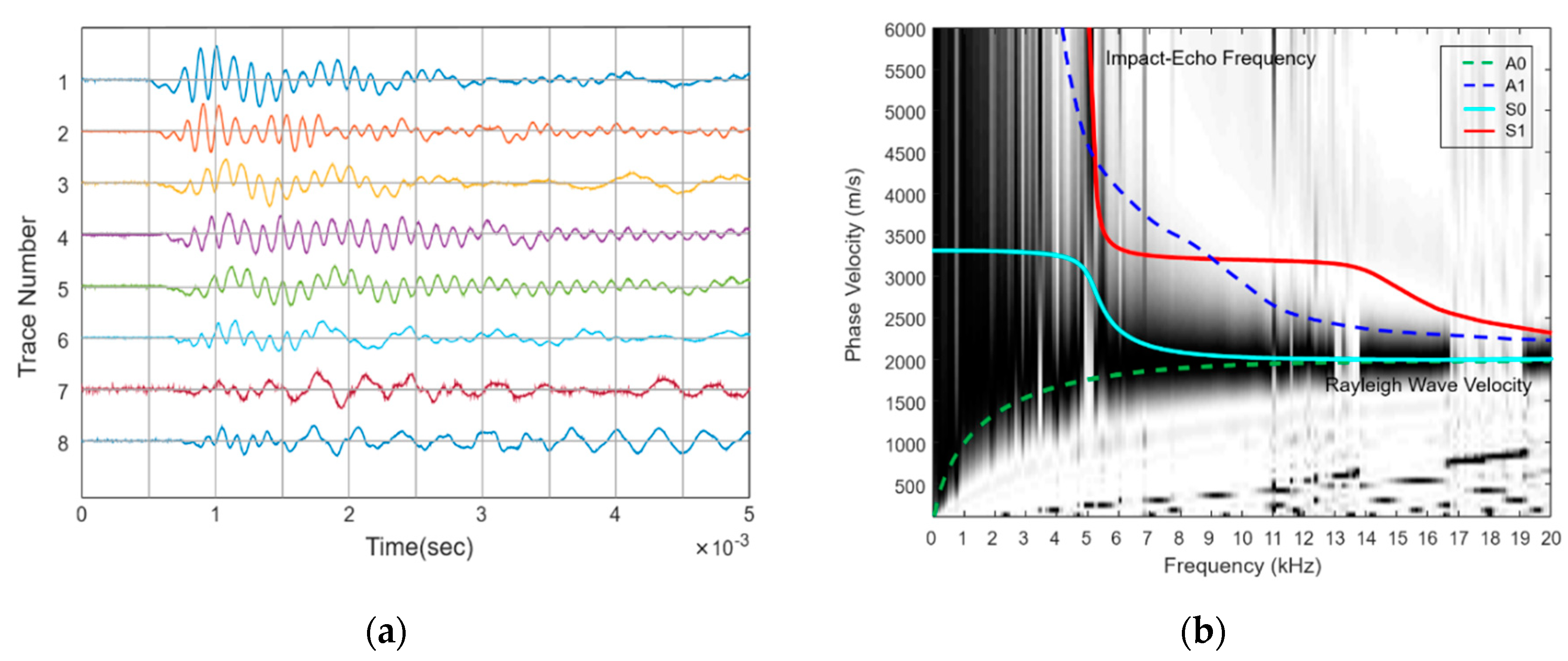
2.3. R-Wave Velocity (Vr) Measurement
3. Machine Learning Technique
3.1. Support Vector Machines and Model Development
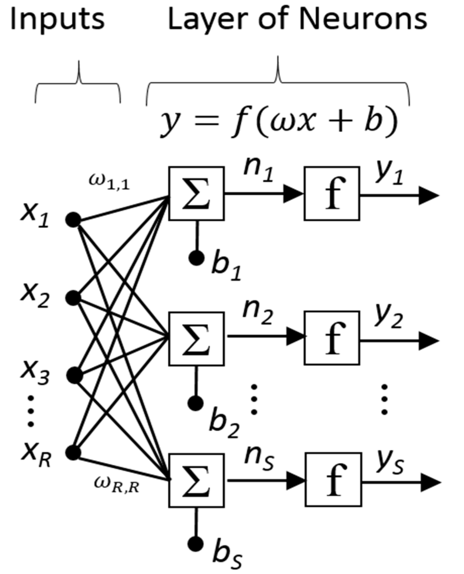
3.2. Artificial Neural Network (ANN) and Model Development
4. Experimental Method
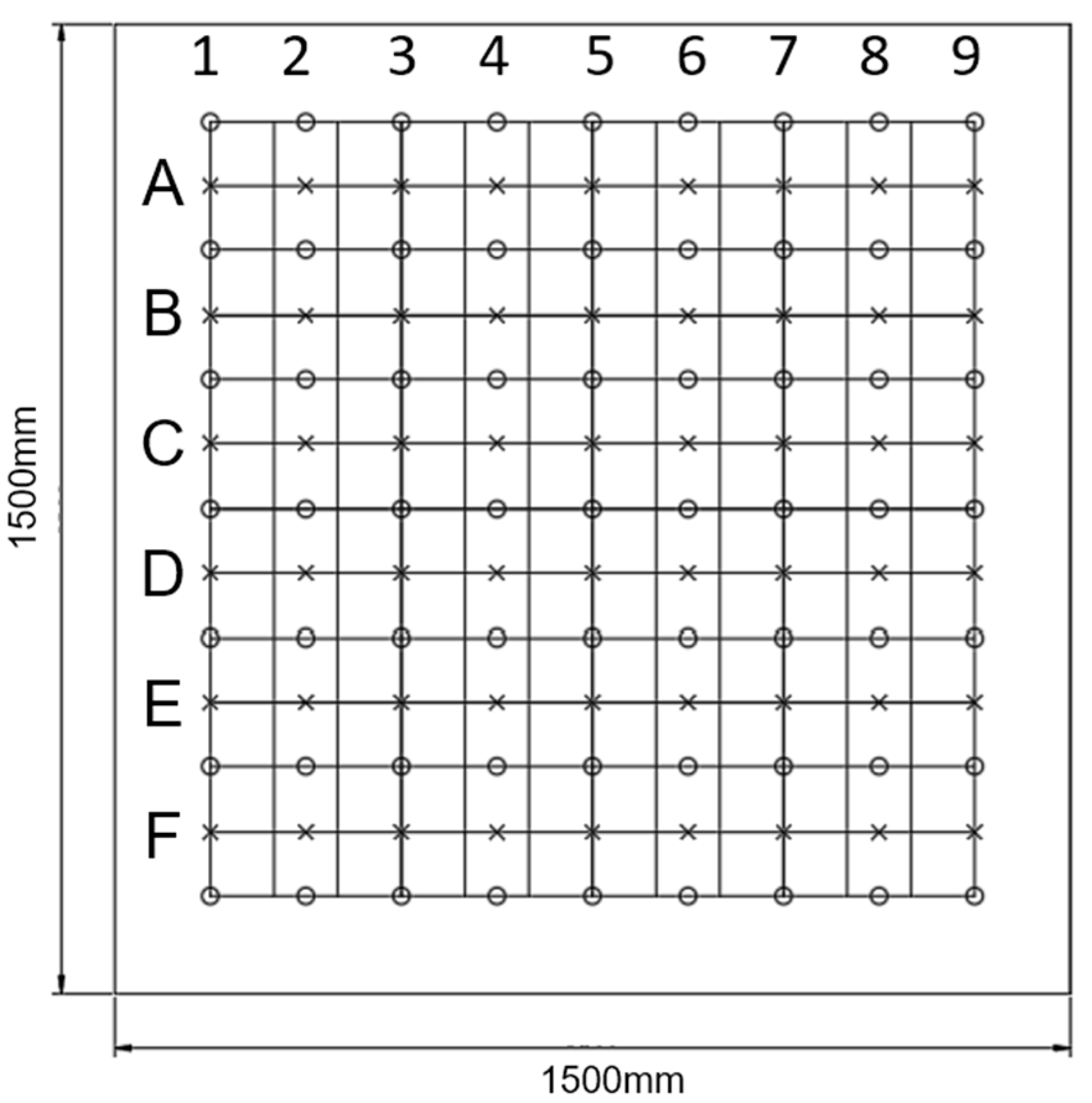
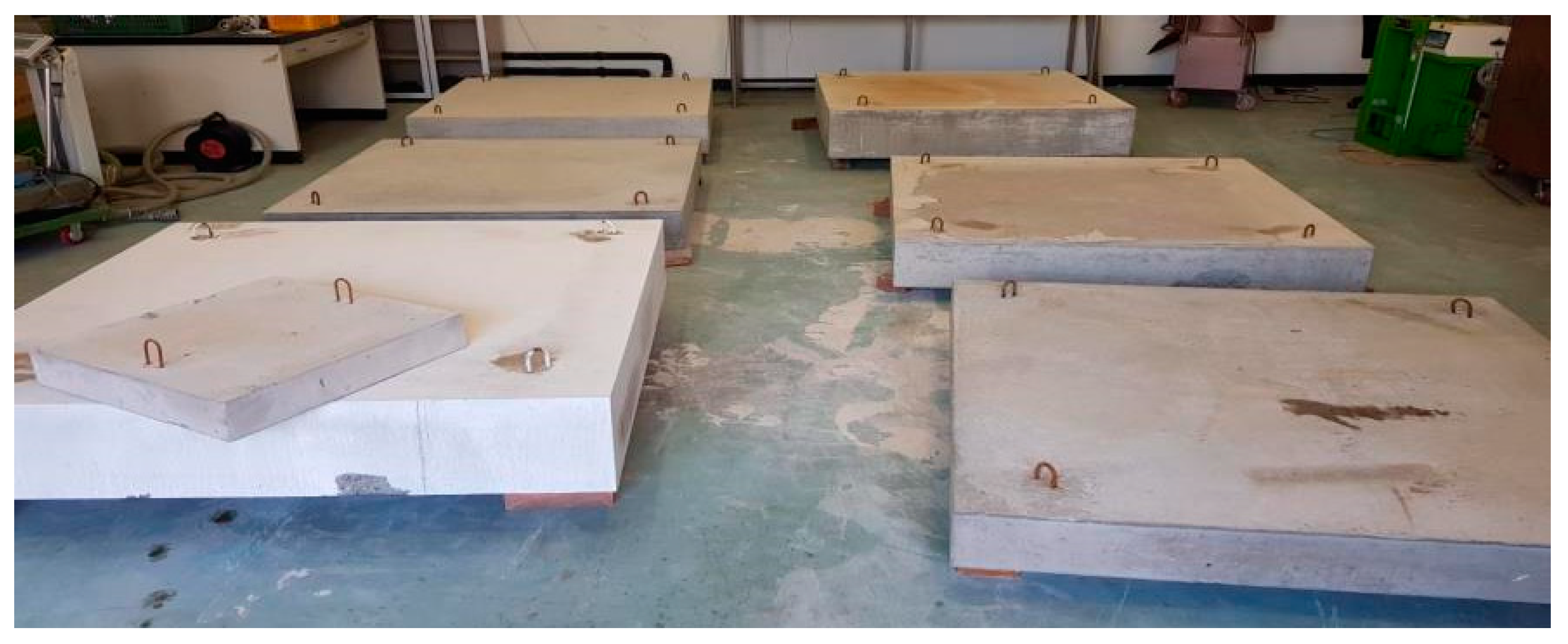
4.1. Test Specimen
4.2. Wave Velocity Measurements
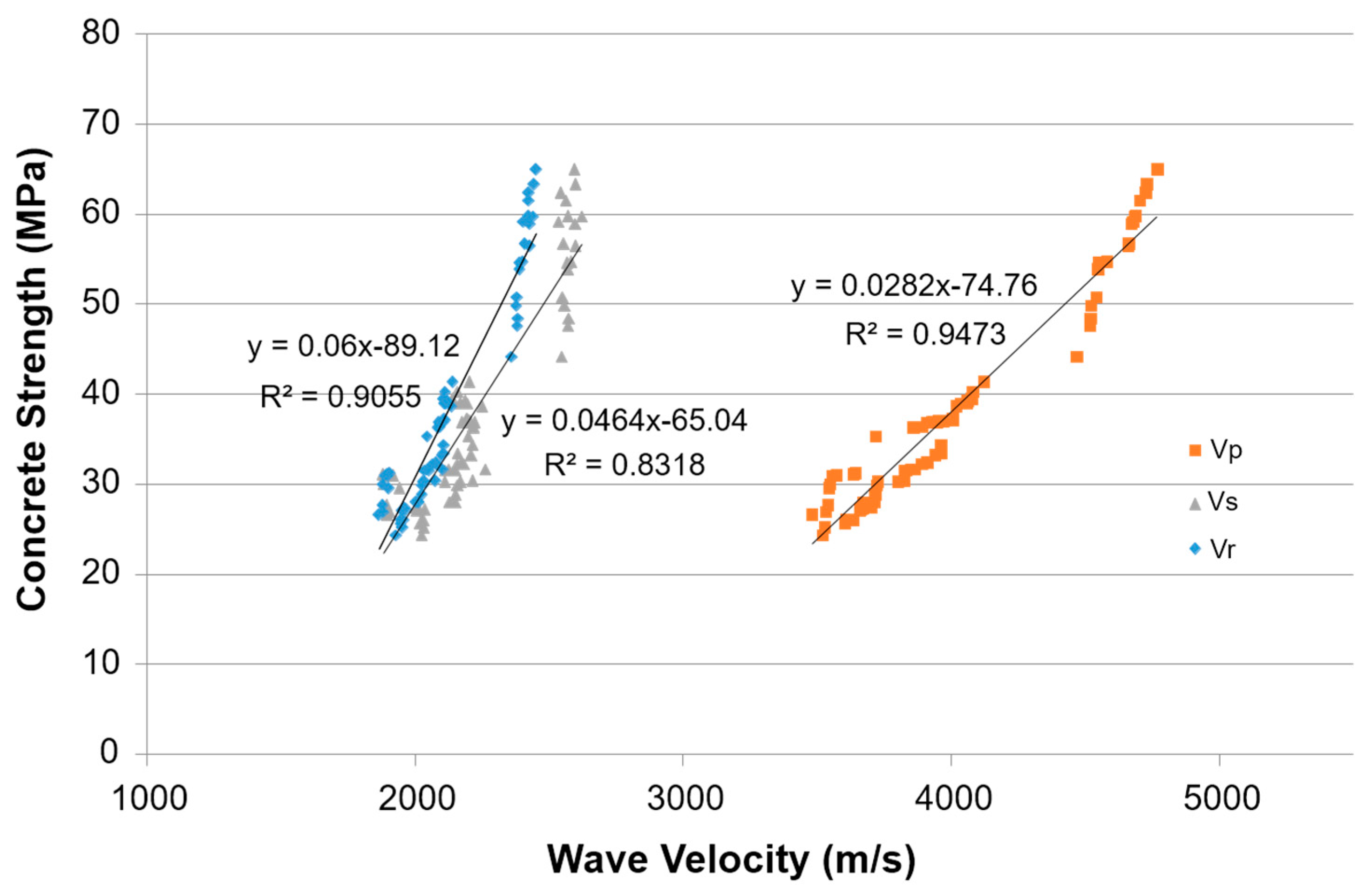
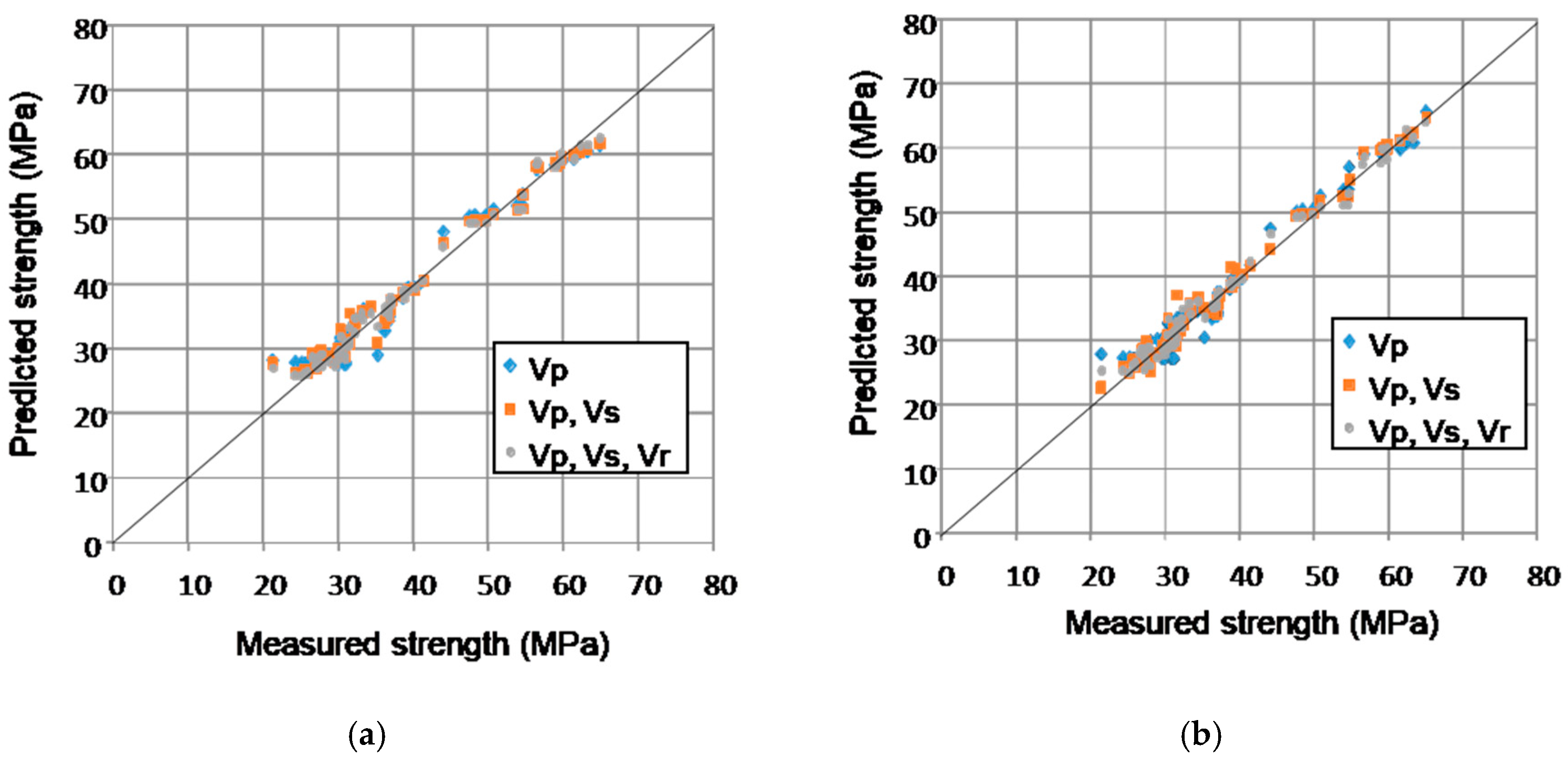
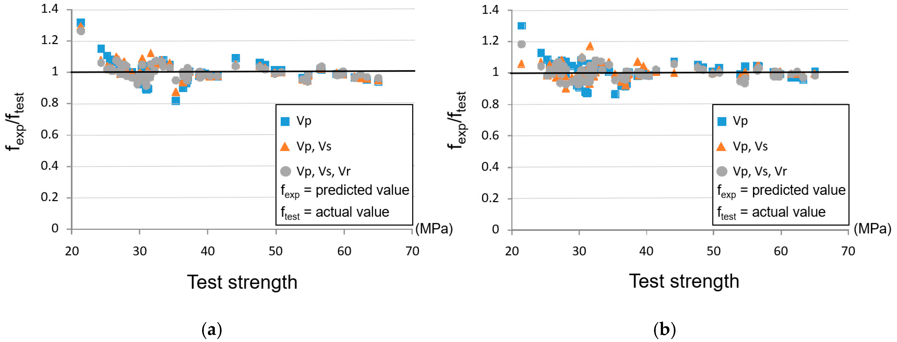
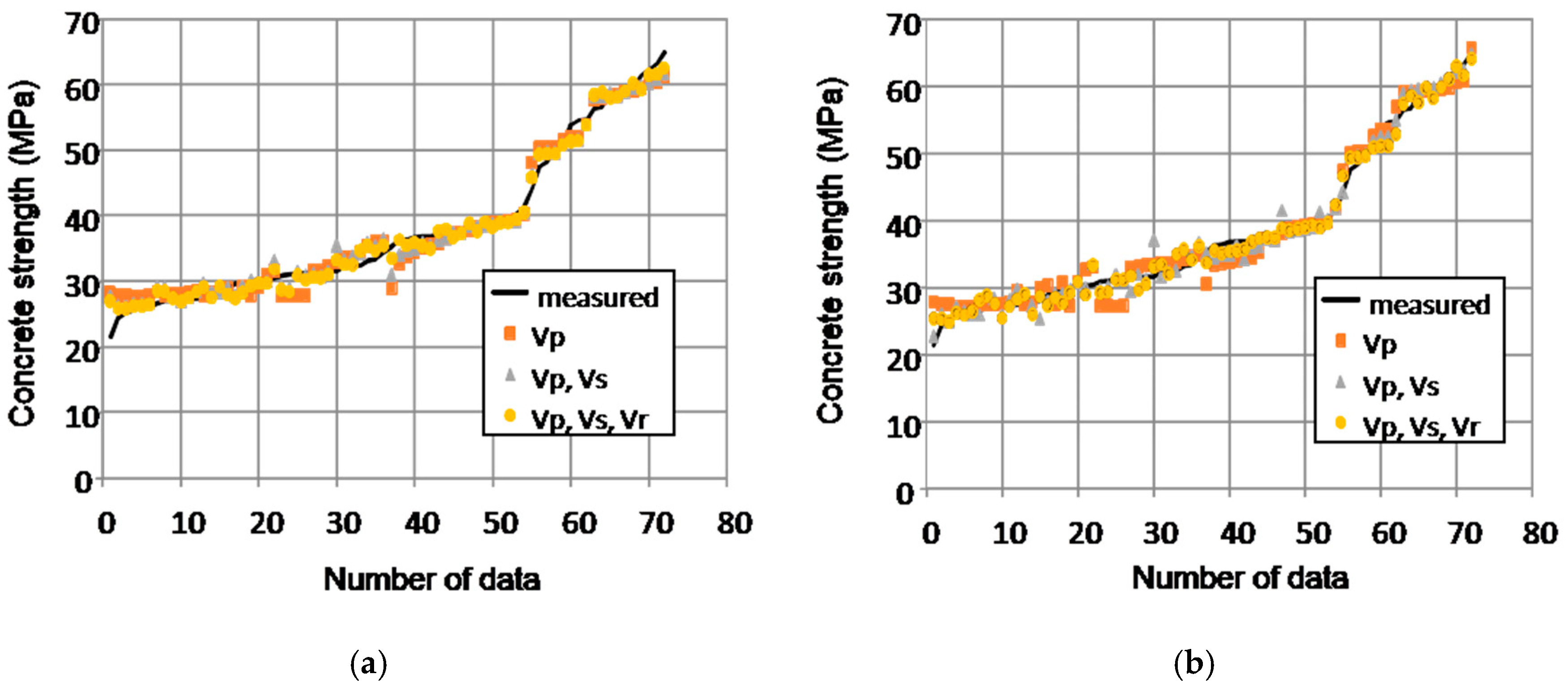
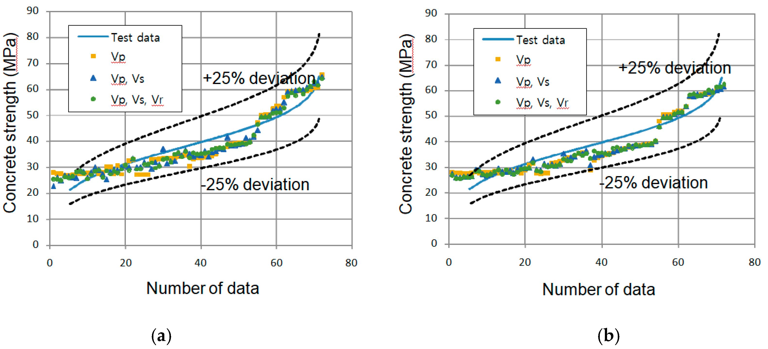
5. Analysis of Results
6. Conclusions
- In the prediction of concrete strength, the predictive models that used three types of ultrasonic velocities were more accurate than the models that used only one or two velocities, and they converged more quickly with smaller errors.
- The SVM model was able to obtain more accurate predictions than the ANN because of the less generalizable performances and over-fitting issues of ANNs.
- A slight change in the ultrasonic velocity was observed at around 50 MPa, and individual models are required for normal- and high-strength concretes to obtain higher accuracy.
- For strengths less than 30 MPa, the differences and dispersion of the ultrasonic velocities and core strengths were large, and various factors, such as the type, size, and distribution of the aggregate and cement as well as the water to cement ratio, should be considered to obtain more accurate predictions.
Author Contributions
Acknowledgments
Conflicts of Interest
References
- Popovics, S. Analysis of the Concrete Strength Versus Ultrasonic Pulse Velocity Relationship. Mater. Eval. 2001, 59, 123–130. [Google Scholar]
- Crawford, G.I. Guide to Nondestructive Testing of Concrete; Technical Report No. FHWA-SA-97-105; U.S. Department of Transportation: Washington, DC, USA, 1997; pp. 44–52.
- Ohdaira, E.; Masuzawa, N. Water content and its effect on ultrasound propagation in concrete—The possibility of NDE. Ultrasonics 2000, 38, 546–552. [Google Scholar] [CrossRef]
- Bernardo, M. Application of through Transmission Ultrasonics to Determine the Moisture Content in Concrete. Ph.D. Thesis, University of Queensland, Brisbane, Australia, 2003. [Google Scholar]
- Li, G. The Effect of Moisture Content on the Tensile Strength Properties of Concrete. Master’s Thesis, University of Florida, Gainesville, FL, USA, 2004. [Google Scholar]
- Trtnik, G.; Kavcic, F.; Turk, G. Prediction of concrete strength using ultrasonic pulse velocity and artificial neural networks. Ultrasonics 2009, 49, 53–60. [Google Scholar] [CrossRef] [PubMed]
- Ni, H.G.; Wang, J.Z. Prediction of compressive strength of concrete by neural networks. Cem. Concr. Res. 2000, 30, 1245–1250. [Google Scholar] [CrossRef]
- Chopra, P.; Sharma, R.K.; Kumar, M. Prediction of compressive strength of concrete using artificial neural network and genetic programming. Adv. Mater. Sci. 2016, 2016, 7648467. [Google Scholar] [CrossRef]
- Prasad, B.K.R.; Eskandari, H.; Reddy, B.V.V. Prediction of compressive strength of SCC and HPC with high volume fly ash using ANN. Constr. Build. Mater. 2009, 23, 117–128. [Google Scholar] [CrossRef]
- Chithra, S.; Kumar, S.R.R.S.; Chinnaraju, K.; Ashmita, F.A. A comparative study on the compressive strength prediction models for high performance concrete containing nano silica and copper slag using regression analysis and artificial neural networks. Constr. Build. Mater. 2016, 114, 528–535. [Google Scholar] [CrossRef]
- Cortes, C.; Vapnik, V. Support-vector networks. Mach. Learn. 1995, 20, 273–297. [Google Scholar] [CrossRef]
- Patil, S.G.; Mandal, S.; Hegde, A.V. Genetic algorithm based support vector machine regression in predicting wave transmission of horizontally interlaced multi-layer moored floating pipe breakwater. Adv. Eng. Softw. 2012, 45, 203–212. [Google Scholar] [CrossRef]
- Kong, X.; Liu, X.; Shi, R.; Lee, K.Y. Wind speed prediction using reduced support vector machines with feature selection. Neurocomputing 2015, 169, 449–456. [Google Scholar] [CrossRef]
- Yu, C.; Lam, K.C. Applying multiple kernel learning and support vector machine for solving the multicriteria and nonlinearity problems of traffic flow prediction. J. Adv. Transp. 2014, 48, 250–271. [Google Scholar] [CrossRef]
- Luo, L.; You, S.; Xu, Y.; Peng, H. Improving the integration of piece wise linear representation and weighted support vector machine for stock trading signal prediction. Appl. Soft Comput. 2017, 56, 199–216. [Google Scholar] [CrossRef]
- Chen, Y.; Yang, Y.; Liu, C.; Li, C.; Li, L. A hybrid application algorithm based on the support vector machine and artificial intelligence: an example of electric load forecasting. Appl. Math. Model. 2015, 39, 2617–2632. [Google Scholar] [CrossRef]
- Yan, K.; Shi, C. Prediction of elastic modulus of normal and high strength concrete by support vector machine. Constr. Build. Mater. 2010, 24, 1479–1485. [Google Scholar] [CrossRef]
- Ahmadi-Nedushan, B. Prediction of elastic modulus of normal and high strength concrete using ANFIS and optimal nonlinear regression models. Constr. Build. Mater. 2012, 36, 665–673. [Google Scholar] [CrossRef]
- Yuvaraj, P.; Ramachandra Murthy, A.; Iyer, N.R.; Sekar, S.K.; Samui, P. Support vector regression based models to predict fracture characteristics of high strength and ultra high strength concrete beams. Eng. Fract. Mech. 2013, 98, 29–43. [Google Scholar] [CrossRef]
- Gencel, O.; Koksal, F.; Sahin, M.; Durgun, M.Y.; Lobland, H.H.; Brostow, W. Modeling of thermal conductivity of concrete with vermiculite by using artificial neural networks approaches. Exp. Heat Transf. 2013, 26, 360–383. [Google Scholar] [CrossRef]
- Gunn, S.R. Support Vector Machines for Classification and Regression; ISIS Technical Report; University of Southampton: Southampton, UK, 1998; pp. 21–38. [Google Scholar]
- Smola, A.J.; Schölkopf, B. A tutorial on support vector regression. Stat. Comput. 2004, 14, 199–222. [Google Scholar] [CrossRef]
- Trafalis, T.B.; Ince, H. Support Vector Machine for Regression and Applications to Financial Forecasting. In Proceedings of the International Joint Conference on Neural Networks, Como, Italy, 24–27 July 2000; p. 6348. [Google Scholar]
- American Society for Testing and Materials (ASTM). Standard Test Method for Pulse Velocity through Concrete; ASTM C597-02; ASTM: West Conshohocken, PA, USA, 2002. [Google Scholar]
- Nogueira, C.L.; William, K.J. Ultrasonic testing of dam-age in concrete under uniaxial compression. ACI Mater. J. 2001, 98, 265–275. [Google Scholar]
- Domone, P.L.; Casson, R.B.J. Ultrasonic testing of concrete. NDT E Int. 1997, 4, 265. [Google Scholar]
- Vapnik, V.N. The Nature of Statistical Learning Theory, 2nd ed.; Springer Science & Business Media: Medford, OH, USA, 2013; pp. 123–170. [Google Scholar]
- He, J.; Hu, H.J.; Harrison, R.; Tai, P.C.; Pan, Y. Transmembrane segments prediction and understanding using support vector machine and decision tree. Expert Syst. Appl. 2006, 30, 64–72. [Google Scholar] [CrossRef]
- Hsu, C.W.; Chang, C.C.; Lin, C.J. A Practical Guide to Support Vector Classification; National Taiwan University: Taipei, Taiwan, 2003. [Google Scholar]
- Clark, D.; Schreter, Z.; Adams, A. A Quantitative Comparison of Dystal and Backpropagation. In The Australian Conference on Neural Networks; Australian National University: Canberra, Australia, 1996. [Google Scholar]
- Fan, R.E.; Chen, P.H.; Lin, C.J. Working set selection using second order information for training support vector machines. J. Mach. Learn. Res. 2005, 6, 1889–1918. [Google Scholar]
- Wang, H.; Hu, D. Comparison of SVM and LS-SVM for regression. In Proceedings of the International Conference on Neural Networks and Brain, Beijing, China, 13–15 October 2005; pp. 279–283. [Google Scholar]
- Ismail, S.; Shabri, A.; Samsudin, R. A hybrid model of self-organizing maps (SOM) and least square support vector machine (LSSVM) for time-series forecasting. Expert Syst. Appl. 2011, 38, 10574–10578. [Google Scholar] [CrossRef]
- Rosenblatt, F. Principles of Neuro Dynamics: Perceptrons and the Theory of Brain Mechanisms; Spartan Books: Washington, DC, USA, 1962; pp. 29–51. [Google Scholar]
- Rumerlhar, D.E. Learning representation by back-propagating errors. Nature 1986, 323, 533–536. [Google Scholar]
- Daliakopoulos, I.N.; Coulibaly, P.; Tsanis, I.K. Groundwater level forecasting using artificial neural networks. J. Hydrol. 2005, 309, 229–240. [Google Scholar] [CrossRef]


| Name | Target Strength (MPa) | Width (mm) | Length (mm) | Depth (mm) | Mean Corestrength (MPa) | Age (Test Day) |
|---|---|---|---|---|---|---|
| S24D210 | 27 | 1500 | 1500 | 210 | 25.70 | 28 d |
| S30D400 | 30 | 1500 | 1500 | 400 | 28.31 | 28 d |
| S30D270 | 30 | 1500 | 1500 | 270 | 30.74 | 28 d |
| S30D300 | 30 | 1500 | 1500 | 300 | 32.50 | 28 d |
| S35D210 | 35 | 1500 | 1500 | 210 | 36.63 | 28 d |
| S35D240 | 35 | 1500 | 1500 | 240 | 39.24 | 28 d |
| S50D210 | 50 | 1500 | 1500 | 210 | 51.16 | 28 d |
| S50D240 | 50 | 1500 | 1500 | 240 | 60.71 | 28 d |
| Target Strength (MPa) | Water to Cement Ratio | Cement (kg/m3) | Water (kg/m3) | Fine Aggregate (kg/m3) | Coarse Aggregate (kg/m3) |
|---|---|---|---|---|---|
| 27 | 0.49 | 367 | 180 | 761 | 1055 |
| 30 | 0.45 | 400 | 180 | 734 | 1055 |
| 35 | 0.39 | 462 | 180 | 683 | 1055 |
| 50 | 0.35 | 514 | 180 | 639 | 1055 |
| Test Points | Column Line | ||||||||
|---|---|---|---|---|---|---|---|---|---|
| 1 | 2 | 3 | 4 | 5 | 6 | 7 | 8 | 9 | |
| A | 3677 | 3645 | 3639 | 3535 | 3614 | 3633 | 3633 | 3703 | 3770 |
| B | 3559 | 3677 | 3436 | 3565 | 3710 | 3547 | 3783 | 3723 | 3750 |
| C | 3756 | 3639 | 3547 | 3442 | 3697 | 3465 | 3639 | 3633 | 3471 |
| D | 3671 | 3645 | 3414 | 3608 | 3633 | 3529 | 3677 | 3652 | 3671 |
| E | 3756 | 3559 | 3505 | 3881 | 3589 | 3542 | 3589 | 3677 | 3671 |
| F | 3804 | 3482 | 3633 | 3602 | 3710 | 3420 | 3664 | 3633 | 3465 |
| avg. | 3704 | 3608 | 3529 | 3606 | 3659 | 3523 | 3664 | 3670 | 3633 |
| Test Points | Column Line | ||||||||
|---|---|---|---|---|---|---|---|---|---|
| 1 | 2 | 3 | 4 | 5 | 6 | 7 | 8 | 9 | |
| A | 2031 | 2071 | 2050 | 2023 | 1937 | 1982 | 2026 | 2047 | 2023 |
| B | 2023 | 2019 | 2047 | 2047 | 1991 | 2007 | 2048 | 1962 | 2026 |
| C | 2000 | 2014 | 2023 | 1989 | 2030 | 2058 | 2026 | 2047 | 2002 |
| D | 2028 | 2047 | 2047 | 2047 | 2002 | 2035 | 2039 | 2033 | 2050 |
| E | 1958 | 2041 | 1989 | 1966 | 2035 | 2026 | 2071 | 1982 | 261 |
| F | 1994 | 1958 | 2047 | 2047 | 2047 | 2048 | 2026 | 2023 | 2028 |
| avg | 2006 | 2025 | 2034 | 2020 | 2007 | 2026 | 2039 | 2016 | 2032 |
| Test Points | Column Line | ||||||||
|---|---|---|---|---|---|---|---|---|---|
| 1 | 2 | 3 | 4 | 5 | 6 | 7 | 8 | 9 | |
| A~F | 1962 | 1948 | 1933 | 1945 | 1952 | 1928 | 1967 | 1959 | 1956 |
| Line No. | 1 | 2 | 3 | 4 | 5 | 6 | 7 | 8 | 9 |
|---|---|---|---|---|---|---|---|---|---|
| Vp(m/s) | 3704 | 3608 | 3529 | 3606 | 3659 | 3523 | 3664 | 3670 | 3633 |
| Vs(m/s) | 2006 | 2025 | 2034 | 2020 | 2007 | 2026 | 2039 | 2016 | 2032 |
| Vr(m/s) | 1962 | 1948 | 1933 | 1945 | 1952 | 1928 | 1967 | 1959 | 1956 |
| Test strength (MPa) | 27.40 | 26.00 | 25.20 | 25.60 | 27.10 | 24.30 | 27.20 | 27.30 | 26.00 |
| Line No. | 1 | 2 | 3 | 4 | 5 | 6 | 7 | 8 | 9 |
|---|---|---|---|---|---|---|---|---|---|
| Vp(m/s) | 4704 | 4541 | 4549 | 4520 | 4549 | 4521 | 4469 | 4519 | 4582 |
| Vs(m/s) | 2565 | 2552 | 2570 | 2575 | 2568 | 2559 | 2547 | 2572 | 2583 |
| Vr(m/s) | 2423 | 2380 | 2389 | 2384 | 2388 | 2378 | 2361 | 2383 | 2402 |
| Core strength (MPa) | 61.50 | 50.80 | 53.90 | 48.40 | 54.60 | 49.80 | 44.10 | 47.60 | 54.70 |
| Div. | Vp (m/s) | Vs (m/s) | Vr (m/s) | Core Strength (MPa) | Poisson Ratio |
|---|---|---|---|---|---|
| S24D210 | 3622 | 2023 | 1950 | 25.70 | 0.27 |
| S30D400 | 3563 | 1905 | 1889 | 28.31 | 0.30 |
| S30D270 | 3848 | 2159 | 2058 | 30.74 | 0.27 |
| S30D300 | 3795 | 2178 | 2054 | 32.50 | 0.25 |
| S35D210 | 4044 | 2179 | 2112 | 39.24 | 0.30 |
| S35D240 | 3925 | 2214 | 2099 | 36.63 | 0.27 |
| S50D210 | 4642 | 2543 | 2400 | 60.71 | 0.29 |
| S50D240 | 4550 | 2566 | 2388 | 51.16 | 0.27 |
| Div. | Regression Method | Core Strength (MPa) | Mean Square Error | ||||
|---|---|---|---|---|---|---|---|
| Estimation by Vp (MPa) | Estimation by Vs (MPa) | Estimation by Vr (MPa) | Estimation by Vp | Estimation by Vs | Estimation by Vr | ||
| S24D210 | 26.65 | 28.00 | 27.89 | 26.23 | 0.17 | 3.13 | 2.74 |
| S27D400 | 25.00 | 22.59 | 24.20 | 29.44 | 19.73 | 47.02 | 27.52 |
| S30D270 | 32.99 | 34.27 | 34.39 | 31.66 | 1.79 | 6.85 | 7.46 |
| S30D300 | 31.50 | 35.17 | 34.11 | 30.43 | 1.13 | 22.40 | 13.53 |
| S35D210 | 38.47 | 35.20 | 37.62 | 38.81 | 0.12 | 13.02 | 1.42 |
| S35D240 | 35.14 | 36.79 | 36.79 | 37.07 | 3.72 | 0.08 | 0.08 |
| S50D210 | 55.20 | 51.92 | 54.85 | 57.82 | 6.85 | 34.84 | 8.83 |
| S50D240 | 52.65 | 52.98 | 54.13 | 51.71 | 0.88 | 1.62 | 5.87 |
| avg | 4.30 | 16.12 | 8.43 | ||||
| SVM | ANN | ||
|---|---|---|---|
| Parameter | Value | Parameter | Value |
| Bias | 42.75 | Hidden Layers | 1 |
| Box constraint | 9.4885 | Hidden Neurons | 50 |
| Epsilon | 0.9489 | Training function | trainlm |
| Number of iterations | 64 | Epoch | 5 |
| Kernel | Gaussian | ||
| Method | SVM | ANN | ||||
|---|---|---|---|---|---|---|
| Input Variable | Vp | Vp, Vs | Vp, Vs, Vr | Vp | Vp, Vs | Vp, Vs, Vr |
| Correlation coefficient(R) | 0.985 | 0.991 | 0.994 | 0.984 | 0.989 | 0.993 |
| MAE | 1.581 | 1.218 | 1.072 | 1.666 | 1.359 | 0.987 |
| MRE | 0.044 | 0.033 | 0.029 | 0.048 | 0.037 | 0.027 |
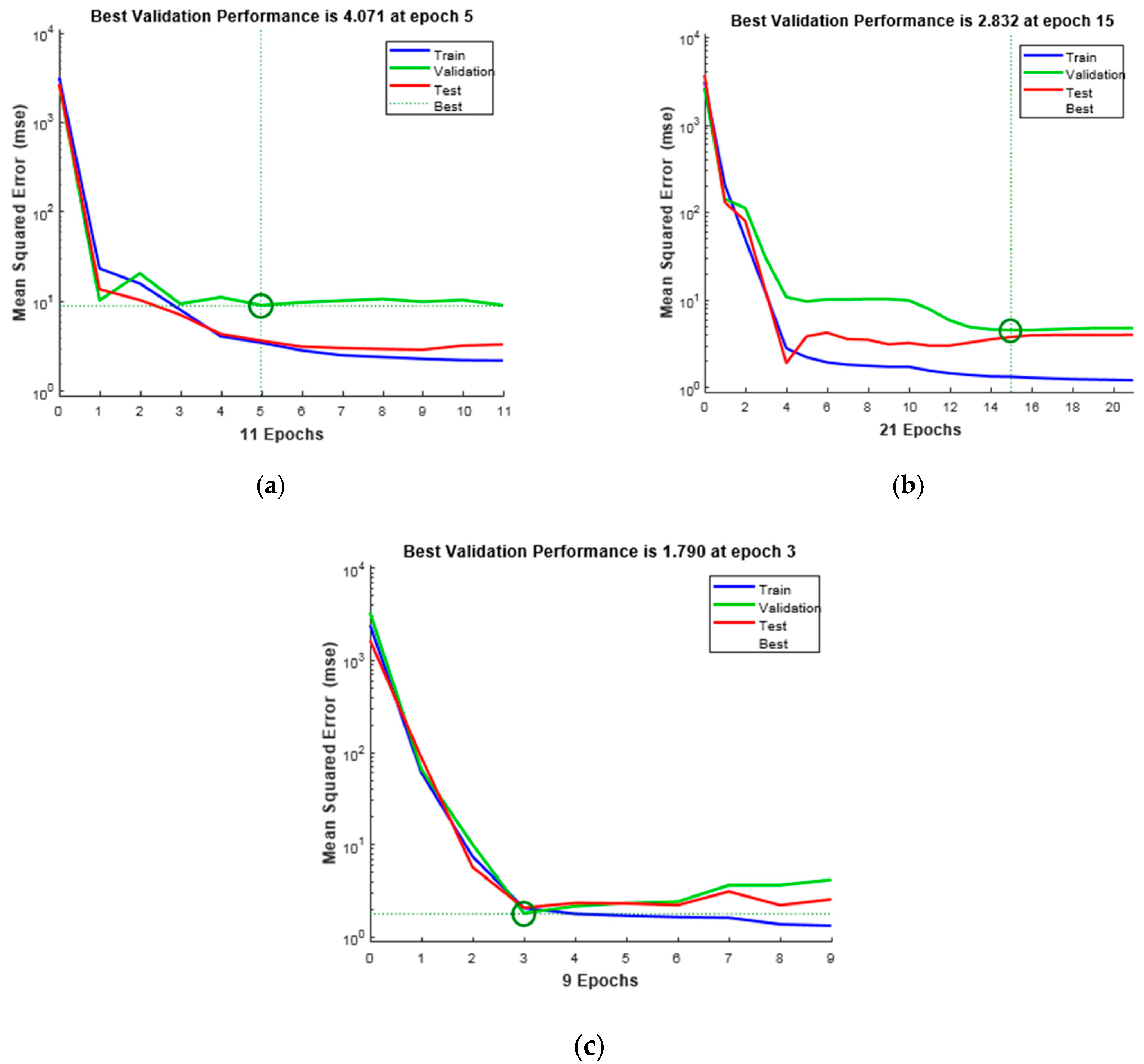
| MSE | 3.864 | 2.404 | 1.719 | 4.071 | 2.832 | 1.790 |
© 2019 by the authors. Licensee MDPI, Basel, Switzerland. This article is an open access article distributed under the terms and conditions of the Creative Commons Attribution (CC BY) license (http://creativecommons.org/licenses/by/4.0/).
Share and Cite
Park, J.Y.; Yoon, Y.G.; Oh, T.K. Prediction of Concrete Strength with P-, S-, R-Wave Velocities by Support Vector Machine (SVM) and Artificial Neural Network (ANN). Appl. Sci. 2019, 9, 4053. https://doi.org/10.3390/app9194053
Park JY, Yoon YG, Oh TK. Prediction of Concrete Strength with P-, S-, R-Wave Velocities by Support Vector Machine (SVM) and Artificial Neural Network (ANN). Applied Sciences. 2019; 9(19):4053. https://doi.org/10.3390/app9194053
Chicago/Turabian StylePark, Jong Yil, Young Geun Yoon, and Tae Keun Oh. 2019. "Prediction of Concrete Strength with P-, S-, R-Wave Velocities by Support Vector Machine (SVM) and Artificial Neural Network (ANN)" Applied Sciences 9, no. 19: 4053. https://doi.org/10.3390/app9194053
APA StylePark, J. Y., Yoon, Y. G., & Oh, T. K. (2019). Prediction of Concrete Strength with P-, S-, R-Wave Velocities by Support Vector Machine (SVM) and Artificial Neural Network (ANN). Applied Sciences, 9(19), 4053. https://doi.org/10.3390/app9194053