Control Technology of Ground-Based Laser Communication Servo Turntable via a Novel Digital Sliding Mode Controller

Abstract

In this study, a sliding mode control (SMC) algorithm was proposed based on a novel reaching law to solve the nonlinear disturbance problem of a ground-based laser communication turntable. This algorithm is a chatter-free method, in which the coefficient of sliding mode variable structure function is designed as an adaptive function, so the chattering of the sliding mode approaches zero. For any perturbed system, this algorithm can ensure a finite time for the system state to reach the sliding mode surface from any initial state. Additionally, the system will stabilize in the quasi-sliding mode domain (QSMD) with O(T³) width, where a narrower QSMD width corresponds to stronger robustness toward nonlinear disturbances. Both mathematical calculations and simulations verified the sliding mode and stability of this control algorithm. Experimental results of the velocity closed-loop of pitch axis show that the proposed algorithm effectively improved the anti-nonlinear disturbance ability of the control system compared with the effects of the traditional digital PID and the existing chatter-reduced SMC algorithms, for smooth system operation.

1. Introduction

Ground-based laser communication is the communication between two or more terminals on the ground, using the atmosphere as the medium and a laser beam as the carrier. Compared with the traditional microwave communication, laser communication offers advantages of low power consumption, high bandwidth, and strong anti-jamming ability, making development of this technology an important focus in the field of information and communication technology [1,2,3].

The communication distance between ground-based laser communication terminals can be extensive, the divergence angle of a laser beam is quite small, and the laser can also be affected by atmospheric turbulence, presenting several challenges to this technology [4,5]. Therefore, to meet the power requirements of laser communication, the servo control system requires micro-radian optical axis alignment accuracy. Currently, coarse and fine two-stage tracking technology is used in most ground-based laser communication systems to ensure alignment accuracy [6,7,8]. Objectively, the coarse tracking control system is the most important part of the control strategy, allowing the isolation of external disturbances to ensure the stability of the optical axis, and the control accuracy determines if the optical axis can be coupled into the fine tracking field of view required for a fine tracking control strategy. A servo turntable is selected here as the actuator, with nonlinear factors such as unbalanced internal torque, friction, torque ripple, model identification error of the control system, and parameter changes, which can lead to unstable operation of the system and restricting system accuracy. Traditional linear control technologies such as use of a digital proportion-integral-differential controller (PID) and lead-lag compensation are unable to meet the accuracy requirements of a coarse tracking system, therefore, a high precision and strong robustness control technology is required to restrain the influence of nonlinear factors on the system and ensure smooth operation of the servo turntable [4].

Several methods have been proposed to suppress the nonlinear disturbance and improve system accuracy, which can be divided into three main approaches. First, the control algorithm structure and the dynamic performance of the control system can be improved by adding a current loop [9], or feedforward compensators [10,11]. Second, the traditional control algorithm can be improved by the incorporation of aspects of modern algorithms, such as fuzzy control [12,13,14] or adaptive control [15,16], which can be applied to improve the robustness of traditional algorithms. Improved algorithms can restrain the influence of nonlinear disturbance on the system, but this approach cannot overcome all the shortcomings of traditional algorithms. Third, the design of a nonlinear controller based on the modern control algorithms, such as active disturbance rejection [17,18], adaptive [19,20], and predictive [11,21] control strategies can avoid the shortcomings of traditional algorithms, effectively compensate for nonlinear disturbances in the system, and improve the accuracy and stability of the system.

Siding mode control (SMC) is an effective approach for a robust control algorithm, and can effectively suppress the nonlinear disturbance of a system. This anti-disturbance control algorithm can ensure that the system state reaches the sliding surface in a finite time and is stable in the quasi-sliding mode domain (QSMD). Once the system state stabilizes at the QSMD, the system state is invariant to system parameter variations and other nonlinear disturbances such as friction [21]. The narrower the QSMD width, the stronger the system robustness to nonlinear disturbances [22]. However, the direct application of the SMC algorithm to ground-based laser communication servo turntable has been a challenge. Large and high frequency chattering of the controller is caused by the switching function in the traditional SMC algorithm, which affect the overall accuracy and stability of the system, and may lead to damage of experimental equipment [23]. Therefore, improving the traditional SMC algorithm to avoid sliding mode chattering is critical for the effective application of SMC algorithm in specific projects.

Several algorithms have been proposed to improve the sliding mode control. The terminal sliding mode algorithm improves the sliding mode surface function design method, and eliminates sliding mode chattering of the controller output by design of a nonlinear sliding mode surface [24,25,26,27]. A higher-order SMC algorithm is applied to extend the design method of traditional SMC output, which eliminates the sliding mode chattering by application of discontinuous control variables to the higher derivatives of sliding mode functions [28]. A robust adaptive second-order SMC was tested to address the tracking problem of uncertain linear systems with both matched and unmatched disturbances, and the results showed that the chattering was removed by applying the sign function for the time-derivative of the control signal [29]. A global SMC was applied to an uncertain chaotic system, and resulted in robustness to multiple delays, parametric uncertainties, and other nonlinear disturbances [30]. A composite nonlinear feedback technique based on a self-tuning integral SMC algorithm was proposed for the robust tracking control of switched systems with uncertainties and input saturation; this technique guaranteed robustness against uncertainties, removed reaching phase, and avoided the chattering problem of sliding mode [31]. A novel adaptive super-twisting-based global-SMC algorithm was proposed to remove the reaching interval and confer robustness and stability to underactuated systems; chatter-free operation was guaranteed by integration of the discontinuous sign function in the control signal [32]. Of these methods, the reaching law function directly defines the approaching movement and sliding mode, making it the most direct, effective, and simple method among the described improved sliding mode algorithms. In this work, a novel chatter-free reaching law algorithm with a disturbance compensation based on the exponential reaching law is proposed for the application in a ground-based laser communication rough tracking control system. This algorithm guarantees that the sliding mode chattering approaches zero and the system state is stabilized in the QSMD with O(T³) (T is the sampling period) width, resulting in superior control that is robust to nonlinear disturbances and model parameter variations.

The main findings of this work can be summarized as follows:

(1)

The frequency domain characteristic of the turntable pitch axis is tested by the classical sweep method [33]. According to the frequency domain characteristic curve, the system model is obtained by the traditional identification method, which is the precondition for the design of SMC.

(2)

A novel reaching law with a disturbance compensator is proposed to solve the chattering problem, which is robust to system model identification error, friction, and other nonlinear disturbances. Both mathematical calculation and simulation support the effectiveness of the algorithm.

(3)

The proposed digital SMC algorithm, the traditional digital PID algorithm, and the existing chatter-reduced SMC algorithm were compared. The experimental results show that the proposed algorithm provides higher control accuracy, stronger anti-interference ability, better frequency domain characteristics, and also suppresses chattering for an improved ground-based laser communication servo turntable control system.

2. Model Identification of Ground-Based Laser Communication Servo Turntable

2.1. System Frequency Domain Characteristic Test

The azimuth or pitch axis control structure of ground-based laser communication servo turntable is shown in Figure 1. The system is composed of a velocity loop controller, a power amplifier, a torque motor, a circular grating encoder, and other parts.

Traditionally, the sinusoidal sweep method is used to test the frequency domain characteristics of the system. As shown in Figure 1, point A indicates the application of the sinusoidal sweep signal, and the speed record at point B encoder feedback value. The input and output data can be used to obtain the system frequency characteristic curve, and the measured frequency domain characteristics include the power amplifier, motor, mechanical structure, and encoder components.

The sinusoidal sweep signal is input at point A, and its digital sequence is expressed as:

$$\begin{array}{c}u(k)=A(k)\sin \left[2\pi \omega (k)\right]\\ \omega (k)=f_1\left(1+c\left(k\right)\cdot {\left(k\cdot t\right)}^n\right),c\left(k\right)=\frac{f_2/f_1-1}{(n+1)T^n}\end{array},$$

(1)

where f₁ is the sweep signal starting frequency, f₂ is the sweep signal termination frequency, t is the sampling time, n is the order of the sweep signal, and T is the sweep signal duration.

Considering the pitch axis of ground-based laser communication servo turntable as an example, a frequency sweep experiment was carried out. During the experiment, the frequency range of sinusoidal sweep signal [f₁, f₂] was set to [0.5, 200], the signal amplitude A(t) was set to 10°/s, the sweep duration T was set to 25 s, and the signal sweep order n was set to the third to ensure sufficient low-frequency data. The sweep input signal and system response curve are shown in Figure 2.

According to the input and output data, the open-loop transmission Bode diagram of the system can be obtained by discrete Fourier transform and power spectrum estimation, as shown in Figure 3. The following conclusions can be drawn explicitly: the turntable pitch axis tends to be linear in the low and middle frequency bands, but there are many nonlinear factors in the system because of the friction of the axis and other factors. There are multi-order resonance links in the high frequency band, and the third-order locked rotor frequency at 105 Hz and the resonant frequency at 113.3 Hz are the main frequencies that affect the system performance. The mechanical structure cannot achieve absolute rigid connection, because of torque imbalance and other nonlinear factors, but the numerical difference between the locked rotor frequency and the resonant frequency is small resulting in strong stiffness.

Remark 1.

It is worth noting that the inverse tangent function is adopted for phase calculation in this method. If the phase difference is less than 90°, the angle value will jump, so ± n180° (n = 1, 2…) should be applied according to the phase angle data value.

2.2. System Model Identification

For practical engineering application, system model identification utilized the mathematical method of medium-low frequency linear fitting and high-frequency two-order model fitting. The essence of this method is to consider the middle and low frequency bands of the system as an ideal linear model and then a polynomial mathematical model is adopted to fit the frequency characteristic curve of the middle and low frequency bands. For the high frequency band, the multi-order resonance frequency in the frequency characteristic curve is fitted by one or more two-order mathematical models. Therefore, the ideal mathematical model of the system can be expressed as follows:

$$G(s)=G_L(s)G_{H_1}(s)G_{H_2}(s)\cdots G_{H_n}(s).$$

(2)

In view of Equation (2), G_L(s) represents the transfer function model of ideal linear link in middle and low frequency band, which is composed of inertial link. G_Hi(s) (i = 1, 2, …, n) represents the transfer function model of the resonance link in high frequency band, which is composed of a two-order mathematical model in series, and its mathematical model is expressed as:

$$G_H(s)=\frac{\frac{1}{{\omega }_z^2}{s}^2+2\frac{{\zeta }_z}{{\omega }_z}s+1}{\frac{1}{{\omega }_p^2}{s}^2+2\frac{{\zeta }_p}{{\omega }_p}s+1}.$$

(3)

The transfer function shown in Equation (3) includes a pair of conjugate complex zero and a pair of complex poles. The complex zeros correspond to systems of high frequency locked rotor frequency ω_z and damping coefficient ζ_z. The double pole corresponds to the resonance frequency ω_p and the damping coefficient ζ_p.

According to the frequency characteristic curve of the pitch axis as shown in Figure 3, the linear transfer function of the middle and low frequency band system can be obtained by the polynomial fitting method as follows:

$$G_L(s)=\frac{3.5}{0.264s+1}.$$

(4)

Shown in the frequency characteristic curve, the third-order resonance mode can have the greatest influence on the high frequency band, and the other modes can be ignored. Therefore, only a second-order mathematical model is sufficient to fit the high-frequency characteristic curve. The high frequency mathematical model is expressed as:

$$G_{H_1}\left(s\right)=\frac{{\left(0.0095s\right)}^2+0.00054s+1}{{\left(0.0088s\right)}^2+0.00066s+1}.$$

(5)

In conclusion, the system model is expressed by the transfer function as:

$$G\left(s\right)=G_L\left(s\right)\cdot G_{H_1}\left(s\right).$$

(6)

The continuous time equation of state corresponds to the transfer function as shown in Equation (6) and can be expressed as:

$$\{\begin{array}{l}\dot{x}\left(t\right)=Ax\left(t\right)+Bu\left(t\right)\\ y\left(t\right)=Cx\left(t\right)\end{array},$$

(7)

where x(t) ϵ R^n×1 is the state vector, y(t) ϵ R^n×1 is the output vector, and A ϵ R^n×n, B ϵ R^n×n, and C ϵ R^1×n are system model parameter matrices. Therefore, according to Equations (5) and (6), the parameter matrixes in Equation (7) can be specifically expressed as follows:

$$\begin{array}{l}A={10}^4\times \left[\begin{array}{ccc}-0.0012& -1.295& -4.89\\ 0.0001& 0& 0\\ 0& 0.0001& 0\end{array}\right],B=\left[\begin{array}{c}1\\ 0\\ 0\end{array}\right]\\ C={10}^5\times \left[\begin{array}{ccc}0.0002& 0.0009& 1.7123\end{array}\right]\end{array}.$$

The characteristic of the open loop frequency domain of the mathematical model shown in Equation (7) has been tested. Given the data presented in Figure 3, the frequency characteristic fitting curve of model identification was constructed and is shown in Figure 4 and the model identification error frequency characteristic curve is presented in Figure 5.

According to the comparison curve of frequency characteristics, the following conclusions can be drawn. The frequency is less than 2 Hz, and the motor is in the running start stage. There is an effect of the static friction force, and the running state is unstable, with obvious amplitude-frequency characteristic curve fluctuation and phase-frequency hysteresis characteristics. The frequency is greater than 2 Hz, and the model frequency characteristic curve can better fit the trend of the actual frequency characteristic curve, however nonlinear disturbances such as friction force and torque imbalance in the system can significantly affect the identification accuracy. The absolute value of the amplitude frequency characteristic curve identification error is less than 8.7 dB. For engineering practice, model identification error and nonlinear disturbance restrict dramatic improvement of the control performance, but a traditional PID controller cannot effectively suppress low and medium frequency nonlinear disturbance, so cannot meet the requirements of high control accuracy of ground-based laser communication. Therefore, it is important to develop a high-precision control algorithm that can better suppress the nonlinear disturbance.

3. Design and Simulation of a Velocity Loop Controller Based on Discrete SMC

This section presents a novel discrete SMC algorithm with a disturbance compensator for low-frequency nonlinear disturbances and model identification error.

3.1. Basic Theory of Discrete SMC

3.1.1. System Discrete Time Ideal Equation of State

According to the identification model equation of state shown in Equation (7), the ideal state equation of the system can be expressed as follows:

$$\dot{x}\left(t\right)=Ax\left(t\right)+Bu\left(t\right)+\zeta \left(t\right).$$

(8)

For the digital control system, the sampling frequency is 1 KHz, and the discretized equation of state is expressed as:

$$x\left(k+1\right)=A_{k}x\left(k\right)+B_{k}u\left(k\right)+\zeta \left(k\right),$$

(9)

where A_k = A_o + ∆A(k), B_k = B_o + ∆B(k) are respectively represented as the real state matrix and output matrix of the system. A_o, B_o are nominal parts of A_k and B_k respectively, which can be obtained by Matlab as follows:

$$A_o=\left[\begin{array}{ccc}0.98& -12.87& -48.52\\ 0.001& 0.99& -0.024\\ 0& 0.001& 1\end{array}\right],B_o={10}^3\cdot \left[\begin{array}{c}0.992\\ 0.0005\\ 0\end{array}\right].$$

The modeling error and the parameter variation ∆A(k), ∆B(k) are assumed to be differentiable with respect to temporal series k, and ζ(k) represents nonlinear factors of the system.

Assumption 1.

The uncertainties ∆A(k), ∆B(k), and ζ(k) are bounded and satisfy the “matching” condition that ∆A(k), ∆B(k), and ζ(k) ϵ span{B_k}.

Therefore, ∆A(k), ∆B(k), and ζ(k) must be able to be unified as nonlinear factors for theoretical research [34,35,36,37,38], as follows:

$$\epsilon \left(k\right)=\Delta A\left(k\right)x\left(k\right)+\Delta B\left(k\right)u\left(k\right)+\zeta \left(k\right),$$

(10)

where ζ(k) satisfies ‖ζ(k)‖<ζ_max with ‖∙‖_∞ being the vector infinity norm and ζ_max being an unknown constant.

Therefore, the discrete equation of state shown in Equation (9) can be rewritten as:

$$x\left(k+1\right)=A_{k}x\left(k\right)+B_{k}u\left(k\right)+\epsilon \left(k\right).$$

(11)

3.1.2. Discrete Sliding Mode Function and the Sliding Mode Surface

In this study, the classical sliding mode function was adopted, which is defined as follows:

$$s\left(k\right)=C_{e}e\left(k\right)=C_e\left(x\left(k\right)-R_n\left(k\right)\right),$$

(12)

where C_e = [C_e(1), C_e(2),…, C_e(n−1), 1] is the sliding mode coefficient matrix, and e(k) represents the error matrix between the ideal state and the actual state. Therefore, the sliding mode surface can be defined as:

$$S=\left\{e\left(k\right)|C_{e}e\left(k\right)=0\right\}.$$

(13)

Lemma 1.

The sliding mode coefficient matrix parameters C_e(1),C_e(2),…,C_e(n−1) satisfy the polynomials pⁿ⁻¹ + C_e(n−1)pⁿ⁻²+…+ C_e(2) + C_e(1), and must be Hurwitz polynomials; p is the Laplace operator [35].

3.1.3. The Quasi Sliding Mode Domain

Definition 1.

For the perturbed system, the system will be in a quasi-sliding-mode (QSM) in the ∆ vicinity of the sliding surface, not at the sliding surface. This specified domain where the QSM occurs is called the quasi-sliding-mode domain (QSMD) s_∆, the positive constant ∆ is the QSMD width, and s_∆ is the QSMD [39,40,41],

$$s_{\Delta }=\left\{s\left(k\right)|\left|s\left(k\right)\right|\le \Delta \right\}$$

(14)

The condition in which the system state is stable in the QSMD is defined as:

$$\{\begin{array}{c}-\Delta <s\left(k+1\right)<s\left(k\right),s\left(k\right)>\Delta \\ s\left(k\right)<s\left(k+1\right)<\Delta ,s\left(k\right)<-\Delta \\ \left|s\left(k+1\right)\right|\le \Delta ,\left|s\left(k\right)\right|<\Delta \end{array}.$$

3.2. A Novel Chatter-Free Approach Law Sliding Mode Control Based on Disturbance Compensator

The SMC algorithm is widely applied in control systems because of its simple structure and good dynamic performance. After stabilization of the system states in the QSMD, the SMC is consistent with the nonlinear disturbance, and the smaller the width of the QSMD, the stronger the robustness of the system to the nonlinear factors. However, chattering is the main problem of SMC, which can lead to high frequency noise in the system, with adverse effects on the stability and control accuracy of the system. In this section, a novel chatter-free SMC algorithm is proposed to reduce the effects of chattering on the system and to suppress nonlinear disturbances in the low and medium frequency bands of the system.

The novel chatter-free sliding mode approach law based on exponential approach law is shown as follows:

$$\{\begin{array}{l}s\left(k+1\right)=\left(1-\lambda T\right)s\left(k\right)-\kappa T\cdot \eta \left(k\right)\cdot \mathrm{sgn}\left[s\left(k\right)\right]+\omega \left(k\right)\\ \eta \left(k\right)=\frac{{\left|e_1\left(k\right)\right|}^{\alpha }}{\delta +\left(1+{\left|e_1\left(k\right)\right|}^{{\alpha }^{-1}}-\delta \right)e^{-\mu \cdot {\left|s\left(k\right)\right|}^{\gamma }}}\end{array},$$

(15)

in this formula, κ > 0 is the coefficient of variable structure function; T is the sampling time of the system; η(k) is the error-related adaptive function, where 0 < δ < 1, γ > 1, μ > 0; |e₁(k)| represents the first state error of the state error vector, if |e₁(k)| > 1, 0 < α<1,if 0 < |e₁(k)| ≤ 1, α > 1; ω(k) represents the disturbance compensator, which can be expressed as:

$$\omega \left(k\right)=C_e\left(\epsilon \left(k\right)-2\epsilon \left(k-1\right)+\epsilon \left(k-2\right)\right).$$

(16)

Remark 2.

If the system state is far away from the sliding mode surface, according to formula (12), s(k) and |e₁(k)| tend to be great, so the coefficient of the switching function sgn[s(k)] tends to be κT∙|e₁|^α/δ, which is greater than κT. The approaching movement is the state of the system that gradually approaches the sliding mode surface driven by the reaching law. If the system state is near the sliding surface, s(k) ≈ 0, and the coefficient of the switching function sgn[s(k)] tends to κT∙|e₁|^α/(1+|e₁|^α), which is far smaller than κT, so the system state is stable in the QSMD for sliding mode motion. Thus, chattering on the sliding surface is reduced.

Lemma 2.

According to [22,42], ε(k) = O(T), ε(k) − ε(k−1) = O(T²), (T is the sampling period), where O(T), and O(T²) represent the disturbance estimation error and are the first-order O(T) and the second-order O(T), respectively; O(T) > O(T²). Therefore, the magnitude of the disturbance estimation error shown in Equation (16) is the third-order O(T), ε(k) − 2ε(k−1) + ε(k−2) = O(T³), O(T³) < O(T²).

According to Equation (11), (12), (15), and (16), the sliding mode controller can be deduced as follows:

$$\begin{array}{c}u(k)={(C_e{B}_k)}^{-1}[C_e(R_n(k+1)-A_{k}x(k))+(1-\lambda T)s(k)\\ -\kappa T\cdot \eta (k)\mathrm{sgn}[s(k)]-C_e(2\epsilon (k-1)-\epsilon (k-2))]\end{array}$$

(17)

Remark 3.

The disturbance function ε(k−1) of the sliding mode controller (17) is usually deduced or calculated by the “time delay estimation method” [22,39,42,43,44]:

$$\epsilon \left(k-1\right)=x\left(k\right)-A_{k}x\left(k-1\right)-B_{k}u\left(k-1\right).$$

(18)

Remark 4.

According to Lemma 2, the width of the QSMD of the proposed SMC is related to the disturbance compensator, and its width is O(T³) order, which is smaller than the O(T²) order width described in [23,42,45]. Therefore, the proposed algorithm attains stronger robustness and higher control accuracy.

3.3. Proof of Robustness and Stability of SMC

Theorem 1.

The absolute value of the system’s nonlinear function equation as shown in Equation (16) has an upper bound, and this upper bound is assumed as ω. The trajectories of the system from any initial state must arrive at the sliding mode surface driven by the proposed algorithm.

Proof. 

There must be an initial state such that the sign of the sliding mode switching functions s(0), s(1), … s(n) does not change, where n is a positive integer. The following proofs are discussed for two cases: s(0) < 0 and s(0) ≥ 0.

1. If s(k) ≥ 0 (k = 0, 1,…n)

Assuming that the system does not cross the sliding surface within the n step, recursive formulas can be obtained according to formula (15).

$$\begin{array}{l}s\left(1\right)=\left(1-\lambda T\right)s\left(0\right)-\left(\kappa T\cdot \eta \left(0\right)+\omega \left(0\right)\right)\\ s\left(2\right)={\left(1-\lambda T\right)}^{2}s\left(0\right)-\left(1-\lambda T\right)\left(\kappa T\cdot \eta \left(0\right)-\omega \left(0\right)\right)-\kappa T\cdot \eta \left(1\right)-\omega \left(1\right)\\ ⋮\\ s\left(n\right)={\left(1-\lambda T\right)}^{n}s\left(0\right)-{\displaystyle \sum _{i=0}^{n-1}{\left(1-\lambda T\right)}^{n-1-i}\left(\kappa T\cdot \eta \left(i\right)-\omega \left(i\right)\right)}\end{array}$$

(19)

There must be a positive number δ so that the following formula is workable:

$${\displaystyle \sum _{i=0}^{n-1}{\left(1-\lambda T\right)}^{n-1-i}\left(\kappa T\cdot \eta \left(i\right)-\omega \left(i\right)\right)}={\displaystyle \sum _{i=0}^{n-1}{\left(1-\lambda T\right)}^{n-1-i}\delta }.$$

(20)

Assuming that the system trajectory reaches the sliding mode surface at time m, then s(m) = 0, and according to Equations (19) and (20), the following equation can be obtained,

$$s\left(m\right)={\left(1-\lambda T\right)}^{m}s\left(0\right)-\delta \cdot {\displaystyle \sum _{i=0}^{m-1}{\left(1-\lambda T\right)}^{m-1-i}}={\left(1-\lambda T\right)}^{m}s\left(0\right)-\delta \frac{1-{\left(1-\lambda T\right)}^m}{\lambda T}$$

(21)

Therefore, the arrival time m can be expressed as:

$$m={\log }_{1-\lambda T}\frac{1}{\lambda T\cdot s\left(0\right)/\delta +1}.$$

(22)

2. Similarly, if s(k) < 0 (k = 0, 1, … n), the moment that the system state reaches the sliding mode surface can be expressed as:

$$m={\log }_{1-\lambda T}\frac{1}{-\lambda T\cdot s\left(0\right)/\delta +1}.$$

(23)

Above all, driven by the sliding mode controller shown in formula (17), the state trajectory of the system from any initial position can reach the sliding mode surface in a limited time, and the arrival time is expressed as follows:

$$m={\log }_{1-\lambda T}\frac{1}{\lambda T\cdot \left|s\left(0\right)\right|/\delta +1}.$$

(24)

Theorem 1 has been proved. □

Theorem 2.

Driven by the sliding mode controller, once the system state reaches the sliding mode surface, it will be stable in the QSMD and cannot escape, the control system is bounded. The QSMD can be expressed as:

$$\Phi =\left\{s\left(k\right)|\left|s\left(k\right)\right|\le \Delta =\kappa T\cdot \eta +\omega \right\},$$

(25)

where ω/κT ≤ η < 1, ω is the upper of the disturbance.

Proof. 

The proof process can be divided into two cases: s(0) < 0 and s(k) ≥ 0 (k = 0, 1,…n).

1. If s(k) ≥ 0 (k = 0, 1,…n), it can be obtained that

$$\begin{array}{c}s\left(k+1\right)=\left(1-\lambda T\right)s\left(k\right)-\kappa T\cdot \eta \left(k\right)\mathrm{sgn}\left[s\left(k\right)\right]+\omega \left(k\right)\\ <s\left(k\right)-\kappa T\cdot \eta +\omega <s\left(k\right)\end{array}$$

(26)

Therefore, when s(k) ≥ 0, the value of s(k) decreases successively. Assuming that the system state is in the QSMD at time n, the system state at time n + 1 must be in the QSMD.

2. If s(k) < 0 (k = 0, 1,…n), similar conclusions can be drawn that

$$\begin{array}{c}s\left(k+1\right)=\left(1-\lambda T\right)s\left(k\right)-\kappa T\cdot \eta \left(k\right)\mathrm{sgn}\left[s\left(k\right)\right]+\omega \left(k\right)\\ >s\left(k\right)+\kappa T\cdot \eta +\omega >s\left(k\right)\end{array}$$

(27)

Therefore, when s(k) < 0, the value of s(k) increases successively. When the system state is in the QSMD at time n, the system state at time n + 1 must also be in the QSMD.

Above all, |s(k)| deceases with time. Once the trajectory of the system reaches the sliding surface, the system state will stabilize in the QSMD. At this moment, the system is strongly robust to nonlinear disturbances. Therefore, the control algorithm is stable, and Theorem 2 is proved. □

Remark 5.

In view of [36,44,46,47,48,49], the overestimation and underestimation problems may exist when the state is stable in the QSMD, we will study it in the future work.

3.4. Sliding Mode Simulation

In this section, using the pitch axis system model of the ground-based laser communication servo turntable shown in Equation (11) as the simulation model, the stability of the proposed sliding mode algorithm was analyzed as follows. Assuming that the nonlinear disturbance of the system is ε(k) = [0;0;2.5sin(2kπ) + 0.5], the initial state of the system is [−1;−0.8;0], and the target state is [0;0;0].

According to the discrete state equation of the system, the sliding mode coefficient shown in Equation (12) is a three-order matrix such that C_e = [C_e1,C_e2,1], the parameters should be chosen as [1,2,1] to satisfy lemma 1. The parameters of the sliding mode controller (17) were selected as: λ = 5, δ = 0.15, α = 2, μ = 10, and γ = 2. To assess the proposed algorithm, it was compared to the classical exponential reaching law (28) with a O(T²) disturbance compensator and the chatter-reduced reaching law (29) with the O(T³) disturbance compensator described in Ref. [22]. The exponential function coefficients are the same, with values of λ_c = 5, λ_[22] = 5, and the variable structure function coefficients κ, κ_c, κ_[22] are determined by the disturbance estimation error in the next section. Other coefficients in the algorithm of Ref. [22] were set to δ_[22] = 0.15, μ_[22] = 10, and γ_[22] = 2.

$$s\left(k+1\right)=\left(1-{\lambda }_{c}T\right)s\left(k\right)-{\kappa }_{c}T\cdot \mathrm{sgn}\left[s\left(k\right)\right]+C_e\epsilon \left(k-1\right).$$

(28)

$$\{\begin{array}{l}s\left(k+1\right)=\left(1-{\lambda }_{[22]}T\right){\varphi }_{[22]}\left(k\right)\cdot s\left(k\right)-\frac{{\kappa }_{[22]}T}{{\varphi }_{[22]}\left(k\right)}\mathrm{sgn}\left[s\left(k\right)\right]+C_e\left[\epsilon \left(k\right)-2\epsilon \left(k-1\right)+\epsilon \left(k-2\right)\right]\\ {\varphi }_{[22]}\left(k\right)={\delta }_{[22]}+\left(1-{\delta }_{[22]}\right)e^{-{\mu }_{[22]}{\left|s(k)\right|}^{{\gamma }_{[22]}}}\end{array}.$$

(29)

The comparison curves of disturbance estimation errors between the three algorithms were determined and are shown in Figure 6. The maximum O(T³) amplitude was 0.01 for the algorithm disturbance estimation error curve for both the proposed algorithm and the Ref. [22] algorithm. This value is much smaller than that of the classical exponential reaching law algorithm, which exhibits a maximum O(T²) amplitude of 0.15. Therefore, the variable structure function coefficients κ and κ_[22] of both algorithms are set as 0.012, and the variable structure function coefficient κ_c of the classical algorithm is set as 0.17. According to Theorem 2, utilization of this parameter, larger than the maximum perturbation estimation, can ensure the stability of the sliding mode trajectory in the QSMD.

Figure 7 shows the sliding mode trajectory contrast curves. Three reaching law algorithms can ensure that the system state arrives at the sliding mode surface in a limited time and is stable in the QSMD with a fixed width. Theorems 1 and 2 are proved here. Compared with the traditional exponential reaching law algorithm, the QSMD width of the proposed reaching law algorithm is narrower, ∆_p ≈ 0.038, compared to the QSMD width of the traditional algorithm of ∆_c ≈ 0.31. It should be noted that a smaller QSMD width correlates to stronger robustness of the system to nonlinear disturbances. Compared with the chatter-reduced reaching law algorithm of Ref. [22], chattering in sliding mode can change to be continuous around the sliding surface, and the widths of both algorithms are almost equal. The proposed algorithm obviously eliminates sliding mode chattering and improves the stability of the system without reducing the robustness of the system.

4. Experimental Verification of Control Algorithm

In this study, a velocity closed-loop experiment was performed, based on the servo turntable pitch axis system for ground-based laser communication. The experimental setup is shown in Figure 8. The experimental devices include the pitch axis motor, which is a DC torque motor (J175LYX04, Chengdu Precision Motor Factory, China), and a C01 motor drive module as the power amplifier (Chengdu Precision Motor Factory, China). The angle value of the pitch motor is set using an encoder (RA26BEA115B05F, Renishaw, UK). The digital controller is composed of a DSP (TMS320F2812) and FPGA (Altera EP1C12Q240). The DSP was used to store the control algorithm, which calculated the control and attitude signals. The FPGA was used to receive and transmit command signals to achieve logic control of the circuit.

The experimental structure is shown in Figure 1, and the input speed signals are fixed, sinusoidal, or closed-loop sweep frequency signals for the speed closed-loop performance test. The classical incremental digital PID controller, the chatter-reduced sliding mode controller of Ref. [22], and the proposed discrete sliding mode controller with disturbance compensation algorithm were tested for application as the speed loop controller. The parameters of the incremental PID controller were set as k_p = 0.8 and k_i = 0.16. The variable structure function coefficients of the proposed and Ref. [22] controllers were set to κT = 0.56, and the other parameters were set in accordance with the sliding mode simulation setting.

4.1. Closed-Loop Experiment of Fixed Speed Signal

For the closed-loop experiment of fixed speed signal, the fixed speed signal of 0.1 mrad/s was input into the pitch axis control system of the ground-based laser communication servo turntable. Under the control of the proposed chatter-free sliding mode controller, the Ref. [22] chatter-reduced sliding mode controller, or the incremental digital PID controller, the motor operation was compared, as shown in Figure 9.

Comparison reveals that all three algorithms can guarantee operation of the motor at the target speed of 0.1 mrad/s. However, there are obvious nonlinear noises in the operation curve of the digital PID controller, the maximum absolute speed error of the PID control accuracy is 37.3 μrad/s, with an absolute error root of mean square (RMS) of 8.3 μrad/s and an average absolute error of 6.5 μrad/s. The nonlinear noise was obviously suppressed for both the proposed method and the method described in Ref. [22]. The maximum absolute speed error of the proposed SMC is 6.9 μrad/s, the absolute error RMS is 1.5 μrad/s and the average absolute error is 1.2 μrad/s. These values are much higher than those obtained for classical PID algorithm, and are slightly smaller than that obtained for the Ref. [22] algorithm, which exhibited a maximum error of 8.3 μrad/s, an average error of 2.3 μrad/s, and RMS of 2.9 μrad/s. Therefore, highest control accuracy was obtained for the proposed chattering-free algorithm, with slightly reduced the performance of the chatter-reduced algorithm described in Ref. [22] because of chattering.

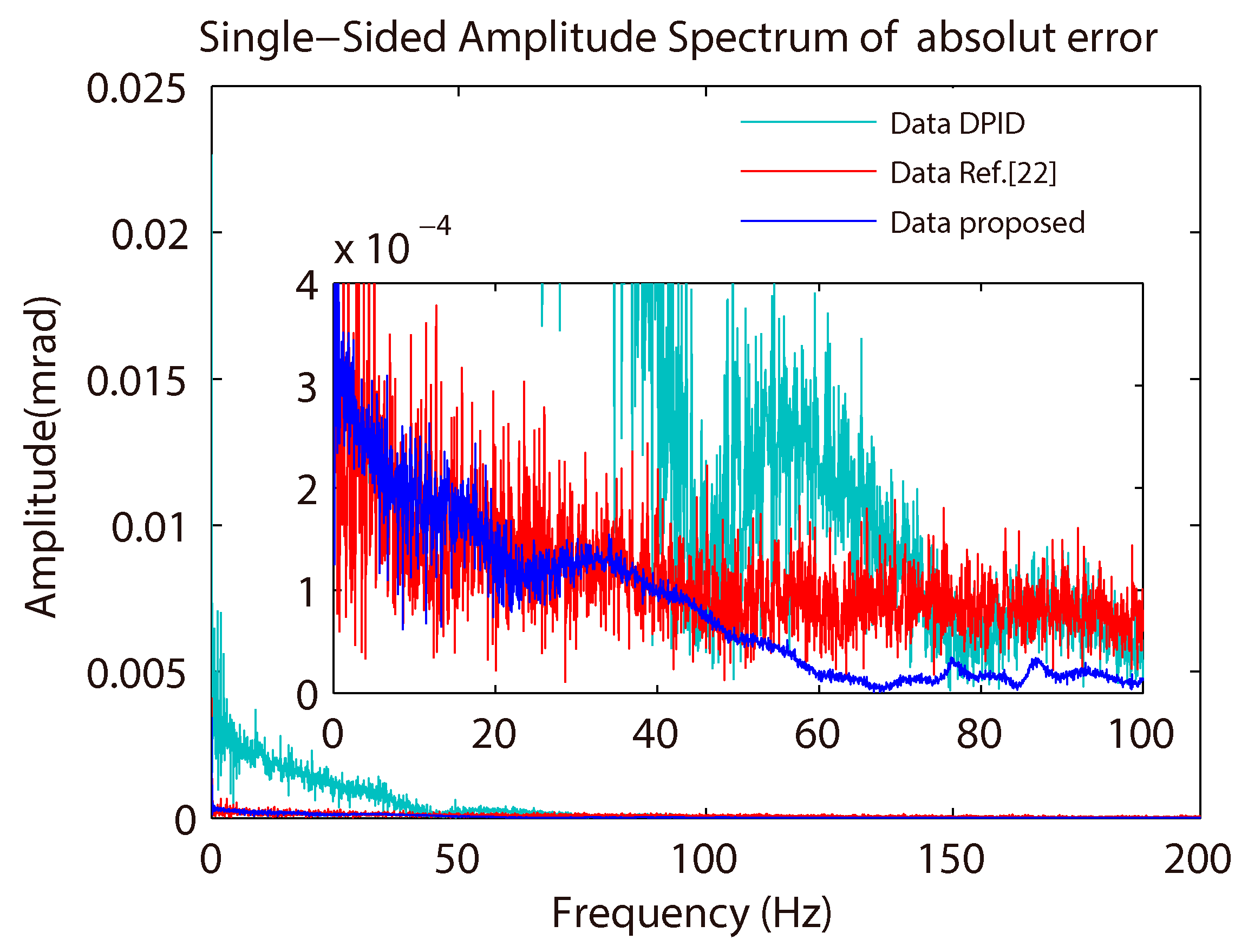
4.2. Sinusoidal Guidance Experiments

For the sinusoidal guidance experiments, the input signal was set to sinusoidal 0.1 mrad/s∙sin(2 Tk), for a sampling time T = 0.001. The velocity sinusoidal guidance contrast curve and sinusoidal guidance error curve are shown as follows.

According to the data presented in Figure 10, the pitch axis motor exhibits smooth sinusoidal operation driven by three controllers, but there are large torque ripples because of nonlinear factors such as friction and nonuniform torque. The data presented in Figure 11 show the absolute value of error. When the servo turntable stably tracks the sinusoidal guidance signal, the absolute error RMS of the PID algorithm is 13.7 μrad/s, the average absolute error is 9.9 μrad/s, and the maximum absolute error is 46 μrad/s. The absolute error RMS of the chatter-reduced algorithm described in Ref. [22] is 2.8 μrad/s, the average absolute error is 2.4 μrad/s, and the maximum absolute error is 15.6 μrad/s. The absolute error RMS of the proposed chatter-free algorithm is 2.3 μrad/s, the average absolute error is 2.1 μrad/s, and the maximum absolute error is 8.1 μrad/s. There is obvious high frequency noise caused by chattering using the algorithm from [22], but this noise is not present when using the proposed chatter-free algorithm. Therefore, to more clearly analyze the frequency distribution of noise, the sinusoidal guidance absolute error was next analyzed by single-sided Fourier transform in the frequency domain, as shown in Figure 12.

According to the results presented in Figure 12, nonlinear disturbance can be effectively suppressed by both the proposed and the algorithm described in [22]. The PID linear controller exhibits limited ability to suppress medium and low frequency noise. There is obvious high frequency noise in the error curve caused by the sliding mode chattering of the Ref. [22] chatter-reduced algorithm, reducing the accuracy and the stability of the system. The high frequency noise is significantly reduced by the proposed chatter-free algorithm.

Meanwhile, it is noted that the biased error generated by the proposed algorithm means that the switching gain is not the optimal, but it is sufficient to prove the advancement of the proposed algorithm. If the switching gain is set to be larger, κT = 0.7, the biased error can be eliminated as shown in Figure 13.

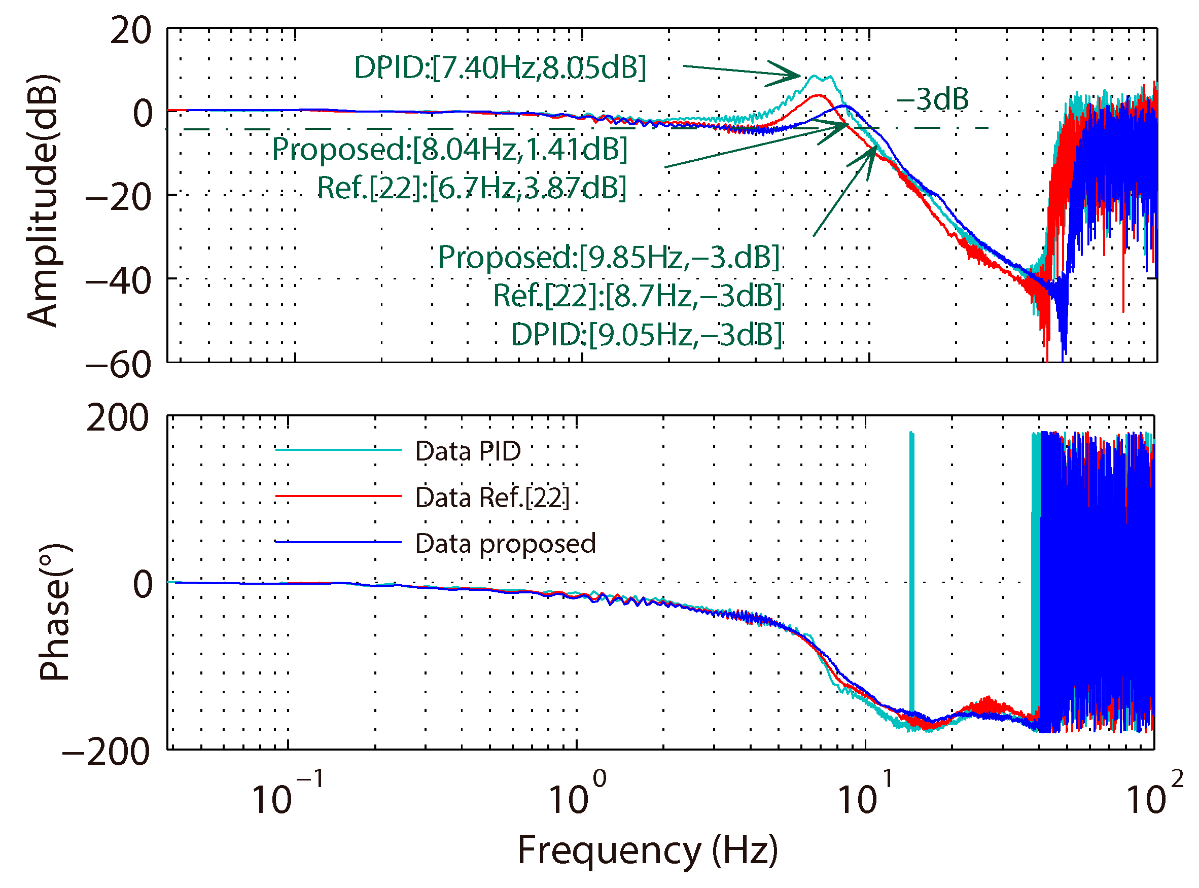
4.3. Closed-Loop Sweep Experiment

In the closed-loop sweep experiment, the input sweep signal was set as shown in Equation (1), the amplitude was set to 1 mrad/s, and the frequency range was set to 0.01 Hz–200 Hz. The closed- loop sweep curve of pitch axis and the frequency characteristic curve of control system are shown in Figure 14 and Figure 15.

According to the frequency characteristic curves shown in Figure 14 and Figure 15, the closed-loop bandwidth of the proposed algorithm is ~9.85 Hz, slightly higher than that of the digital PID, ~9.05 Hz. The closed-loop bandwidth using the Ref. [22] algorithm is the smallest, ~8.7 Hz. Therefore, the dynamic performance of the proposed chatter-free algorithm is much better than that of the previously described chatter-reduced algorithm [22]. The resonance peak of the proposed algorithm is ~1.41 dB, which is much smaller than that of the previous algorithm [22] of ~3.87 dB. The resonance peak of the digital PID is the largest, ~8.05 dB. The smaller the resonance peak is, the better the stability of the system.

4.4. Summary

All results of the three experiments are shown in

Table 1. Summary of experimental results.

Value	Fixed Speed Signal (μrad/s)			Sinusoidal Guidance (μrad/s)			Closed-loop Sweep
Algorithms	RMS	Average	Maximum	RMS	Average	Maximum	Closed-loop Bandwidth	Resonance Peak
PID	8.3	6.5	37.3	13.7	9.9	4.6	9.05Hz	8.05dB
Ref. [22]	2.9	2.3	10.5	2.8	2.4	15.6	8.7Hz	3.87dB
Proposed	1.5	1.2	6.9	2.3	2.1	8.1	9.85Hz	1.41dB

.

5. Conclusion

In this study the pitch axis of the ground-based laser communication servo turntable was considered as the research object, and the frequency domain characteristic of the pitch axis was tested by the sweeping frequency method. Based on the frequency domain characteristic curve, the pitch axis system model was established using a classical model identification method and analyzing the influence of nonlinear disturbance on the system. To address the problems of model identification error and nonlinear disturbance, a novel chatter-free SMC algorithm with a disturbance compensator is proposed. The new algorithm is robust to the system model identification error, friction, and other nonlinear disturbances, and shows good stability by both theoretical calculation and simulation techniques. Finally, the digital PID controller, the chatter-reduced sliding mode controller [22], and the proposed chatter-free sliding mode controller were tested in closed-loop control experiments of pitch axis speed with rated, sinusoidal, or sweep input. The experimental results show that the proposed chatter-free algorithm exhibits higher control accuracy, stronger anti-interference ability, better frequency domain characteristics, and also suppresses chattering for an effective ground-based laser communication servo turntable control system.

The study of the overestimation and underestimation problems of the switching gain when the states are stable in the QSMD will be explored in our future work.

References

1. Jiao, D.D.; Jing, G.; Jie, L.; Xue, D.; Xu, G.J.; Chen, J.P.; Dong, R.F.; Tao, L.; Zhang, S.G. Development and application of communication band narrow linewidth lasers. Acta Phys. Sin. 2015, 64. [Google Scholar] [CrossRef]
2. Mita, T.; Ohashi, J.; Venkatesan, M.; Marma, A.S.P.; Nakamura, M.; Plowe, C.V.; Tanabe, K. Acquisition and tracking control of satellite-borne laser communication systems and simulation of downlink fluctuations. BMC Syst. Biol. 2006, 45, 1–20. [Google Scholar]
3. Smith, R.J.; Casey, W.L.; Begley, D.L. Wideband laser diode transmitter for free-space communication. Opt. Eng. 1988, 27, 344–351. [Google Scholar] [CrossRef]
4. Jian, G.; Yong, A. Design of active disturbance rejection controller for space optical communication coarse tracking system. In Proceedings of the AOPC: Advances in Laser Technology & Applications, Beijing, China, 5–7 May 2015. [Google Scholar]
5. Shimizu, M.; Yamashita, T.; Eto, D.; Toyoshima, M.; Takayama, Y. Cooperative Control Algorithm of the Fine/Coarse Tracking System for 40Gbps Free-Space Optical Communication. In Proceedings of the AIAA International Communications Satellite System Conference, Ottawa, ON, Canada, 24–27 September 2012. [Google Scholar]
6. Kingsbury, R.; Cahoy, K. Development of a pointing, acquisition, and tracking system for a CubeSat optical communication module. In Proceedings of the SPIE LASE, San Francisco, CA, USA, 1–6 February 2015. [Google Scholar]
7. Li, M.Q.; Jiang, S.H. Design of Optimum Controller of APT Fine Tracking Control. System. Adv. Mat. Res. 2013, 712–715, 2738–2741. [Google Scholar] [CrossRef]
8. Min, Z.; Liang, Y. Compound tracking in ATP system for free space optical communication. In Proceedings of the International Conference on Mechatronic Science, Jilin, China, 19–22 Augest 2011. [Google Scholar]
9. Fei, L.; Yan, Z.; Duan, S.; Yin, J.; Liu, B.; Liu, F. Parameter Design of a Two-Current-Loop Controller Used in a Grid-Connected Inverter System With LCL Filter. IEEE Trans. Ind. Electron. 2009, 56, 4483–4491. [Google Scholar]
10. Grzesiak, L.M.; Tarczewski, T. PMSM servo-drive control system with a state feedback and a load torque feedforward compensation. Int. J. Comput. Math. Electric. Electron. Eng. 2013, 32, 364–382. [Google Scholar] [CrossRef]
11. Shen, W.H.; Chen, X.Q.; Pons, M.N.; Corriou, J.P. Model predictive control for wastewater treatment process with feedforward compensation. Chem. Eng. J. 2009, 155, 161–174. [Google Scholar] [CrossRef]
12. Carvajal, J.; Chen, G.; Ogmen, H. Fuzzy PID controller: Design, performance evaluation, and stability analysis. Inf. Sci. 2000, 123, 249–270. [Google Scholar] [CrossRef]
13. Li, H.X.; Zhang, L.; Cai, K.Y.; Chen, G. An improved robust fuzzy-PID controller with optimal fuzzy reasoning. IEEE Trans. Syst. Man Cybern. Part B Cybern. 2005, 35, 1283–1294. [Google Scholar] [CrossRef]
14. Mann, G.I.; Hu, B.G.; Gosine, R.G. Analysis of direct action fuzzy PID controller structures. I IEEE Trans. Syst. Man Cybern. Part B Cybern. 1999, 29, 371–388. [Google Scholar] [CrossRef]
15. Jung, J.W.; Leu, V.Q.; Do, T.D.; Kim, E.K.; Han, H.C. Adaptive PID Speed Control. Design for Permanent Magnet Synchronous Motor Drives. IEEE Trans. Power Electron. 2014, 30, 900–908. [Google Scholar] [CrossRef]
16. Kuc, T.Y.; Han, W.G. An adaptive PID learning control of robot manipulators. Automatica 2000, 36, 717–725. [Google Scholar] [CrossRef]
17. Li, S.; Xu, Y.; Di, Y. Active disturbance rejection control for high pointing accuracy and rotation speed. Automatica 2009, 45, 1854–1860. [Google Scholar] [CrossRef]
18. Zhu, E.; Pang, J.; Na, S.; Gao, H.; Sun, Q.; Chen, Z. Airship horizontal trajectory tracking control based on Active Disturbance Rejection Control. (ADRC). Nonlinear Dyn. 2012, 75, 725–734. [Google Scholar] [CrossRef]
19. Bo, E. Adaptive control stability, convergence, and robustness: Shankar Sastry and Marc Bodson. Automatica 1993, 29, 802–803. [Google Scholar]
20. Liu, Z.G.; Wu, Y.Q. Universal strategies to explicit adaptive control of nonlinear time-delay systems with different structures. Automatica 2018, 89, 151–159. [Google Scholar] [CrossRef]
21. Sun, T.; Pan, Y.; Zhang, J.; Yu, H. Robust model predictive control for constrained continuous-time nonlinear systems. Int. J. Control 2017, 91, 1–16. [Google Scholar] [CrossRef]
22. Ma, H.; Wu, J.; Xiong, Z. A Novel Exponential Reaching Law of Discrete-Time Sliding-Mode Control. IEEE Trans. Ind. Electron. 2017, 64, 3840–3850. [Google Scholar] [CrossRef]
23. Du, H.; Yu, X.; Chen, M.Z.Q.; Li, S. Chattering-free discrete-time sliding mode control. Automatica 2016, 68, 87–91. [Google Scholar] [CrossRef]
24. Abidi, K.; Xu, J.X.; She, J.H. A Discrete-Time Terminal Sliding-Mode Control. Approach Applied to a Motion Control. Problem. IEEE Trans. Ind. Electron. 2009, 56, 3619–3627. [Google Scholar] [CrossRef]
25. Li, S.; Du, H.; Yu, X. Discrete-Time Terminal Sliding Mode Control. Systems Based on Euler’s Discretization. IEEE Trans. Autom. Control 2014, 59, 546–552. [Google Scholar] [CrossRef]
26. Xu, Q. Digital Integral Terminal Sliding Mode Predictive Control. of Piezoelectric-Driven Motion System. IEEE Trans. Ind. Electron. 2016, 63, 3976–3984. [Google Scholar] [CrossRef]
27. Mobayen, S. Adaptive Global Terminal Sliding Mode Control. Scheme with Improved Dynamic Surface for Uncertain Nonlinear Systems. Int. J. Control Autom. Syst. 2018, 16, 1692–1700. [Google Scholar] [CrossRef]
28. Levant, A. Homogeneity approach to high-order sliding mode design. Automatica 2005, 41, 823–830. [Google Scholar] [CrossRef]
29. Mobayen, S.; Tchier, F. A novel robust adaptive second-order sliding mode tracking control technique for uncertain dynamical systems with matched and unmatched disturbances. Int. J. Control Autom. Syst. 2017, 15, 1097–1106. [Google Scholar] [CrossRef]
30. Afshari, M.; Mobayen, S.; Hajmohammadi, R.; Baleanu, D. Global Sliding Mode Control. Via Linear Matrix Inequality Approach for Uncertain Chaotic Systems With Input Nonlinearities and Multiple Delays. J. Comput. Nonlinear Dyn. 2018, 13, 3. [Google Scholar] [CrossRef]
31. Mobayen, S.; Tchier, F. Composite nonlinear feedback integral sliding mode tracker design for uncertain switched systems with input saturation. Commun. Nonlinear Sci. Numer. Simul. 2018, 65, 173–184. [Google Scholar] [CrossRef]
32. Mobayen, S. Adaptive global sliding mode control of underactuated systems using a super-twisting scheme: an experimental study. J. Vib. Control 2019, 25, 2215–2224. [Google Scholar] [CrossRef]
33. Yongting, D.; Hongwen, L.I.; Tao, C. Dynamic analysis of two meters telescope mount control system. Opt. Prec. Eng. 2018, 26, 654–661. [Google Scholar]
34. Kwan, C. Further results on variable output feedback controllers. IEEE Trans. Autom. Control 2001, 46, 1505–1508. [Google Scholar] [CrossRef]
35. Cong, B.L.; Chen, Z.; Liu, X.D. On adaptive sliding mode control without switching gain overestimation. Int. J. Robust Nonlinear Control 2014, 24, 515–531. [Google Scholar] [CrossRef]
36. Roy, S.; Roy, S.B.; Kar, I.N. Adaptive–Robust Control. of Euler–Lagrange Systems With Linearly Parametrizable Uncertainty Bound. IEEE Trans. Control Syst. Technol. 2018, 26, 1842–1850. [Google Scholar] [CrossRef]
37. Huang, Y.J.; Kuo, T.C.; Chang, S.H. Adaptive sliding-mode control for nonlinear systems with uncertain parameters. IEEE Trans. Syst. Man Cybern. B Cybern. 2008, 38, 534–539. [Google Scholar] [CrossRef] [PubMed]
38. Hung, J.Y.; Gao, W.; Hung, J.C. Variable Structure Control: A Survey. IEEE Trans. Ind. Electron. 1993, 40, 21. [Google Scholar] [CrossRef]
39. Ma, H.; Wu, J.; Xiong, Z. Discrete-Time Sliding-Mode Control. with Improved Quasi-Sliding-Mode Domain. IEEE Trans. Ind. Electron. 2016, 63, 6292–6304. [Google Scholar] [CrossRef]
40. Zhang, X.; Sun, L.; Ke, Z.; Li, S. Nonlinear Speed Control. for PMSM System Using Sliding-Mode Control. and Disturbance Compensation Techniques. IEEE Trans. Power Electron. 2013, 28, 1358–1365. [Google Scholar] [CrossRef]
41. Niu, Y.; Ho, D.W.C.; Wang, Z. Improved sliding mode control for discrete-time systems via reaching law. Control Theory Applic. 2010, 4, 2245–2251. [Google Scholar] [CrossRef]
42. Su, W.C.; Drakunov, S.V.; Özgüner, Ü. An O(T2) boundary layer in sliding mode for sampled-data systems. IEEE Trans. Autom. Control 2000, 45, 482–485. [Google Scholar]
43. Morgan, R.Ü.Ö. A decentralized variable structure control algorithm for robotic manipulators. IEEE J. Robot. Autom. 1985, 1, 8. [Google Scholar] [CrossRef]
44. Roy, S.; Lee, J.; Baldi, S. A New Continuous-Time Stability Perspective of Time-Delay Control: Introducing a State-Dependent Upper Bound. Structure. IEEE Control Syst. Lett. 2019, 3, 475–480. [Google Scholar] [CrossRef]
45. Qu, S.; Xia, X.; Zhang, J. Dynamics of Discrete-Time Sliding-Mode-Control. Uncertain Systems With a Disturbance Compensator. IEEE Trans. Ind. Electron. 2014, 61, 3502–3510. [Google Scholar] [CrossRef]
46. Roy, S.; Roy, S.B.; Lee, J.; Baldi, S. Overcoming the Underestimation and Overestimation Problems in Adaptive Sliding Mode Control. IEEE/ASME Trans. Mechatron. 2019. [Google Scholar] [CrossRef]
47. Roy, S.; Roy, S.B.; Kar, I.N. A New Design Methodology of Adaptive Sliding Mode Control for a Class of Nonlinear Systems with State Dependent Uncertainty Bound. In Proceedings of the 15th International Workshop on Variable Structure Systems (VSS), Graz, Austria, 9–11 July 2018. [Google Scholar]
48. Sharma, N.K.; Roy, S.; Janardhanan, S. New design methodology for adaptive switching gain based discrete-time sliding mode control. Int. J. Control 2019. [Google Scholar] [CrossRef]
49. Sharma, N.K.; Roy, S.; Janardhanan, S.; Kar, I.N. Adaptive Discrete-Time Higher Order Sliding Mode. IEEE Trans. Circuits Syst. II Express Br. 2019, 66, 4. [Google Scholar]
Figure 1. Control structure of the pitch axis servo turntable system.
Applsci 09 04051 g001
Figure 2. Input and response signal curve of pitch axis open-loop test.
Applsci 09 04051 g002
Figure 3. Open-loop frequency characteristic curve of pitch axis velocity.
Applsci 09 04051 g003
Figure 4. Frequency characteristic fitting curve of model identification.
Applsci 09 04051 g004
Figure 5. Model identification error frequency characteristic curve.
Applsci 09 04051 g005
Figure 6. Disturbance estimation error contrast curve.
Applsci 09 04051 g006
Figure 7. Sliding mode trajectory contrast curves.
Applsci 09 04051 g007
Figure 8. Ground-based laser communication servo turntable experimental platform: (a) master computer; (b) ground-based laser communication servo turntable; (c) digital controller (power amplifier).
Applsci 09 04051 g008
Figure 9. Contrast curve of rated speed 0.1 mrad/s experiment.
Applsci 09 04051 g009
Figure 10. Velocity sinusoidal guidance contrast curve.
Applsci 09 04051 g010
Figure 11. Absolute value of sinusoidal guidance error curve.
Applsci 09 04051 g011
Figure 12. Frequency domain analysis of guidance absolute error curve.
Applsci 09 04051 g012
Figure 13. Absolute value of sinusoidal guidance error curve.
Applsci 09 04051 g013
Figure 14. Closed-loop sweep curve of pitch axis.
Applsci 09 04051 g014
Figure 15. Contrast curve of the frequency characteristics of the control system.
Applsci 09 04051 g015