Optimal Strokes of Low Reynolds Number Linked-Sphere Swimmers

Abstract

Optimal gait design is important for micro-organisms and micro-robots that propel themselves in a fluid environment in the absence of external force or torque. The simplest models of shape changes are those that comprise a series of linked-spheres that can change their separation and/or their sizes. We examine the dynamics of three existing linked-sphere types of modeling swimmers in low Reynolds number Newtonian fluids using asymptotic analysis, and obtain their optimal swimming strokes by solving the Euler–Lagrange equation using the shooting method. The numerical results reveal that (1) with the minimal 2 degrees of freedom in shape deformations, the model swimmer adopting the mixed shape deformation modes strategy is more efficient than those with a single-mode of shape deformation modes, and (2) the swimming efficiency mostly decreases as the number of spheres increases, indicating that more degrees of freedom in shape deformations might not be a good strategy in optimal gait design in low Reynolds number locomotion.

1. Introduction

Swimming by shape changes at low Reynolds number (LRN) is widely used in biology and micro-robotic design. In this flow regime, inertial effects are negligible, and the micro-organisms or micro-robots propel themselves by exploiting the viscous resistance of the fluid. For example, while a scallop that can only open or close its shell can swim in the ocean by accelerating the surrounding water, such a swimming strategy does not work at LRN, which is generalized by the principle: any time-reversible swimming stroke leads to no net translation at LRN Newtonian fluid, known as the scallop theorem [1].

It is important to understand how the performance of swimming depends on the geometric patterns of shape deformations for micro-swimmers. In microbiology, to fight the viscous resistance, different microorganisms adopt various propulsion mechanisms and directed locomotion strategies for searching for food and running from predators. For example, individual cells such as bacteria find food by a combination of taxis and kinesis using a flagellated or ciliated mode of swimming [2,3,4,5]. Recently, it was discovered that Dd cells can occasionally detach from the substrate and stay completely free in suspension for a few minutes before they slowly sink; during the free suspension stage, cells continue to form pseudopods that convert to rear-ward moving bumps, thereby propelling the cell through the surrounding fluid in a totally adhesion- free fashion [6]. Human neutrophils can swim to a chemoattractant fMLP (formyl-methionylleucyl-phenylalanine) source at a speed similar to that of cells migrating on a glass coverslip under similar conditions [7]. Most recently and equally striking, Drosophila fat body cells can actively swim to wounds in an adhesion-independent motility mode associated with actomyosin-driven, peristaltic cell shape deformations [8]. In micro bio-engineering, medical microrobots revolutionize many aspects of medicine in recent years, which make existing therapeutic and diagnostic procedures less invasive [9]. Different LRN swimming models and micro-robots have been designed since Purcell’s two-hinge model was advanced [1]. In particular, various linked-sphere types of models have appeared, since their simple geometry permits both analytical and computational results [10,11,12,13,14,15,16,17]. These analytical and numerical results have greatly inspired the designs of micro robotic devices, for example, swimmers with 2 and 3 rotatory cylinders have been built to study the hydrodynamic interaction between a wall and an active swimmer [18,19]. Other micro-robots inspired by analytical/numerical works include the Quadroar swimmer, which consists of rotating disks and a linear actuator [20], as well as the Purcell’s two-hinge model [21].

An important problem in LRN swimming is to find the optimized swimming stroke of the micro-swimmer, either (1) with respect to time, i.e., the stroke in one swimming cycle that moves the cell farthest, or (2) with respect to energy, i.e., among all strokes with designated starting and end points, find the one that consumes the least energy. These are usually called the time optimal control and the energy optimal control problems, respectively. Both optimal problems have attracted substantial interest in optimization as well as geometry [22,23,24,25,26,27,28,29,30,31,32,33]. Moreover, recently techniques from machine learning have been applied to linked-sphere types of model gait design, which allows incorporating environmental influences on the micro-swimmer’s swimming behavior, including noise and a frictional medium [34].

Here by investigating the optimal strokes of a group of linked-sphere types of LRN modeling swimmers, we study the efficiencies of propelling mechanisms at LRN of different types of shape deformations. We start from three linked-sphere swimmers–Najafi-Golestanian (NG) 3-sphere accordion model (Figure 1a) [10,11,12], pushmepullyou (PMPY) 2-sphere model (Figure 1b) [15], and the volume-exchange (VE) 3-sphere model (Figure 1c) [17]. All three models have only 2 degrees of freedom in their shape deformations, which is a minimal requirement that enables the swimmer to propel itself at LRN, according to the scallop theorem [1]. In particular, the shape deformations in the three models can be generalized as body elongation and/or mass transportation, and we investigate the efficiencies of these two shape deformation modes on the swimming performances. Then we generalize our results into a linear chain of spheres. The results are presented as follows: in Section 2 we present a brief introduction of the LRN swimming problem; in Section 3 we review the three existing linked-sphere types of swimmers: NG 3-sphere, PMPY 2-sphere and VE 3-sphere models and discuss their optimization problems in Section 4; finally in Section 5 we discuss the optimization problem of models consisting of a chain of spheres.

2. Swimming at LRN by Shape Changes-the Exterior Problem

The Navier-Stokes equations for an incompressible fluid of density $\rho$, viscosity $\mu$, and velocity $\mathbf{u}$ are

$$\begin{array}{ccc}\hfill \rho {\displaystyle \frac{\partial \mathbf{u}}{\partial t}}+\rho \left(\mathbf{u}·\nabla \right)\mathbf{u}& =& -\nabla p+\mu \Delta \mathbf{u}+{\mathbf{f}}_{\mathrm{ext}}\hfill \\ \hfill \nabla ·\mathbf{u}& =& 0\hfill \end{array}$$

where ${\mathbf{f}}_{\mathrm{ext}}$ is the external force field. Herein we assume that the swimmer is self-propelled and does not rely on any exterior force, and therefore we require that ${\mathbf{f}}_{\mathrm{ext}}=\mathbf{0}$. The Reynolds number based on a characteristic length scale L and speed scale U is $\mathrm{Re}=\rho LU/\mu$, and when converted to dimensionless form and the symbols re-defined, the equations read

$$\begin{array}{ccc}\hfill \mathrm{Re}\left[\mathrm{Sl}{\displaystyle \frac{\partial \mathbf{u}}{\partial t}}+\left(\mathbf{u}·\nabla \right)\mathbf{u}\right]& =& -\nabla p+\Delta \mathbf{u}\hfill \\ \hfill \nabla ·\mathbf{u}& =& 0\hfill \end{array}$$

(1)

Here $\mathrm{Sl}=\omega L/U$ is the Strouhal number and $\omega$ is a characteristic frequency of the shape changes. When $\mathrm{Re}\ll 1$ the convective momentum term in Equation (1) can be neglected, but the time variation requires that $\mathrm{ReSl}=\omega L^2/\nu \ll 1$. When both terms are neglected, which we assume throughout, the flow is governed by the Stokes equations:

$$\begin{array}{c}\hfill \mu \Delta \mathbf{u}-\nabla p=\mathbf{0},\nabla ·\mathbf{u}=0\end{array}$$

(2)

We also consider the propulsion problem in an infinite domain and impose the condition ${\mathbf{u}|}_{\mathbf{x}\to \infty }=\mathbf{0}$ on the velocity field.

In the LRN regime time does not appear explicitly, momentum is assumed to equilibrate instantaneously, and bodies move by exploiting the viscous resistance of the fluid. As a result, time-reversible deformations produce no motion, which is the content of the scallop theorem [1]. For a self-propelled swimmer, there is no net force or torque, and therefore movement is a purely geometric process: the net displacement of a swimmer during a stroke is independent of the rate at which the stroke is executed, as long as the Reynolds and Strouhal numbers remain small enough.

Suppose that a swimmer occupies the closed compact domain $\Omega (t)\subset {\mathbb{R}}^3$, at time t, and let $\partial \Omega (t)$ denote its prescribed time-dependent boundary. A swimming stroke $\gamma$ is specified by a time-dependent sequence of the boundary $\partial \Omega (t)$, and it is cyclic if the initial and final shapes are identical, i.e., $\partial \Omega (0)=\partial \Omega (T)$ where T is the period [35]. The swimmer’s boundary velocity $\mathbf{V}$ relative to fixed coordinates can be written as a part $\mathbf{v}$ that defines the intrinsic shape deformations, and a rigid motion $\mathbf{U}$. If $\mathbf{u}$ denotes the velocity field in the fluid exterior to $\Omega$, then a standard LRN self-propulsion problem is:

Given a cyclic shape deformation $\gamma (t)$ that is specified by $\mathbf{v}$, solve the Stokes equations subject to:

$$\begin{array}{c}\mathrm{Boundary}\mathrm{condition}:\mathbf{u}{|}_{\partial \Omega (t)}{=\mathbf{V}=\mathbf{v}+\mathbf{U},\mathbf{u}|}_{\mathbf{x}\to \infty }=\mathbf{0}\hfill \\ \mathrm{Force}-\mathrm{free}\mathrm{condition}:{\int }_{\partial \Omega (t)}\mathbf{f}=\mathbf{0}\hfill \\ \mathrm{Torque}-\mathrm{free}\mathrm{condition}:{\int }_{\partial \Omega (t)}\mathbf{r}\wedge \mathbf{f}=\mathbf{0}\hfill \end{array}$$

In order to treat general shape changes of a swimmer defined by $\Omega (t)\subset {\mathbb{R}}^3$ with boundary $\partial \Omega (t)$, one must solve the exterior Stokes Equations (2) for $\mathbf{u}$, with a prescribed velocity $\mathbf{v}(t)$ on $\partial \Omega (t)$ and subject to the decay conditions $\mathbf{u}\sim 1/r$ and $p\sim 1/r^2$ as $r\to \infty$. The solution has the representation:

$$\begin{array}{c}\hfill \mathbf{u}(\mathbf{x})=-{\displaystyle \frac{1}{8\pi \mu }}{\int }_{\partial \Omega (t)}\mathbf{G}(\mathbf{x},\mathbf{y})·\mathbf{f}(\mathbf{y})dS(\mathbf{y})+{\displaystyle \frac{1}{8\pi }}{\int }_{\partial \Omega (t)}\mathbf{v}(\mathbf{y})·\mathbf{T}(\mathbf{y},\mathbf{x})·\mathbf{n}dS(\mathbf{y})\end{array}$$

where $\mathbf{G}$ is the free-space Green’s function, $\mathbf{T}$ is the associated third-rank stress tensor, $\mathbf{n}$ is the exterior normal and $\mathbf{f}$ is the force on the boundary [36]. The constraints that the total force and the total torque vanish determine the center-of-mass translational and angular velocities. When $\mathbf{x}\in \partial \Omega (t)$, this is an integral equation for the force distribution on the boundary, the solution of which determines the forces needed to produce the prescribed shape changes.

3. Linked-Sphere LRN Swimmers

To date, various simple linked-sphere models for which both analytical and computational results can be obtained have appeared. In particular, there are three linked-sphere models that are designed to investigate the effects of changing body length vs. mass transportation on LRN swimming behavior. The three models are: the NG 3-sphere accordion model (Figure 1a) [10,11,12], the PMPY 2-sphere model (Figure 1b) [15], and the VE 3-sphere model (Figure 1c) [17].

3.1. Fundamental Solutions for Translating and Radially Deforming Spheres

In either of the three models, shape deformations either come from linking-arm length change (the NG and the PMPY models) or radial deformations of the spheres (the PMPY and the VE models). When a sphere of radius $a(t)$ is pulled through a quiescent fluid with a steady force $\mathbf{f}$ under no-slip conditions at the surfaces, the resulting flow field is given by [37]:

$$\begin{array}{c}\hfill \mathbf{u}(\mathbf{r})=\mathbf{f}·\left(1+{\displaystyle \frac{a^2}{6}}{\nabla }^2\right){\displaystyle \frac{\mathbf{G}(\mathbf{x},{\mathbf{x}}_0)}{8\pi \mu }}={\displaystyle \frac{\mathbf{f}}{8\pi \mu r}}·\left[\mathbf{I}+{\displaystyle \frac{\mathbf{r}\mathbf{r}}{r^2}}+{\displaystyle \frac{a^2}{3r^2}}\left(\mathbf{I}-3{\displaystyle \frac{\mathbf{r}\mathbf{r}}{r^2}}\right)\right]\end{array}$$

(3)

where ${\mathbf{x}}_0$ is the position of the center of the sphere and $\mathbf{r}=\mathbf{x}-{\mathbf{x}}_0$, and the resulting velocity of the sphere is given by Stokes’ law

$$\begin{array}{c}\hfill \mathbf{f}=6\pi \mu a\mathbf{U}\end{array}$$

(4)

A second fundamental solution is the velocity field $\mathbf{u}$ produced by a radially-expanding sphere, which can be generated by a point source at the center ${\mathbf{x}}_0$ of the sphere. The corresponding velocity is [36]:

$$\begin{array}{c}\hfill \mathbf{u}=\dot{a}{\left({\displaystyle \frac{a}{r}}\right)}^2{\displaystyle \frac{\mathbf{r}}{r}}={\displaystyle \frac{\dot{v}}{4\pi r^2}}\widehat{\mathbf{r}}\end{array}$$

(5)

where $v=4\pi a^3/3$ is the volume of the sphere and $\widehat{\mathbf{r}}=\mathbf{r}/r$.

By combining the two fundamental solutions (3) and (5), we obtain the solution of the flow velocity generated by a sphere of radius a, centered at ${\mathbf{x}}_0$, subject to a pulling/pushing force $\mathbf{f}$, and radially deforming at the rate $\dot{a}$:

$$\begin{array}{c}\hfill \mathbf{u}(\mathbf{r};a,\mathbf{f},\dot{a})={\displaystyle \frac{1}{24\pi \mu r}}\left[\left(3+{\displaystyle \frac{a^2}{r^2}}\right)\mathbf{f}+3\left(1-{\displaystyle \frac{a^2}{r^2}}\right)\left(\mathbf{f}·\widehat{\mathbf{r}}\right)\widehat{\mathbf{r}}\right]+\dot{a}{\left({\displaystyle \frac{a}{r}}\right)}^2\widehat{\mathbf{r}}\end{array}$$

Next, the fundamental solution involves the interaction between two spheres. Suppose that at time t the ith ($i=1,2$) sphere has radius $a_i(t)$, centered at ${\mathbf{x}}_i(t)$, subjected to force ${\mathbf{f}}_i(t)$ and with radially deforming rate ${\dot{a}}_i(t)$. In the scenario that the two spheres are far apart, i.e., $a_i/l\ll 1$, where $l=|{\mathbf{x}}_1-{\mathbf{x}}_2|$, the translational velocity of the ith sphere can be obtained by the Reflection Method [37,38,39,40,41,42]:

$$\begin{array}{c}\hfill {\mathbf{U}}_i\sim {\displaystyle \frac{{\mathbf{f}}_i}{6\pi \mu a_i}}+\delta {\mathbf{U}}_i^t\left\{j\right\}+\delta {\mathbf{U}}_i^e\left\{j\right\}+O\left({\displaystyle \frac{1}{l^4}}\right)\end{array}$$

(6)

where $\delta {\mathbf{U}}_i^t$ is due to the translation of the other sphere, which arises from the flow given by Equation (3) and is

$$\begin{array}{c}\hfill \delta {\mathbf{U}}_i^t\left\{j\right\}=\left(1+{\displaystyle \frac{a_i^2}{6}}{\nabla }^2\right)\mathbf{u}(\mathbf{r}){|}_{\mathbf{r}={\mathbf{x}}_i-{\mathbf{x}}_j}={\displaystyle \frac{1}{8\pi \mu l}}\left[\left(1+{\displaystyle \frac{a_i^2+a_j^2}{3l^2}}\right)\mathbf{I}+\left(1-{\displaystyle \frac{a_i^2+a_j^2}{l^2}}\right)\widehat{\mathbf{l}}\widehat{\mathbf{l}}\right]{\mathbf{f}}_j\end{array}$$

(7)

where $\mathbf{l}={\mathbf{x}}_i-{\mathbf{x}}_j$. The velocity $\delta {\mathbf{U}}_i^e$ is resulted from a flow generated by the radial deformation of the other sphere, defined by Equation (5):

$$\begin{array}{c}\hfill \delta {\mathbf{U}}_i^e\left\{j\right\}=\left(1+{\displaystyle \frac{a_i^2}{6}}{\nabla }^2\right)\mathbf{u}(\mathbf{r}){|}_{\mathbf{r}={\mathbf{x}}_i-{\mathbf{x}}_j}={\dot{a}}_j{\left({\displaystyle \frac{a_j}{l}}\right)}^2\widehat{\mathbf{l}}\end{array}$$

(8)

Finally, the power consumption P of a sphere with radius a, dragged by a force $\mathbf{f}$, translating at velocity $\mathbf{U}$ and radially expanding/contacting at a rate of $\dot{a}$ comprises two parts: $P^t=\mathbf{f}·\mathbf{U}$ that results from the drag force on the sphere, and $P^e=16\pi \mu a{\dot{a}}^2$ that results from the radial deforming [15,40]. Therefore the total power expended is:

$$\begin{array}{c}\hfill P=P^t+P^e=\mathbf{f}·\mathbf{U}+16\pi \mu a{\dot{a}}^2\end{array}$$

(9)

3.2. Non-Dimensionalization of the System

Let A, L be the characteristic sphere radius and link-arm length. The reflection method holds in the regime $\epsilon :=A/L\ll 1$. Shape deformations of the linked-sphere models (see Section 3.3, Section 3.4 and Section 3.5) come from the expanding/contracting of the link-arms ($\dot{l}$), or the radial expanding/contracting of the spheres ($\dot{a}$). For the shape deformation scales, we require that $\dot{a}/\dot{l}\sim O(1)$, and $\left|\delta a\right|,\left|\delta l\right|\ll A$, where $\delta a$ and $\delta l$ denote the shape deformations in a and l, respectively.

We non-dimensionalize the radii and rod lengths by A and L:

$$\begin{array}{c}\hfill a^{\ast }(t)={\displaystyle \frac{a(t)}{A}},l^{\ast }(t)={\displaystyle \frac{l(t)}{L}}\end{array}$$

We non-dimensionalize other length scales by A as well, and time by T-the swimming stroke period, thus we obtain:

$$\begin{array}{c}{\mathbf{x}}^{\ast }={\displaystyle \frac{\mathbf{x}}{A}},{\nabla }^{\ast }=A\nabla ,t^{\ast }={\displaystyle \frac{t}{T}},{\mathbf{u}}^{\ast }={\displaystyle \frac{T}{A}}\mathbf{u},{\mathbf{U}}^{\ast }={\displaystyle \frac{T}{A}}\mathbf{U}\hfill \\ {\dot{a}}^{\ast }={\displaystyle \frac{d{a}^{\ast }}{d{t}^{\ast }}}={\displaystyle \frac{T}{A}}\dot{a},{\dot{l}}^{\ast }={\displaystyle \frac{d{l}^{\ast }}{d{t}^{\ast }}}={\displaystyle \frac{T}{A}}\dot{l}\hfill \end{array}$$

We assume that the deformations $\delta a,\delta l$ in a and l are of the same order, both of which are scaled by A, thus

$$\begin{array}{c}\hfill {\dot{a}}^{\ast }=\underset{\delta t\to 0}{lim}{\displaystyle \frac{\delta a}{\delta t}}=\underset{\delta t\to 0}{lim}{\displaystyle \frac{T}{A}}{\displaystyle \frac{\delta a^{\ast }}{\delta t^{\ast }}}={\displaystyle \frac{T}{A}}\dot{a},{\dot{l}}^{\ast }=\underset{\delta t\to 0}{lim}{\displaystyle \frac{\delta l}{\delta t}}=\underset{\delta t\to 0}{lim}{\displaystyle \frac{T}{A}}{\displaystyle \frac{\delta l^{\ast }}{\delta t^{\ast }}}={\displaystyle \frac{T}{A}}\dot{l}\end{array}$$

and we have the approximation:

$$\begin{array}{c}\hfill l^{\ast }(t^{\ast }+\delta t^{\ast })={\displaystyle \frac{l(t+\delta t)}{L}}\sim {\displaystyle \frac{l(t)+\dot{l}(t)\delta t}{L}}=l^{\ast }(t^{\ast })+\epsilon {\dot{l}}^{\ast }(t^{\ast })\delta t^{\ast }\end{array}$$

The drag force $\mathbf{f}$ exerted on a sphere of radius a in a quiescent fluid is related to the sphere velocity $\mathbf{U}$ via Equation (4), which leads to the following scaling for forces:

$$\begin{array}{c}\hfill {\mathbf{f}}^{\ast }={\displaystyle \frac{T}{6\pi \mu A^2}}\mathbf{f}=a^{\ast }{\mathbf{U}}^{\ast }\end{array}$$

Therefore Equations (6)–(8) become:

$$\begin{array}{ccc}\hfill {\mathbf{U}}_i^{\ast }& \sim & {\displaystyle \frac{{\mathbf{f}}_i^{\ast }}{a_i^{\ast }}}+\delta {\mathbf{U}}_i^{t\ast }\left\{j\right\}+\delta {\mathbf{U}}_i^{e\ast }\left\{j\right\}+O({\epsilon }^4)\hfill \\ \hfill \delta {\mathbf{U}}_i^{t\ast }\left\{j\right\}& =& {\displaystyle \frac{3\epsilon }{4l^{\ast }}}\left[\left(1+{\epsilon }^2{\displaystyle \frac{a_i^{\ast 2}+a_j^{\ast 2}}{3l^{\ast 2}}}\right)\mathbf{I}+\left(1-{\epsilon }^2{\displaystyle \frac{a_i^{\ast 2}+a_j^{\ast 2}}{l^{\ast 2}}}\right){\widehat{\mathbf{l}}}^{\ast }{\widehat{\mathbf{l}}}^{\ast }\right]{\mathbf{f}}_j^{\ast }\hfill \\ \hfill \delta {\mathbf{U}}_i^{e\ast }\left\{j\right\}& =& {\epsilon }^2{\dot{a}}_j^{\ast }{\left({\displaystyle \frac{a_j^{\ast }}{l^{\ast }}}\right)}^2{\widehat{\mathbf{l}}}^{\ast }\hfill \end{array}$$

Finally, we non-dimensionalize the power P as

$$\begin{array}{c}\hfill P^{\ast }={\displaystyle \frac{1}{6\pi \mu }}{\displaystyle \frac{T^2}{A^3}}P\end{array}$$

so that while $\mathrm{Power}=\mathrm{Force}·\mathrm{Velocity}$ in dimensional form, after non-dimensionalization we still have $P^{\ast }={\mathbf{f}}^{\ast }·{\mathbf{U}}^{\ast }$. Thus the non-dimensional version of Equation (9) is:

$$\begin{array}{c}\hfill P^{\ast }={\mathbf{f}}^{\ast }·{\mathbf{U}}^{\ast }+{\displaystyle \frac{8}{3}}{a}^{\ast }{\dot{a}}^{\ast 2}\end{array}$$

3.3. NG 3-Sphere Swimmer

The NG swimmer (Figure 1a) consists of three spheres with fixed radii $a_i(i=1,2,3)$ and two linking-arms with adjustable length $l_i(t)(i=1,2)$ [10,11,12]. While the spheres are rigid, the linking-arms can stretch or contract. The geometry of the model is shown in Figure 1a, where the three spheres align along the x-axis, numbered from sphere 1 to 3 from left to right. Let $\mathbf{e}$ be the unit vector pointing in the positive x direction, and we have $\mathbf{e}=({\mathbf{x}}_i-{\mathbf{x}}_j)/\parallel {\mathbf{x}}_i-{\mathbf{x}}_j\parallel$ for any pair of $i,j$ with $i>j$. Thus we have ${\mathbf{f}}_i=f_i\mathbf{e}$ and ${\mathbf{U}}_i=U_i\mathbf{e}$ for $i=1,2,3$. For simplicity, we consider the simple geometry $a_1=a_2=a_3=A$. Assume initial shape $l_1(0)=l_2(0)=L$.

The (non-dimensional) velocity of each sphere is given by:

$$\begin{array}{c}\hfill U_i^{\ast }=f_i^{\ast }+\sum _{j\ne i}\delta U_i^{t\ast }\left\{j\right\}=f_i^{\ast }+\sum _{j\ne i}{\displaystyle \frac{3\epsilon }{2l^{\ast }(i,j)}}\left(1-{\displaystyle \frac{2}{3}}{\epsilon }^2{\displaystyle \frac{1}{l^{\ast 2}(i,j)}}\right)f_j\end{array}$$

where $l^{\ast }(i,j)$ is the scaled distance between spheres i and j. The velocities are related via the following relations:

$$\begin{array}{c}\hfill U_2^{\ast }-U_1^{\ast }={\dot{l}}_1^{\ast },U_3^{\ast }-U_2^{\ast }={\dot{l}}_2^{\ast }\end{array}$$

The system is force-free,

$$\begin{array}{c}\hfill \sum _{i=1}^3{f}_i^{\ast }=0\end{array}$$

ad the velocity and power of the swimmer are:

$$\begin{array}{c}\hfill U^{\ast }={\displaystyle \frac{1}{3}}\sum _{i=1}^3{U}_i^{\ast },P^{\ast }=\sum _{i=1}^3{f}_i^{\ast }{U}_i^{\ast }\end{array}$$

3.4. PMPY 2-Sphere Swimmer

The PMPY swimmer (Figure 1b) consists of two spheres with radii $a_i(t)(i=1,2)$ and one linking-arm with length $l(t)$ [15]. The spheres can expand or contract in the radial direction, and the linking-arm can stretch or contract.

The (non-dimensional) velocity of each sphere is given by:

$$\begin{array}{ccc}\hfill U_i^{\ast }& =& {\displaystyle \frac{f_i^{\ast }}{a_i^{\ast }}}+{\left[\delta U_i^{t\ast }\left\{j\right\}+\delta U_i^{e\ast }\left\{j\right\}\right]}_{j\ne i}\hfill \\ & =& {\displaystyle \frac{f_i^{\ast }}{a_i^{\ast }}}+{\left[{\displaystyle \frac{3\epsilon }{2l^{\ast }}}\left(1-{\displaystyle \frac{1}{3}}{\epsilon }^2{\displaystyle \frac{a_i^{\ast 2}+a_j^{\ast 2}}{l^{\ast 2}}}\right)f_j+{(-1)}^{\mathrm{sign}(i-j)}{\epsilon }^2{\dot{a}}_j^{\ast }{\left({\displaystyle \frac{a_j^{\ast }}{l^{\ast }}}\right)}^2\right]}_{j\ne i}\hfill \end{array}$$

The velocities are related by:

$$\begin{array}{c}\hfill U_2^{\ast }-U_1^{\ast }={\dot{l}}^{\ast }\end{array}$$

and the force-free condition is:

$$\begin{array}{c}\hfill \sum _{i=1}^2{f}_i^{\ast }=0\end{array}$$

Assume initial conditions $a_1(0)=a_2(0)=A$ and $l(0)=L$. There is no mass exchange between the swimmer and surrounding fluid, thus the total volume of the two spheres is conserved:

$$\begin{array}{c}\hfill a_1^{\ast 3}+a_2^{\ast 3}=2,\sum _{i=1}^2{a}_i^{\ast 2}{\dot{a}}_i^{\ast }=0\end{array}$$

The velocity and power of the whole swimmer are:

$$\begin{array}{c}\hfill U^{\ast }={\displaystyle \frac{1}{2}}\sum _{i=1}^2{U}_i^{\ast },P^{\ast }=\sum _{i=1}^2\left(f_i^{\ast }{U}_i^{\ast }+{\displaystyle \frac{8}{3}}{a}_i^{\ast }{\dot{a}}_i^{\ast 2}\right)\end{array}$$

3.5. VE 3-Sphere Swimmer

The VE swimmer (Figure 1c) consists of three spheres with radii $a_i(t)(i=1,2,3)$ and two rigid linking-arms with fixed length $l_i(i=1,2)$ [17]. The spheres can only expand or contract in the radial direction, and each can only exchange mass with its neighboring sphere(s), that is, between sphere 1 and 2, or between sphere 2 and 3, but not between sphere 1 and 3.

The (non-dimensional) velocity of each sphere is given by:

$$\begin{array}{ccc}\hfill U_i^{\ast }& =& {\displaystyle \frac{f_i^{\ast }}{a_i^{\ast }}}+\sum _{j\ne i}\left[\delta U_i^{t\ast }\left\{j\right\}+\delta U_i^{e\ast }\left\{j\right\}\right]\hfill \\ & =& {\displaystyle \frac{f_i^{\ast }}{a_i^{\ast }}}+\sum _{j\ne i}\left[{\displaystyle \frac{3\epsilon }{2l^{\ast }(i,j)}}\left(1-{\displaystyle \frac{1}{3}}{\epsilon }^2{\displaystyle \frac{a_i^{\ast 2}+a_j^{\ast 2}}{l^{\ast 2}(i,j)}}\right)f_j+{(-1)}^{\mathrm{sign}(i-j)}{\epsilon }^2{\dot{a}}_j^{\ast }{\left({\displaystyle \frac{a_j^{\ast }}{l^{\ast }(i,j)}}\right)}^2\right]\hfill \end{array}$$

Assume initial conditions $a_1(0)=a_2(0)=a_3(0)=A$ and $l_1=l_2=L$. The system is force-free and total volume is conserved:

$$\begin{array}{c}\hfill \sum _{i=1}^3{f}_i^{\ast }=0,\sum _{i=1}^3{a}_i^{\ast 3}=3,\sum _{i=1}^3{a}_i^{\ast 2}{\dot{a}}_i^{\ast }=0\end{array}$$

The velocity and power of the whole swimmer are:

$$\begin{array}{c}\hfill U^{\ast }=U_1^{\ast }=U_2^{\ast }=U_3^{\ast },P^{\ast }=\sum _{i=1}^3\left(f_i^{\ast }{U}_i^{\ast }+{\displaystyle \frac{8}{3}}{a}_i^{\ast }{\dot{a}}_i^{\ast 2}\right)\end{array}$$

Notice that the linking-arms are rigid.

4. Optimal Strokes of NG, PMPY and VE Swimmers

4.1. Euler–Lagrange Equation for Optimal Strokes of LRN Swimmers

(Hereafter we will continue our discussion using the non-dimensional quantities but omitting the ∗ notation for simplicity). As is introduced in Section 2, a swimming stroke $\gamma (t)$ is a t-series of swimmer shapes. In the case when the swimmer has only finitely many degrees of freedom in their shape deformations, $\gamma$ can be considered as a function from $[0,T]$ to ${\mathbb{R}}^m$, where m is the number of degrees of freedom of the swimmer, and each component in $\gamma (t)$ defines one degree of freedom. For example, all three linked-sphere swimmers in Section 3.3, Section 3.4 and Section 3.5 have only 2 degrees of freedom, thus we have ${\gamma }_{\mathrm{NG}}(t)={(l_1(t),l_2(t))}^T$ for a NG swimmer, ${\gamma }_{\mathrm{PMPY}}(t)={(l(t),a_1(t))}^T$ for a PMPY swimmer, and ${\gamma }_{\mathrm{VE}}(t)={(a_1(t),a_3(t))}^T$ for a VE swimmer.

The linear and driftless properties of Stokes flows make the LRN swimming problem a classic driftless controllable system [25,28,31,32,35,43,44]. Consider a cyclic stroke $\gamma (t)$ of a LRN swimmer, where $t\in [0,1],\gamma (0)=\gamma (1)$. The net translation $X(\gamma )$ and energy dissipation $\mathcal{E}(\gamma )$ within a stroke can be represented as:

$$\begin{array}{ccc}\hfill X(\gamma )& =& {\int }_0^{1}U(\gamma )dt={\int }_0^1\mathcal{F}(\gamma )·\dot{\gamma }dt\hfill \end{array}$$

(10)

$$\begin{array}{ccc}\hfill \mathcal{E}(\gamma )& =& {\int }_0^{1}P(\gamma )dt={\int }_0^1\left(\mathcal{G}(\gamma )\dot{\gamma },\dot{\gamma }\right)dt\hfill \end{array}$$

(11)

where for NG, PMPY and VE equations, the operators $\mathcal{F}$ and $\mathcal{G}$ can be calculated from the equations from Section 3.3, Section 3.4 and Section 3.5, respectively. For a given initial shape which we denote by ${\gamma }_0$ and a given net translation $X_0$, let $\Gamma \{{\gamma }_0,X_0\}$ be the set of all cyclic strokes that starts and ends with shape ${\gamma }_0$ and results in a net translation of $X_0$ in a cycle:

$$\begin{array}{c}\hfill \Gamma \{{\gamma }_0,X_0\}=\left\{\gamma \right|\gamma (0)=\gamma (1)={\gamma }_0,X(\gamma )=X_0\}\end{array}$$

The optimal stroke problem can be formulated as follows:

Given an initial shape ${\gamma }_0$ and a net translation $X_0$, find the stroke $\overline{\gamma }$ in $\Gamma \{{\gamma }_0,X_0\}$ that minimizes the energy dissipation $\mathcal{E}$:

$$\begin{array}{c}\hfill \mathcal{E}(\overline{\gamma })=\underset{\gamma \in \Gamma \{{\gamma }_0,X_0\}}{min}\mathcal{E}(\gamma )\end{array}$$

(12)

The Euler–Lagrange equation for this optimization problem is [22,23]:

$$\begin{array}{c}\hfill -{\displaystyle \frac{d}{dt}}\left(\mathcal{G}\dot{\gamma }\right)+{\displaystyle \frac{1}{2}}\left(\begin{array}{c}({\partial }_{{\gamma }_1}\mathcal{G}\dot{\gamma },\dot{\gamma })\\ ({\partial }_{{\gamma }_2}\mathcal{G}\dot{\gamma },\dot{\gamma })\\ ⋮\\ ({\partial }_{{\gamma }_m}\mathcal{G}\dot{\gamma },\dot{\gamma })\end{array}\right)+\lambda \left[{(\nabla \mathcal{F})}^T-\nabla \mathcal{F}\right]·\dot{\gamma }=0\end{array}$$

(13)

where m is the number of degrees of freedom in the swimmer’s shape deformation, and $\gamma ={({\gamma }_1,{\gamma }_2,\cdots ,{\gamma }_m)}^T\in {\mathbb{R}}^m$. Solutions of Equation (13) give the geodesics connecting $({\gamma }_0,0)$ and $({\gamma }_0,X_0)$, which we refer to as the geodesic strokes. The optimal stroke is the geodesic stroke that consumes the least energy [22,23].

We use the Shooting Method (SM) to numerically solve the governing Equation (13) for the optimal stroke problem. The numerical methods are developed in [22,23] and have been applied for NG with equal sizes and PMPY swimmers; recent research works also report the efficiency of NG swimmers with unequal sized sphere [45]. In the following we use SM for all three (NG, PMPY and VE) linking-arm swimmers and compare their swimming performances. In Appendix A we present an outline of SM for the convenience of the readers of this paper.

4.2. Numerical Results

The numerical results of optimal strokes of a NG 3-sphere, PMPY 2-sphere and VE 3-sphere swimmers are given in

Table 1. Energy dissipation $\mathcal{E}(\overline{\gamma })$ and efficiency Eff.

$\mathit{X}(\overline{\mathit{\gamma }})$	NG 3-Sphere		PMPY 2-Sphere		VE 3-Sphere
	$\mathcal{E}(\overline{\mathbf{\gamma }})$	Eff	$\mathcal{E}(\overline{\mathbf{\gamma }})$	Eff	$\mathcal{E}(\overline{\mathbf{\gamma }})$	Eff
$0.001$ (Figure 2a,b)	$37.61\times {10}^{-2}$	$2.66\times {10}^{-3}$	$3.37\times {10}^{-2}$	$29.67\times {10}^{-3}$	$95.87$	$1.04\times {10}^{-3}$
$0.005$	$182.96\times {10}^{-2}$	$2.73\times {10}^{-3}$	$16.82\times {10}^{-2}$	$29.73\times {10}^{-3}$	$539.33\times {10}^{-2}$	$0.93\times {10}^{-3}$
$0.01$ (Figure 2c,d)	$358.28\times {10}^{-2}$	$2.79\times {10}^{-3}$	$33.55\times {10}^{-2}$	$29.81\times {10}^{-3}$	-	-
$0.02$	$695.46\times {10}^{-2}$	$2.88\times {10}^{-3}$	$66.77\times {10}^{-2}$	$29.95\times {10}^{-3}$	-	-
$0.05$	$1636.25\times {10}^{-2}$	$3.06\times {10}^{-3}$	$164.91\times {10}^{-2}$	$30.33\times {10}^{-3}$	-	-
$0.1$	-	-	$320.94\times {10}^{-2}$	$31.16\times {10}^{-3}$	-	-
$0.2$	-	-	$606.30\times {10}^{-2}$	$32.99\times {10}^{-3}$	-	-

and Figure 2, where we take $\epsilon =A/L=0.2$ in all simulations. For different values of the net translation X, the optimal strokes $\overline{\gamma }$ of the three swimmers are computed by the SM method described in Section 4.1 and Appendix A, the energy dissipation of the optimal strokes $\mathcal{E}(\overline{\gamma })$ is recorded in Table 1, and the $\gamma$-paths (solid lines) and the $X(\overline{\gamma }(t))$, $t\in [0,1]$ trajectories (dashed lines) are given in Figure 2. The simulation results show that PMPY is the most efficient swimmer among the three, next is NG, the last is VE:

$$\begin{array}{c}\hfill {\mathrm{Eff}}_{\mathrm{PMPY}}>{\mathrm{Eff}}_{\mathrm{NG}}\sim {\mathrm{Eff}}_{\mathrm{VE}}\end{array}$$

where we define the efficiency of an LRN swimmer as the net translation to energy dissipation ratio of the optimal stroke of the swimmer:

$$\begin{array}{c}\hfill \mathrm{Eff}={\displaystyle \frac{X(\overline{\gamma })}{\mathcal{E}(\overline{\gamma })}},\mathrm{where}\overline{\gamma }\mathrm{is}\mathrm{the}\mathrm{optimal}\mathrm{stroke}.\end{array}$$

(14)

The dimensional form of Eff has the unit of force${}^{-1}$. In addition, from Table 1 we find that for single loop optimal strokes, the efficiency for each swimmer is about the same for different values of $X(\overline{\gamma })$, with a slight increase in the efficiency for NG and PMPY swimmers as $X(\overline{\gamma })$ increases:

$$\begin{array}{c}\hfill {\mathrm{Eff}}_{\mathrm{PMPY}}\sim 29.5-33.0\times {10}^{-3},{\mathrm{Eff}}_{\mathrm{NG}}\sim 2.6-3.1\times {10}^{-3},{\mathrm{Eff}}_{\mathrm{VE}}\sim 1\times {10}^{-3}\end{array}$$

As X increases, geodesic strokes of multiple loops show up for NG and PMPY swimmers. However, we do not catch multi-loop solutions in our numerical simulations for VE swimmers, as large shape deformations of VE models easily lead to negative volume of the spheres. Comparing to single loop geodesic strokes, multi-loop geodesic strokes are less efficient (see Appendix B).

We summarize our main conclusions from the above numerical results as follows:

• A PMPY model that adopts a mixed-mode of shape deformations is the most efficient among the three; next is NG and the last is VE, both of which adopt a single-mode of shape deformations (see Remark below).
• Single-loop geodesic strokes are more efficient than multi-loop geodesic strokes.
• The efficiency of a given LRN swimmer is almost the same for different X, as long as the optimal stroke is single-looped.

Finally, we numerically compare the optimal strokes of the three model swimmers to stepwise square strokes. The results are presented in Appendix C, which clearly shows the improvement of swimming efficiency in the optimal strokes comparing to the stepwise square strokes.

Remark 1.

At LRN, different microorganisms adopt various propulsion mechanisms and directed locomotion strategies for searching for food and running from predators. While many microorganisms including bacteria use a flagellated or ciliated mode of swimming [2,3,4,5,46,47,48,49,50,51,52,53], some cells use an amoeboid swimming strategy, which relies on the generation, protrusion and even travel of pseudopodia or blebs [6,7,54]. Such shape deformations propagating over the whole cell body can usually be generalized as a combination of two modes: stretching of the cell body, and mass transportation along the cell body. Comparing with the linked-sphere types of models, cell body stretching can be considered as mode $\dot{l}$ while mass transportation as mode $\dot{a}$. According to the scallop theorem [1], a minimal LRN swimmer has at least two degrees of freedom in its shape deformations, therefor we have three possible combinations: two single-mode of shape changes: both in body stretching (both are $\dot{l}$-type of shape deformations), both in mass transportation (both are $\dot{a}$-type of shape deformations), and a mixed-modes of shape change: body stretching combined with mass transportation $(\dot{l},\dot{a})$. It is clearly seen that the three combinations correspond to the three linked-sphere swimmers (NG, VE and PMPY) we discussed here, and our numerical results indicate that:

Comparing to single-mode shape deformations, mixed-modes of shape deformations, i.e., body stretching combined with mass transportation is more efficient when swimming at LRN.

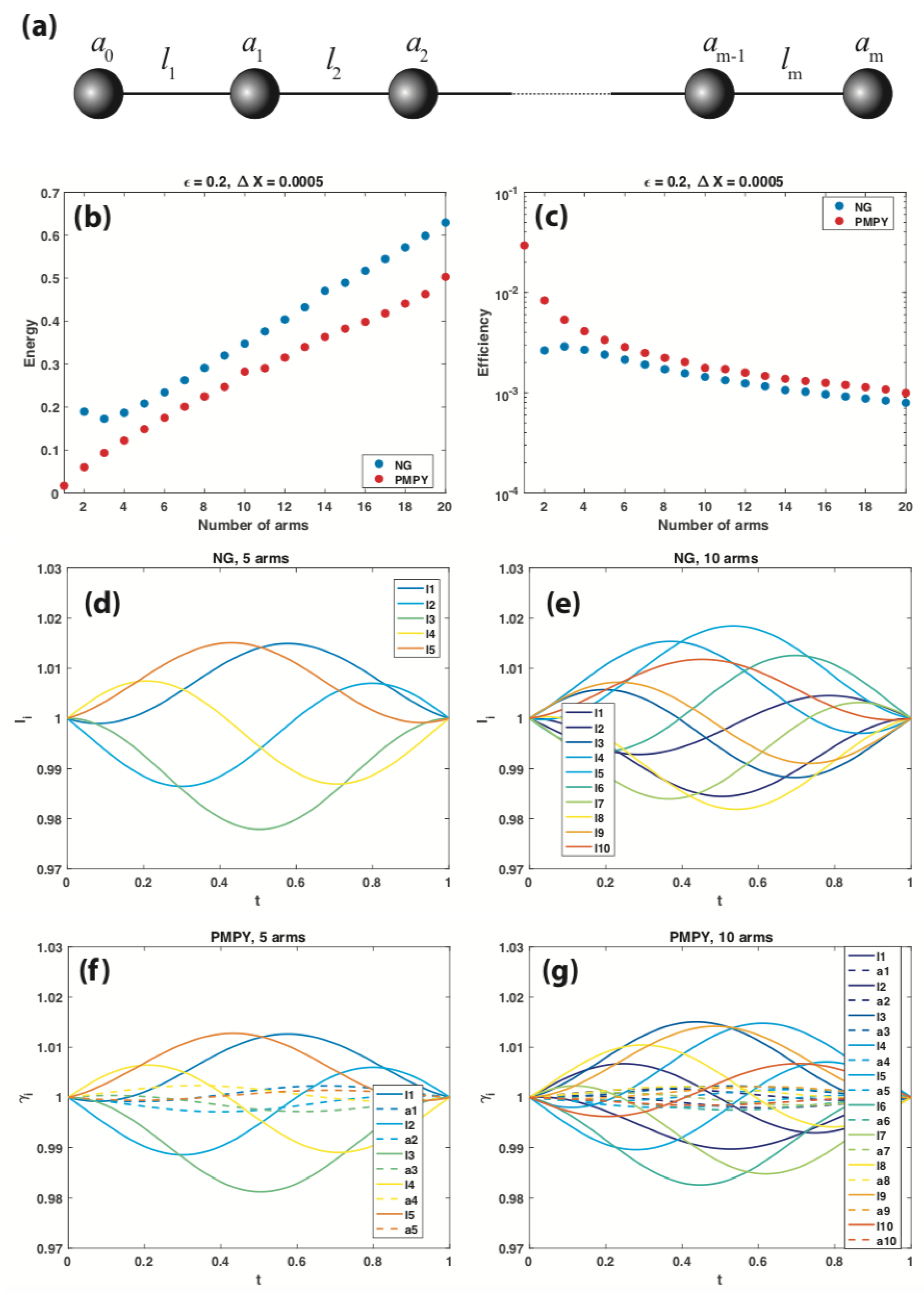
An asymptotic analysis study on the three swimmers that derives the same conclusion can be found in [55], which illustrates that a PMPY swimmer has a net translation $X(\gamma )\sim O(1)$, comparing to $X(\gamma )\sim O({\epsilon }^2)$ for a NG or a VE swimmer. Therefore the mixed control strategy as is adopted by a PMPY swimmer is superior to uni-mode of control strategies as are adopted by a NG or a VE swimmer.

Remark 2.

A more popular definition of efficiency of NG swimmer in its dimensional form is given by [30]:

$$\begin{array}{c}\hfill {\mathrm{Eff}}^{-1}={\displaystyle \frac{\frac{1}{T}{\int }_0^{T}P(\gamma )dt}{6\pi \mu A{X}^2}}\end{array}$$

which measures the ratio of the average energy dissipation in the stroke γ to that applied to a rigid sphere of radius A traveling the same distance X. However, this definition does not apply well to our discussion in that (1) we are considering non-rigid spheres where the spheres are allowed to deform radially, and (2) we are comparing swimmers of different numbers of spheres. Therefore we adopt the definition given by Equation (14) instead.

5. Optimal Strokes of $(\mathit{m}+\mathbf{1})$-Linked-Sphere LRN Swimmers

In this section we will discuss $(m+1)$-linked-sphere LRN swimmers, starting from the NG-type of swimmers (Section 5.1), where rigid spheres are considered and shape deformations are only allowed to be in linking-arms length changes. Next we consider the PMPY-type of swimmers (Section 5.2), where both spheres and linking-arms are allowed to deform. Finally we discuss the effect of sphere separation distance on the swimmer’s swimming efficiency (Section 5.3).

5.1. $(m+1)$-Linked-Sphere NG Swimmers

An $(m+1)$-linked-sphere NG swimmer consists of $m+1$ spheres with fixed radii $a_i(i=0,1,2,\cdots ,m)$ and m linking-arms with adjustable length $l_i(t)(i=1,2,\cdots ,m)$. The geometry of the model is shown in Figure 3a, where the swimmer lies along the x-axis, and the spheres and linking-arms are numbered from left to right. We assume equal-sized spheres $a_0=a_1=\cdots =a_m=A$ and initial shape $l_1(0)=l_2(0)=\cdots =l_m(0)=L$. The equation system describing the mechanics of the model follows that in Section 3.3. We follow the same numerical scheme to solve the optimization problem Equation (12) for different numbers of linking-arms m. In our simulations, we test for $m\in [2,20]$ and with small net translation $X=5\times {10}^{-4}$ and $\epsilon =A/L=0.2$ in all simulations.

The energy dissipation of the optimal stroke reaches a minimum ${min}_m\mathcal{E}(\overline{\gamma })=17.28\times {10}^{-2}$ at $m=3$, i.e., a 4-sphere NG swimmer; after that, $\mathcal{E}(\overline{\gamma })$ increases as m increases (Figure 3b, blue dots). Correspondingly, the most efficient swimmer is the 4-sphere NG swimmer with Eff $=2.89\times {10}^{-3}$, and the efficiency decreases as m increases (Figure 3c, blue dots).

According to the scallop theorem [1], a minimal LRN swimmer should have at least 2 degrees of freedom. When it comes to LRN swimmers with more than 2 degrees of freedom, the question is: is it better to use all degrees of freedom or to take a subset of them so to reach more efficient swimming strategy? In our simulations, we find that the optimal strokes for different numbers of linking-arms have all made use of all degrees of freedom, for example, Figure 3d,e show the $\gamma$-paths of the optimal strokes for 5 and 10 arms, respectively, which show that all linking-arms performed length deformations in the optimal stroke, none is disabled.

5.2. $(m+1)$-Linked-Sphere PMPY Swimmers

Next we consider $(m+1)$-linked-sphere PMPY swimmers, which consist of $m+1$ spheres with adjustable radius $a_i(t)(i=0,1,2,\cdots ,m)$ and m linking-arms with adjustable length $l_i(t)(i=1,2,\cdots ,m)$ (Figure 3a). We assume initial shape $a_0(0)=a_1(0)=\cdots =a_m(0)=A$ and $l_1(0)=l_2(0)=\cdots =l_m(0)=L$. Under the volume conservation constraint of all spheres, we take $a_1,a_2,\cdots ,a_m$ to be controls while $a_0(t)$ can be obtained from the volume conservation constraint. The equation system of the model follows that in Section 3.4. In our simulations, we test for $m\in [1,20]$ and with small net translation $X=5\times {10}^{-4}$ and $\epsilon =A/L=0.2$ in all simulations.

The energy dissipation of the optimal stroke reaches a minimum ${min}_m\mathcal{E}(\overline{\gamma })=1.70\times {10}^{-2}$ at $m=1$, i.e., a 2-sphere PMPY swimmer, which is the one we discussed in Section 3.4. $\mathcal{E}(\overline{\gamma })$ increases as m increases (Figure 3b, red dots). Correspondingly, the most efficient swimmer is the 2-sphere NG swimmer with Eff $=29.5\times {10}^{-3}$, and the efficiency decreases as m increases (Figure 3c, red dots). Comparing to NG type of swimmers with the same structure (i.e., same numbers of spheres and linking-arms), PMPY swimmers consumes less energy and is thus more efficient (Figure 3b,c).

Similar to NG swimmers, for PMPY swimmers, the optimal strokes for different numbers of linking-arms have also made use of all degrees of freedom. Figure 3f,g show the $\gamma$-paths of the optimal strokes for 5 and 10 arms, respectively, which show that all linking-arms performed length deformations and all spheres performed radial deformations in the optimal stroke. In addition, we find that for large m, the amplitude of sphere radial deformations $a_i(t)$ are smaller than that of the linking-arms length changes $l_i(t)$ (Figure 3f,g); on the other hand, in the most efficient PMPY type of swimmers, i.e., the 2-sphere PMPY swimmer, the amplitude of sphere radial deformation $a_1(t)$ is larger than that of the linking-arm length change $l(t)$ (Figure 2a,c).

5.3. $(m+1)$-Linked-Sphere NG and PMPY Swimmers with Widely Separated Spheres

In this part we consider swimmers with widely separated spheres, where $\epsilon =A/L=0.01$, comparing to $\epsilon =0.2$ in Section 5.1 and Section 5.2. The simulation results are given in Figure 4 for NG and PMPY types of swimmers with different numbers of linking-arms m, where $X=5\times {10}^{-4}$ as before.

First, the most efficient NG type of swimmer is again the 4-sphere NG swimmer, with a minimum energy dissipation ${min}_m\mathcal{E}(\overline{\gamma })=5745.09\times {10}^{-2}$; the most efficient PMPY type of swimmer is again the 2-sphere PMPY swimmer, with a minimum energy dissipation ${min}_m\mathcal{E}(\overline{\gamma })=2.03\times {10}^{-2}$. Comparing to $\epsilon =0.2$ swimmers, we find that the optimized energy dissipation of NG swimmer with widely separated sphere increases greatly while that of PMPY swimmer is almost the same (

Table 2. Energy dissipation $\mathcal{E}(\overline{\gamma })$ of the most efficient NG and PMPY types of swimmers.

	NG	PMPY
	4-Sphere ($\mathit{m}=$ 3)	2-Sphere ($\mathit{m}=$ 1)
$\epsilon =0.2$	$17.28\times {10}^{-2}$	$1.70\times {10}^{-2}$
$\epsilon =0.01$	$5745.09\times {10}^{-2}$	$2.03\times {10}^{-2}$

).

Next, similar to $\epsilon =0.2$ swimmers, when m increases, the energy dissipation $\mathcal{E}(\overline{\gamma })$ increases for both NG and PMPY types of swimmers (Figure 4a), resulting in fast decreasing efficiency (Figure 4b). However, we should point out that while for a 2-sphere PMPY swimmer, $\mathcal{E}(\overline{\gamma })$ is almost the same despite the separation distance of the spheres (Table 2), for large m, the energy dissipation of PMPY type of swimmers increases much faster with widely separated spheres ($\epsilon =0.01$) comparing to those with closer spheres ($\epsilon =0.2$) (Figure 3b and Figure 4a,

Table 3. Energy dissipation $\mathcal{E}(\overline{\gamma })$ of 20-arms NG and PMPY types of swimmers.

	NG 21-Spheres	PMPY 21-Spheres
$\epsilon =0.2$	$62.93\times {10}^{-2}$	$50.29\times {10}^{-2}$
$\epsilon =0.01$	$21975.1\times {10}^{-2}$	$2954.27\times {10}^{-2}$

).

Remark 3.

In [55], using asymptotic analysis, it is shown that for NG 3-sphere and VE 3-sphere swimmers, the net translation $X(\gamma )\sim O({\epsilon }^2)$; while for PMPY 2-sphere swimmers, $X(\gamma )\sim O(1)$. Therefore as the separation distance L increases, the efficiency of NG and VE 3-sphere swimmers quickly decreases, while that of PMPY 2-sphere does not change much, which makes PMPY swimmers superior to NG and VE swimmers from an efficiency point of view, considering that all have a minimal 2-degree of freedom in shape deformations. The asymptotic analysis results supports our numerical results for optimal strokes (Table 2). However, when there are more degrees of freedom in a swimmer’s shape deformations, the efficiency behavior of PMPY types of swimmers clearly depends on the separation distance L (Table 3). Further asymptotic analysis in this direction might be worthwhile.

6. Discussion

A successful and efficient locomotory gait design is important for micro-organisms and micro-robot who live or present in a viscous fluid environment. While bacteria often adopt a flagellated or ciliated mode of swimming strategy, amoeboid cells deform their cell bodies to propel themselves, resisting the viscous resistance from surrounding fluid. Such shape deformations can be generalized into two modes: stretch or elongation of a part of or the whole cell body, and mass transportation along the the cell body which does not greatly change the cell length. Interestingly, in bio-engineering, there are three linked-sphere LRN swimming models (NG 3-sphere, PMPY 2-sphere and VE 3-sphere models) that adopt a uni- or mixed modes of the aforementioned two shape deformation changes. By analyzing the optimal strokes of the three swimmers, we show that PMPY which adopts the mixed control is the most efficient among the three. We also consider models consisting a chain of spheres, and again we find that the PMPY-type of swimmers that use mixed controls are more efficient than NG-type of swimmers which use uni-controls of length change. We also find that generally speaking, the swimming efficiency decreases as the number of spheres increases, implying that more degrees of freedom in shape deformations is not a good strategy in optimal gait design. When the sphere separation distance increases, the efficiencies of NG type of swimmers greatly decrease, while the efficiencies of PMPY type of swimmers decrease in swimmers with many spheres, but are not affected much for swimmers with less spheres.

The findings in our paper can be potentially applied in the design of micro-robots with more complex structures. In addition, the numerical scheme presented here can be applied to more advanced LRN swimming systems. For example, it can be applied for general 2D and 3D swimmers, when the swimmer shapes can be represented by conformal mappings or spherical harmonics [35,56,57,58].

Moreover, for micro-organisms, their swimming behaviors are also significantly affected by environmental factors in biological media, therefore complex rheology of the surrounding fluid should be considered. A starting point might be bringing the linked-sphere swimmers into viscoelastic medium. We would like to point out that asymptotic analysis results for NG 3-sphere swimmer in linearized viscoelastic fluid have been obtained [13].

References

1. Purcell, E.M. Life at low Reynolds number. Am. J. Phys. 1977, 45, 3–11. [Google Scholar] [CrossRef] [Green Version]
2. Lauga, E.; Willow, R.; DiLuzio, G.M. Whitesides, and Howard A. Stone. Swimming in circles: Motion of bacteria near solid boundaries. Biophys. J. 2006, 90, 400–412. [Google Scholar] [CrossRef]
3. Rafaï, S.; Levan, J.; Philippe, P. Effective viscosity of microswimmer suspensions. Phys. Rev. Lett. 2010, 104, 098102. [Google Scholar] [CrossRef]
4. Riedel, I.H.; Karsten, K.; Jonathon, H. A self-organized vortex array of hydrodynamically entrained sperm cells. Science 2005, 309, 300–303. [Google Scholar] [CrossRef]
5. Sokolov, A.; Apodaca, M.M.; Grzybowski, B.A.; Aranson, I.S. Swimming bacteria power microscopic gears. Proc. Natl. Acad. Sci. USA 2010, 107, 969–974. [Google Scholar] [CrossRef]
6. Van Haastert, P.J. Amoeboid cells use protrusions for walking, gliding and swimming. PLoS ONE 2011, 6, e27532. [Google Scholar] [CrossRef]
7. Barry, N.P.; Mark, S.B. Dictyostelium amoebae and neutrophils can swim. Proc. Natl. Acad. Sci. USA 2010, 107, 11376–11380. [Google Scholar] [CrossRef]
8. Franz, A.; Wood, W.; Martin, P. Fat body cells are motile and actively migrate to wounds to drive repair and prevent infection. Dev. Cell 2018, 44, 460–470. [Google Scholar] [CrossRef]
9. Nelson, B.J.; Kaliakatsos, I.K.; Abbott, J.J. Microrobots for minimally invasive medicine. Annu. Rev. Biomed. Eng. 2010, 12, 55–85. [Google Scholar] [CrossRef]
10. Najafi, A.; Golestanian, R. Simple swimmer at low Reynolds number: Three linked spheres. Phys. Rev. E 2004, 69, 062901. [Google Scholar] [CrossRef] [Green Version]
11. Alexander, G.P.; Pooley, C.M.; Yeomans, J.M. Hydrodynamics of linked sphere model swimmers. J. Phys.-Condens. Matter 2008, 21, 204108. [Google Scholar] [CrossRef]
12. Golestanian, R.; Ajdari, A. Analytic results for the three-sphere swimmer at low Reynolds number. Phys. Rev. E 2008, 77, 036308. [Google Scholar] [CrossRef] [Green Version]
13. Curtis, M.P.; Gaffney, E.A. Three-sphere swimmer in a nonlinear viscoelastic medium. Phy. Rev. E 2013, 87, 043006. [Google Scholar] [CrossRef] [Green Version]
14. Alouges, F.; Di Fratta, G. Parking 3-sphere swimmer I. Energy minimizing strokes. Discret. Contin. Dyn. B 2018, 23, 1797–1817. [Google Scholar] [CrossRef] [Green Version]
15. Avron, J.E.; Kenneth, O.; Oaknin, D.H. Pushmepullyou: An efficient micro-swimmer. New J. Phys. 2005, 7, 234. [Google Scholar] [CrossRef]
16. Rizvi, M.S.; Farutin, A.; Misbah, C. Three-bead steering microswimmers. Phys. Rev. E 2018, 97, 023102. [Google Scholar] [CrossRef]
17. Wang, Q.; Hu, J.; Othmer, H. Natural Locomotion in Fluids and on Surfaces: Swimming, Flying, and Sliding; chapter Models of low reynolds number swimmers inspired by cell blebbing; Springer: Berlin, Germany, 2012; pp. 185–195. [Google Scholar]
18. Zhang, S.; Or, Y.; Murray, R.M. Experimental demonstration of the dynamics and stability of a low Reynolds number swimmer near a plane wall. In Proceedings of the 2010 American Control Conference, Baltimore, MD, USA, 30 June–2 July 2010; pp. 1013–1041. [Google Scholar]
19. Or, Y.; Zhang, S.; Murray, R.M. Dynamics and stability of low-Reynolds-number swimming near a wall. Siam J. Appl. Dyn. Syst. 2011, 10, 1013–1041. [Google Scholar] [CrossRef]
20. Saadat, M.; Mirzakhanloo, M.; Shen, J.; Tomizuka, M.; Alam, M.R. The Experimental Realization of an Artificial Low-Reynolds-Number Swimmer with Three-Dimensional Maneuverability. arXiv 2019, arXiv:1905.05893. [Google Scholar] [Green Version]
21. Kadam, S.; Joshi, K.; Gupta, N.; Katdare, P.; Banavar, R. Trajectory tracking using motion primitives for the purcell’s swimmer. In Proceedings of the 2017 IEEE/RSJ International Conference on Intelligent Robots and Systems (IROS), Vancouver, BC, Canada, 24–28 September 2017; pp. 3246–3251. [Google Scholar]
22. Alouges, F.; Antonio, D.; Aline, L. Optimal strokes for low Reynolds number swimmers: An example. J. Nonlinear Sci. 2008, 18, 277–302. [Google Scholar] [CrossRef]
23. Alouges, F.; Antonio, D.; Lefebvre, A. Optimal strokes for axisymmetric microswimmers. Eur. Phys. J. E 2009, 28, 279–284. [Google Scholar] [CrossRef]
24. Alouges, F.; DeSimone, A.; Heltai, L. Numerical strategies for stroke optimization of axisymmetric microswimmers. Math. Mod. Meth. Appl. Sci. 2011, 21, 361–387. [Google Scholar] [CrossRef]
25. Avron, J.E.; Gat, O.; Kenneth, O. Optimal swimming at low Reynolds numbers. Phys. Rev. Lett. 2004, 93, 186001. [Google Scholar] [CrossRef] [PubMed]
26. Avron, J.E.; Raz, O. A geometric theory of swimming: Purcell’s swimmer and its symmetrized cousin. New J. Phys. 2008, 10, 063016. [Google Scholar] [CrossRef]
27. Blake, J.R. Self propulsion due to oscillations on the surface of a cylinder at low Reynolds number. B Aust. Math. Soc. 1971, 5, 255–264. [Google Scholar] [CrossRef] [Green Version]
28. Chambrion, T.; Giraldi, L.; Munnier, A. Optimal strokes for driftless swimmers: A general geometric approach. ESAIM Control Optim. Calc. 2019, 25, 6. [Google Scholar] [CrossRef] [Green Version]
29. Ishimoto, K.; Gaffney, E.A. Swimming efficiency of spherical squirmers: Beyond the Lighthill theory. Phys. Rev. E 2014, 90, 012704. [Google Scholar] [CrossRef]
30. Lighthill, M.J. On the squirming motion of nearly spherical deformable bodies through liquids at very small Reynolds numbers. Commun. Pure Appl. Math. 1952, 5, 109–118. [Google Scholar] [CrossRef]
31. Lohéac, J.; Scheid, J.-F.; Tucsnak, M. Controllability and time optimal control for low Reynolds numbers swimmers. Acta Appl. Math. 2013, 123, 175–200. [Google Scholar] [CrossRef]
32. Lohéac, J.; Munnier, A. Controllability of 3D low Reynolds number swimmers. ESAIM Control Optim. Cacl. 2014, 20, 236–268. [Google Scholar] [CrossRef]
33. Shapere, A.; Wilczek, F. Efficiencies of self-propulsion at low Reynolds number. J. Fluid Mech. 1989, 198, 587–599. [Google Scholar] [CrossRef] [Green Version]
34. Tsang, A.C.H.; Tong, P.W.; Nallan, S.; Pak, O.S. Self-learning how to swim at low Reynolds number. arXiv 2019, arXiv:1808.07639. [Google Scholar]
35. Shapere, A.; Wilczek, F. Geometry of self-propulsion at low Reynolds number. J. Fluid Mech. 1989, 198, 557–585. [Google Scholar] [CrossRef] [Green Version]
36. Pozrikidis, C. Boundary Integral and Singularity Methods for Linearized Viscous Flow; Cambridge University Press: Cambridge, UK, 1992. [Google Scholar]
37. Kim, S.; Karrila, S.J. Microhydrodynamics: Principles and Selected Applications; Courier Corporation: North Chelmsford, MA, USA, 2013. [Google Scholar]
38. Liang, Z.; Gimbutas, Z.; Greengard, L.; Huang, J.; Jiang, S. A fast multipole method for the Rotne–Prager–Yamakawa tensor and its applications. J. Comput. Phys. Mech. 2014, 234, 133–139. [Google Scholar] [CrossRef]
39. Wajnryb, E.; Mizerski, K.A.; Zuk, P.J.; Szymczak, P. Generalization of the Rotne–Prager–Yamakawa mobility and shear disturbance tensors. J. Fluid Mech. 2013, 731, R3. [Google Scholar] [CrossRef]
40. Wang, Q.; Othmer, H.G. Analysis of a model microswimmer with applications to blebbing cells and mini-robots. J. Math. Biol. 2018, 76, 1699–1763. [Google Scholar] [CrossRef] [PubMed] [Green Version]
41. Yamakawa, H. Transport properties of polymer chains in dilute solution: Hydrodynamic interaction. J. Chem. Phys. 1970, 53, 436–443. [Google Scholar] [CrossRef]
42. Zuk, P.J.; Wajnryb, E.; Mizerski, K.A.; Szymczak, P. Rotne–Prager–Yamakawa approximation for different-sized particles in application to macromolecular bead models. J. Fluid Mech. 2014, 741, 436–443. [Google Scholar] [CrossRef]
43. Cherman, A.; Delgado, J.; Duda, F.; Ehlers, K.; Koiller, J.; Montgomery, R. Low Reynolds number swimming in two dimensions. In Hamiltonian Systems and Celestial Mechanics: (HAMSYS–98); World Scientific: Singapore, 2000; pp. 32–62. [Google Scholar]
44. Leshansky, A.M.; Kenneth, O.; Gat, O.; Avron, J.E. A frictionless microswimmer. New J. Phys. 2007, 9, 145. [Google Scholar] [CrossRef]
45. Nasouri, B.; Vilfan, A.; Golestanian, R. Efficiency limits of the three-sphere swimmer. arXiv 2019, arXiv:1905.06510. [Google Scholar] [CrossRef]
46. Elgeti, J.; Winkler, R.G.; Gompper, G. Physics of microswimmers—Single particle motion and collective behavior: A review. Rep. Prog. Phys. 2015, 78, 056601. [Google Scholar] [CrossRef]
47. Hancock, G.J. The self-propulsion of microscopic organisms through liquids. Proc. R. Soc. Lond. A 1953, 217, 96–121. [Google Scholar]
48. Higdon, J.J.L. The hydrodynamics of flagellar propulsion: Helical waves. J. Fluid Mech. 1979, 94, 331–351. [Google Scholar] [CrossRef]
49. Lauga, E.; Powers, T.R. The hydrodynamics of swimming microorganisms. Rep. Prog. Phys. 2009, 72, 096601. [Google Scholar] [CrossRef]
50. Patteson, A.E.; Gopinath, A.; Goulian, M.; Arratia, P.E. Running and tumbling with E. coli in polymeric solutions. Sci. Rep. 2015, 5, 15761. [Google Scholar] [CrossRef] [PubMed]
51. Phan-Thien, N.; Tran-Cong, T.; Ramia, M. A boundary-element analysis of flagellar propulsion. J. Fluid Mech. 1987, 184, 533–549. [Google Scholar] [CrossRef]
52. Sowa, Y.; Richard, M.B. Bacterial flagellar motor. Q. Rev. Biophys. 2008, 41, 103–132. [Google Scholar] [CrossRef] [PubMed] [Green Version]
53. Taylor, G.I. The action of waving cylindrical tails in propelling microscopic organisms. Proc. R. Soc. Lond. 1952, 211, 225–239. [Google Scholar]
54. Bae, A.J.; Eberhard, B. On the swimming of Dictyostelium amoebae. Proc. Natl. Acad. Sci. USA 2010, 107, E165–E166. [Google Scholar] [CrossRef]
55. Wang, Q.; Othmer, H.G. The performance of discrete models of low reynolds number swimmers. Math. Biosci. Eng. 2015, 12, 1303–1320. [Google Scholar] [CrossRef]
56. Farutin, A.; Rafaï, S.; Dysthe, D.K.; Duperray, A.; Peyla, P.; Misbah, C. Amoeboid swimming: A generic self-propulsion of cells in fluids by means of membrane deformations. Phy. Rev. L 2013, 111, 228102. [Google Scholar] [CrossRef]
57. Muskhelishvili, N.I. Some Basic Problems of the Mathematical Theory of Elasticity; Springer: Berlin, Germany, 2013. [Google Scholar]
58. Wang, Q.; Othmer, H.G. Computational analysis of amoeboid swimming at low Reynolds number. J. Math. Biol. 2016, 72, 1893–1926. [Google Scholar] [CrossRef] [PubMed]
Figure 1. Linked-sphere LRN swimmers. (a) a NG 3-sphere model [10,11,12]. (b) a PMPY 2-sphere model [15]. (c) a VE 3-sphere model [17]. Figures show example strokes of each swimmer. Only shape deformations are presented, net translation of the swimmer is not shown.
Applsci 09 04023 g001
Figure 2. Optimal strokes of NG 3-sphere, PMPY 2-sphere and VE 3-sphere swimmers. (a,c) give the γ -paths of the optimal strokes of the NG (blue), PMPY (red) and VE (green) swimmers, when X ( γ ) = 0.001 , 0.01 , respectively. (b,d) give the optimal stroke trajectories X ( γ ¯ ( t ) ) , t [ 0 , 1 ] (dashed lines) corresponding to the γ -paths (solid lines). ( γ 1 , γ 2 ) = ( l 1 , l 2 ) for NG swimmer; ( γ 1 , γ 2 ) = ( l , a 1 ) for PMPY; ( γ 1 , γ 2 ) = ( a 1 , a 3 ) for VE. All strokes start from ( γ 1 ( 0 ) , γ 2 ( 0 ) ) = ( 1 , 1 ) .
Applsci 09 04023 g002
Figure 3. ( m + 1 ) -linked-sphere NG-type or PMPY-type of swimmers. (a) Cartoon illustration of the swimmer, which consists of m + 1 spheres and m linking-arms. (b) Energy dissipation of optimal strokes E ( γ ¯ ) and (c) efficiency Eff of NG (blue dots) and PMPY (red dots) swimmers with m linking-arms. (d,e) The γ -path of the optimal stroke γ ¯ of a NG swimmer with 5 and 10 linked arms, respectively, where γ = ( l 1 , l 2 , , l m ) T . (f,g) The γ -path of the optimal stroke γ ¯ of a PMPY swimmer with 5 and 10 linked arms, respectively, where γ = ( l 1 , l 2 , , l m , a 1 , a 2 , , a m ) T , where the solid lines give the l i -trajectories and dashed lines the a i -trajectories. ε = 0.2 and X = 5 × 10 4 in all simulations.
Applsci 09 04023 g003
Figure 4. ( m + 1 ) -linked-sphere NG-type or PMPY-type of swimmers with widely separated spheres. (a) Energy dissipation of optimal strokes E ( γ ¯ ) and (b) efficiency Eff of NG (blue dots) and PMPY (red dots) swimmers with m linking-arms and m + 1 spheres. ε = 0.01 and X = 5 × 10 4 in all simulations.
Applsci 09 04023 g004