Article

Topological Charge Detection Using Generalized Contour-Sum Method from Distorted Donut-Shaped Optical Vortex Beams: Experimental Comparison of Closed Path Determination Methods

1
College of Optical Science and Engineering, Zhejiang University, Hangzhou 310027, China
2
Central Research Laboratory, Hamamatsu Photonics K. K., Hamamatsu 434-8601, Japan
*
Authors to whom correspondence should be addressed.
Appl. Sci. 2019, 9(19), 3956; https://doi.org/10.3390/app9193956
Submission received: 30 August 2019 / Revised: 16 September 2019 / Accepted: 17 September 2019 / Published: 20 September 2019

Abstract

:

Featured Application

This study will be valuable to researchers working in optical metrology and in the diagnosis of optical communication links through long-distance free-space propagation.

Abstract

A generalized contour-sum method has been proposed to measure the topological charge (TC) of an optical vortex (OV) beam using a Shack–Hartmann wavefront sensor (SH-WFS). Moreover, a recent study extended it to be workable for measuring an aberrated OV beam. However, when the OV beam suffers from severe distortion, the closed path for circulation calculation becomes crucial. In this paper, we evaluate the performance of five closed path determination methods, including watershed transformation, maximum average-intensity circle extraction, a combination of watershed transformation and maximum average-intensity circle extraction, and perfectly round circles assignation. In the experiments, we used a phase-only spatial light modulator to generate OV beams and aberrations, while an SH-WFS was used to measure the intensity profile and phase slopes. The results show that when determining the TC values of distorted donut-shaped OV beams, the watershed-transformed maximum average-intensity circle method performed the best, and the maximum average-intensity circle method and the watershed transformation method came second and third, while the worst was the perfect circles assignation method. The discussions that explain our experimental results are also given.

1. Introduction

Recently, optical vortex (OV) beams, owing to their unique properties, have attracted more and more interest and have been utilized in a wide range of fields—from scientific research to advanced technology applications, such as optical communications [1,2,3,4], optical metrology [5,6,7], and optical trapping and manipulation [8,9,10]. Many specialties of OV beams are due to their phase singularity in the wavefront function, where the intensity drops to zero and the phase is undefined [11,12]. Moreover, the phase along a closed path enclosing the singularity point varies from 0 to 2nπ, where n is an integer known as the topological charge (TC) or the orbital angular momentum (OAM). OV beams with different TC values perform diverse characteristics and consequently are used as information carriers in state-of-art optical communication systems, which are used to generate sufficient force to manipulate the molecules and so on. To meet the requirements of these applications, the determination of how to precisely measure the TC value of an OV beam is an important issue, and therefore many methods, such as interferometry-based methods [13], diffraction-based methods [14,15,16], and model decomposition-based methods [17,18] have been proposed and comprehensively studied.
As one of the key devices used in adaptive optics systems [19], Shack–Hartmann wavefront sensors (SH-WFS) have also been utilized to determine the TC value of OV beams [12,20,21,22,23]. An SH-WFS consists of a lenslet array and an image sensor, and directly measures the phase slope of the incident wavefront at each lenslet position. TC determination with an SH-WFS is simple and direct, and the contour-sum method (CSM) has been proposed based on the principle that the net TC value in an area is proportional to the line integral of the phase slope along the closed path circumscribing the area [12].
The basic form of the contour-sum method uses the pre-assigned closed paths, e.g., the closed path associated with the central 2 × 2 or 3 × 3 lenslet area to calculate the discrete line integral, which is employed to determine the TC value of an OV beam [20,22]. This approach is successful in measuring OV beams with nearly uniform or quasi-uniform intensity distribution. However, it becomes deficient under some conditions, especially when the OV beams to be measured have donut-shaped intensity profiles, where phase singularities are embedded in the low-intensity region (dark region), and the phase slope measurement could be invalidated. This condition commonly exists in many OV applications such as OV-based optical communication and OV-based optical metrology. In view of this, in a previous study, we generalized the contour-sum method to be workable for a closed path with an arbitrary shape, and proposed a maximum average-intensity circle (MAIC) method to extract a closed path with only valid phase slope data from the annular intensity profile [24]. We experimentally investigated the MAIC method with both aberration-free OV beams as well as the OV beams distorted by simulated atmospheric turbulence, and we concluded that the proposed MAIC method has good robustness against aberrations. Moreover, we found that the closed path used for circulation calculation has a notable influence on the determined TC value when the OV beams are severely distorted by aberrations. Considering that the closed path is vital for the CSM, we also briefly demonstrated the superiority of the MAIC method against the use of perfectly round circles (PRC) as the closed path [24].
With the aim of further improving the measurement accuracy under the condition of severe distortion and enriching the discussion of the influence of closed paths in circulation calculations, in this paper, we compare the performance of several closed path determination methods: perfectly round circles assignation, watershed transformation, maximum average-intensity circle extraction, and the combination of the watershed transformation with maximum average-intensity circle extraction.
This paper is organized as follows. In Section 2, we present a brief of the generalized contour-sum method (GCSM), and in Section 3, we describe five closed path determination methods for the GCSM. In Section 4, we show the optical setup for the proof-of-principle experiments. In Section 5, we present some experimental results and discussions. The comparisons were conducted under scenarios of both aberration-free OV beams and OV beams distorted by simulated atmospheric aberrations. A summary and conclusion are given in Section 6.

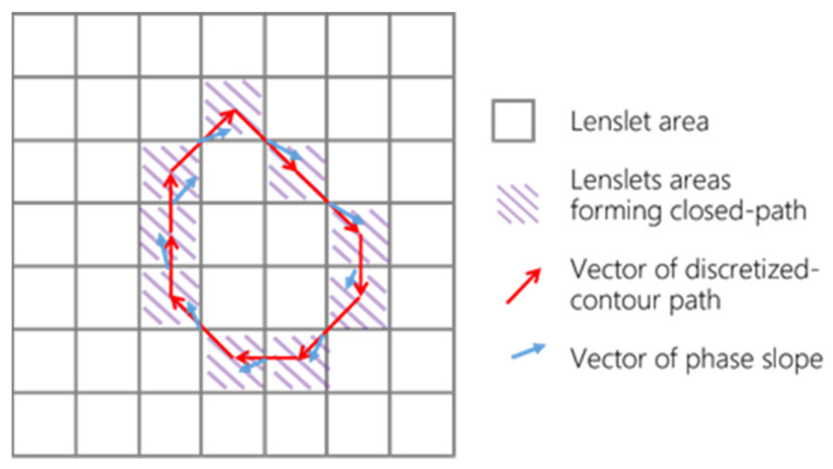
2. Generalized Contour-Sum Method

The contour-sum method was firstly proposed by Fried and Vaughn in 1992 [12] to prove that there is a branch cut (phase singularity) in the phase function of a light field with strong intensity variation. Since then, it has been adopted to detect OV beams using the phase slopes measured by an SH-WFS [20]. The essence of this method is that the circulation value of the phase gradient along a closed path enclosing the singularity point has a relationship with the TC value n, which is an integer and can be expressed as [20]:
n = 1 2 π C ϕ · d r ,
where C is a closed path, ϕ is the phase gradient, and d r is an infinitesimal displacement along the closed path C.
In practice, in order to determine the TC, we must discretize the line integral according to the geometrical configuration of sampling points, and accordingly rewrite Equation (1) as:
C i r = A 2 π k = 1 K S k · l k ,
where K is the number of sampling points along the closed path, and Sk and lk are the phase slope and discretized contour path of the k-th sampling point, respectively. In Equation (2), a constant A is introduced to compensate for the error caused by the discretization [24], and Cir is the TC value to be measured.
Specially, with the use of an SH-WFS, the discretization is realized by the lenslet array, and the phase slopes are simply obtained by the displacements of the focusing spots produced by the corresponding lenslets. Thus, the discretized contour paths connect the centers of the lenslet areas, forming the closed path. Figure 1 illustrates the generalized contour-sum method. In Figure 1, the square indicates the lenslet area, and the area marked with downward diagonal lines is the element forming the closed path. The discretized-contour path lk is represented by the red vector that connects the centers of the two adjacent elements in the closed path, and the blue vector Sk is the phase slope, which is the average of the phase slopes at the two adjacent elements.
The raw data from the SH-WFS measurement consist of a Hartmanngram of multiple focused spots. The five main steps of the GCSM are (1) preprocessing the Hartmanngram, including thresholding and segmentation; (2) calculating the phase slope of the individual lenslet area locations according to the SH-WFS working principle; (3) summing the intensity values of all pixels in each lenslet area to obtain the intensity sum value; (4) extracting a closed path from the intensity sum map; and (5) calculating the circulation, which is TC value of the OV beam.
In this algorithm, the closed path should be extracted from the intensity sum map, instead of from the Hartmanngram itself. This is because the intensity distribution behind the individual lenslet areas reflects the average distortion, but not the intensity distribution of the sub-wavefront incident into the lenslets. Since closed path determination is a crucial step, we focus on exploring the most proper closed path determination method in the rest of this paper.

3. Methods for Closed Path Determination

Basically, there are two strategies to determine a closed path from a given intensity sum map. One is to adaptively extract the closed path along the ridge of the intensity sum map. The reason why we search for the ridge elements is to ensure that all the measured phase slope data along the closed path are valid. Another strategy is to generate a closed path with a perfectly round shape, whose diameter and center could be adaptively varied within a given range. Hence, in this section, we explain closed path determination methods, following each strategy in detail. We introduce three methods that conform to the ridge-extracting strategy, which are watershed transformation (WT), MAIC extraction, and the combination of watershed transformation and MAIC extraction (WT-MAIC), as well as two methods that conform to the perfectly round circle generation strategy, which are the fixed-center perfectly round circle method (FC-PRCM) and the shifting-center perfectly round circle method (SC-PRCM).

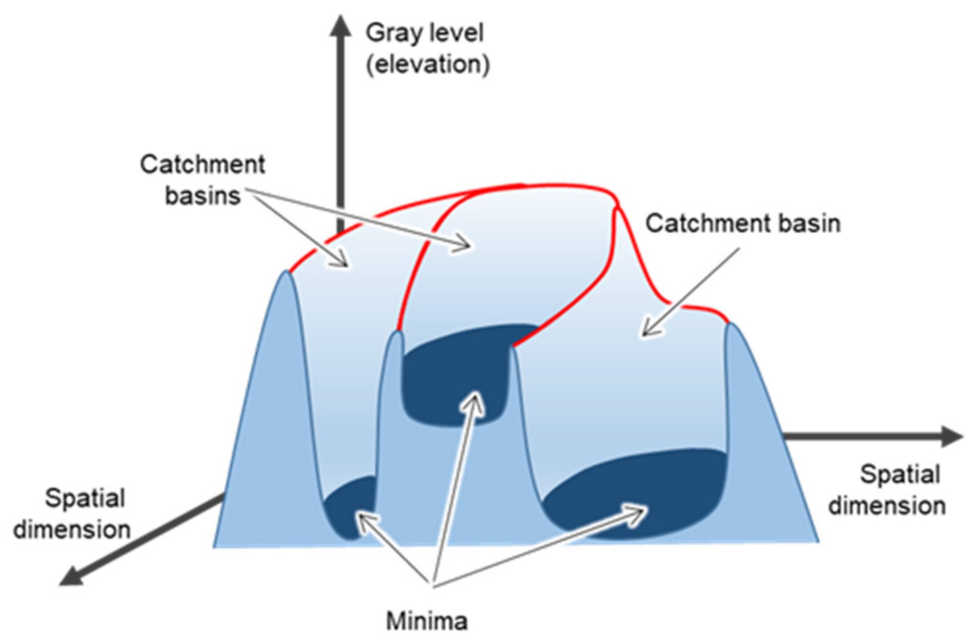
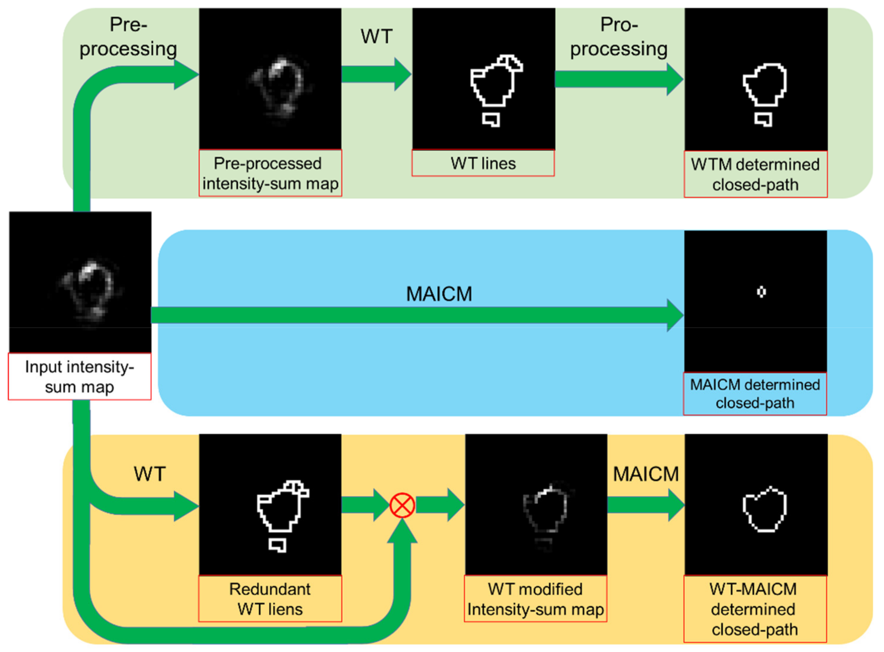
3.1. Watershed Transformation Method

Watershed transformation (WT) is a technique to extract ridges from an elevation map. This idea originated from the field of topography, and was firstly introduced as an image processing method by Beucher and Lantuéjoul [25]. Since then, many modifications and improvements to the method have been proposed [26,27,28,29]. The kernel of watershed transformation is to treat the two-dimensional grayscale input image as a topographic map, as shown in Figure 2, with the grayscale value of each individual point representing the elevation. After this transformation, the image is intuitively divided into several catchment basins, each of which corresponds to a regional minimum in the elevation dimension. The boundaries between diverse catchment basins are considered as the ridges, which are commonly termed watershed lines.
To perform watershed transformation on an image, flooding is the most commonly used strategy, and Meyer’s flooding algorithm is the corresponding extensively used algorithm [27]. Its core idea is to flood the entire topographic map, which is equivalent to raising the zero-elevation plane with time. With the flooding, the catchment basin corresponding to the global minimum is first filled with water, following which the other catchment basins start to fill with water one by one. After a certain amount of time, water from different catchment basins meet, and we build barriers to prohibit this phenomenon. The resulting barriers comprise the watershed lines, which correspondingly segment the input image into different regions.
Specifically, to apply watershed transformation on an intensity sum map to determine a closed path, we first perform preprocessing on the intensity sum map, such as thresholding and filtering [26], and then we perform the watershed transformation using the built-in function ‘watershed’ of MATLAB [30]. Moreover, considering that we aim to determine the net TC value in an OV beam, we should obtain only one closed path out of the multiple watershed lines. This can be realized by merging small regions into their neighboring large regions until there is only one region.

3.2. Maximum Average-Intensity Circle Extraction

The maximum average-intensity circle (MAIC) method has been proposed to extract a closed path from an intensity sum map for TC determination [24], as is briefly explained here. The basic process is to iteratively search the local peaks from the 2D intensity sum map and to connect these peak elements to form a closed path. The searching begins with the global maximum in the intensity sum map. The local maximum element from among several candidates of the eight neighbors of the current element is selected as the next element.

3.3. Watershed Transformed Maximum Average-Intensity Circle Extraction

Both WT and MAIC methods are simple and intuitive ways to obtain a closed path for circulation calculation, and they have equally excellent performance when the OV beam has little to no aberration. However, when the OV beam is severely distorted by aberration, the intensity sum map of the OV beam will have a shape far from a perfect circle, and may even split into several parts, resulting in both methods losing their efficiency. To further improve the performance under this severe aberration condition, we here propose a new method that combines WT and MAIC. In this method, we first perform watershed transformation on the intensity sum map, and then search for the ridge from among the elements on the watershed lines based on the MAIC algorithm. With the output of watershed transformation previously obtained, the influence of the element along the ridge and the noise can be significantly reduced, and thereby, a more proper closed path can be extracted. For simplicity, we named this method the watershed-transformed MAIC method (WT-MAICM).

3.4. Perfectly Round Circle Assignation

As mentioned above, besides the ridge-extracting strategy, adaptively generating an appropriate perfectly round circle according to the intensity sum profile of an OV beam is also a closed path determination strategy that is worthy of discussion. In general, the center position and radius are two integral parameters to generate a perfectly round circle. However, given an intensity sum profile, it is difficult to directly determine the most appropriate perfectly round circle. Consequently, in our previous research, we proposed to generate a group of concentric perfect circles, and chose the one for which the measured TC value had the maximum absolute value as the determined perfect round circle. The center position of the concentric perfect circles was determined as the nearest lenslet position from the centroid of the intensity sum map, while the lower and upper bounds of the radius variation range was determined by the radii of the inscribed and circumscribed circles of the intensity sum profile [24].
The performance of this generated perfectly round circle method (PRCM) as the closed path determination method to measure the TC value of a distorted OV beam is generally worse than that of the MAIC method [21,24]. The reasons are listed as follows:
  • The method determining the center position of the generated perfectly round circles by the centroid of intensity sum map is not optimal, because the nonuniformity along the azimuthal direction in the intensity sum distribution significantly affects the centroid calculation.
  • The center position as well as the radius are all forced to be integers.
  • The generated circles restricted to perfectly round shapes will unavoidably go through the low-intensity region, which means that invalid phase slope data will be obtained.
Notwithstanding, the generated circle should be fixed to a perfectly round shape to agree with the annular intensity sum profile and the position. Moreover, the radius should be forced to be an integer. This is because if we adaptively vary the shape or precisely calculate the position and radius and determine the phase slopes of the non-integer position by interpolation, the incurred complexity will go against our original goal of maintaining simplicity in the calculations. However, regarding the center position determination, the performance may be improved by shifting the center position within a proper region, referring to the radius variation. Although this dramatically increases the closed path determination time, we can accept a tradeoff between TC determination speed and accuracy if such a tradeoff manifests an improvement in the determination performance.
Consequently, in this paper, we propose a new, modified method for the generation of perfectly round circles based on the previously proposed method, where the modification is merely to shift the center position of the concentric perfectly round circles within an advisable region, as is further discussed in Section 5. For the sake of differentiation, we named this method the shifting-center perfectly round circle method (SC-PRCM) and the previously proposed perfectly round circle method the fixed-center perfectly round circle method (FC-PRCM).

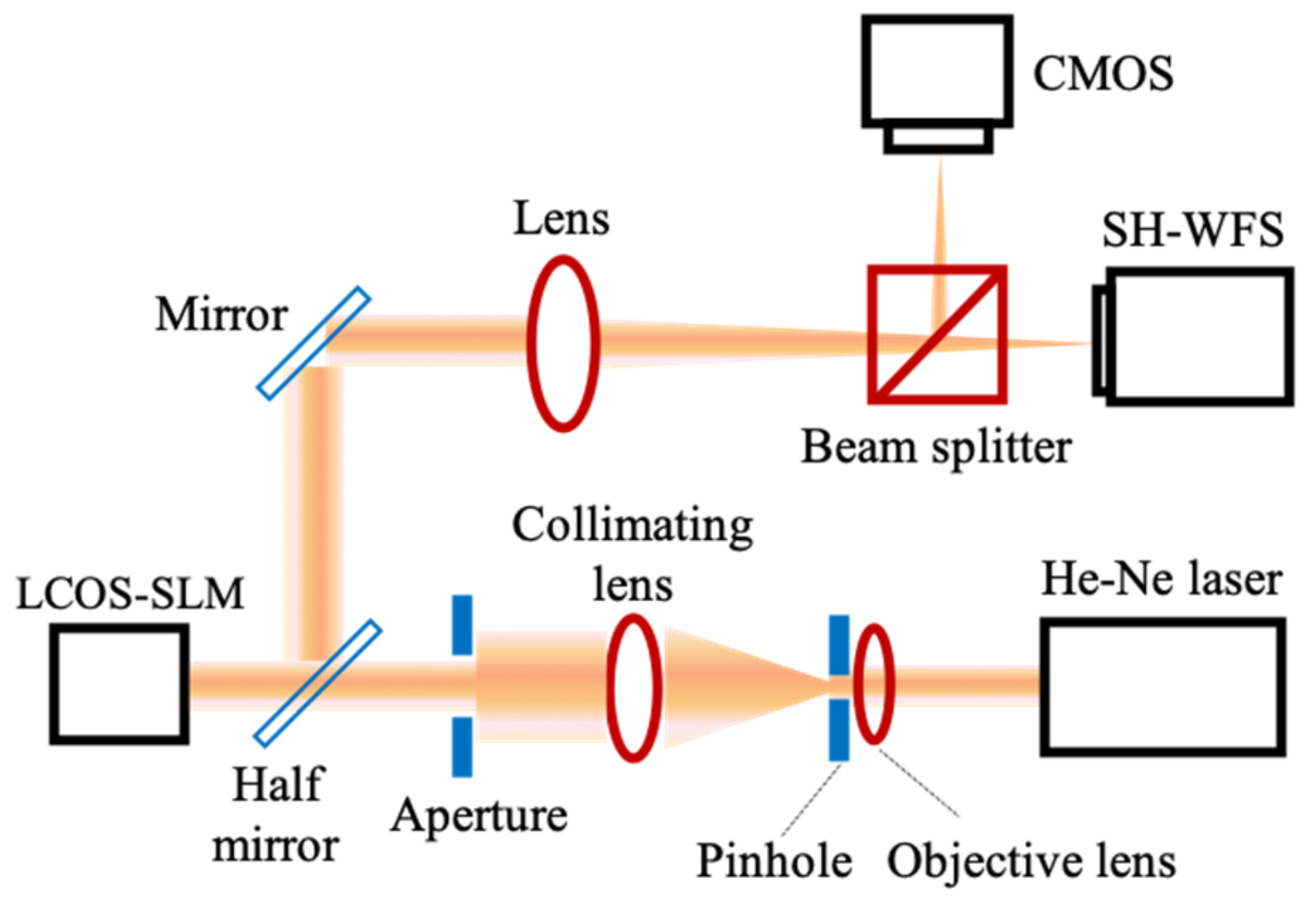
4. Experimental Setup

To verify the performance of these methods of closed path determination for the GCSM, we built an experimental setup, as shown in Figure 3 [24]. As shown in Figure 3, a collimated laser beam of wavelength 632.8 nm passed an aperture with a diameter of 4 mm, and was incident on a liquid crystal on silicon-spatial light modulator (LCOS-SLM). The LCOS-SLM was used to transform the incident beams into the optical vortex beams as well as bring aberrations into the beam. The beam reflected back from the LCOS-SLM was converged by a lens with a focal length of 2 m, and was split by a beam splitter into two beams. Finally, we used an SH-WFS to record the Hartmanngram and a complementary metal-oxide semiconductor (CMOS) camera to check and record the intensity profile of the OV beam. The LCOS-SLM was set at the front focal plane of the lens, while the SH-WFS as well as the CMOS camera were both located at the back focal plane of the lens.
The LCOS-SLM (Hamamatsu, X10468-01) was a pure phase modulator consisting of 792 × 600 pixels with a pixel size of 20 × 20 µm [31]. The SH-WFS consisted of two elements: a square grid lenslet array with a pitch size of 200 µm and focal length of 11 mm, and a high-speed intelligent vision sensor with 512 × 512 pixels and a pixel size of 20 × 20 µm [32]. The SH-WFS was mounted on a mechanical platform that could be moved along the horizontal direction. The movement was precisely controlled by a stepping motor system. The CMOS camera was 2592 × 2048 pixels and had a pixel size of 4.8 × 4.8 µm.

5. Results and Discussion

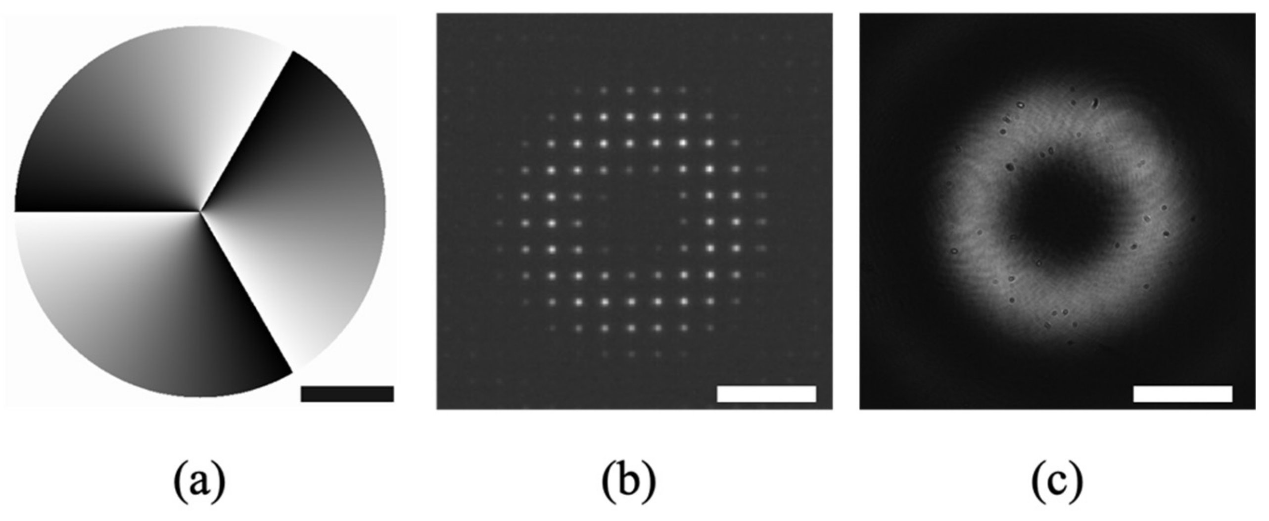
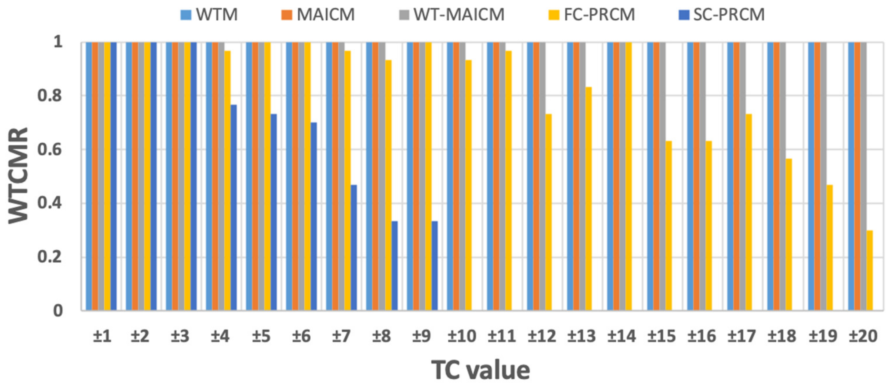
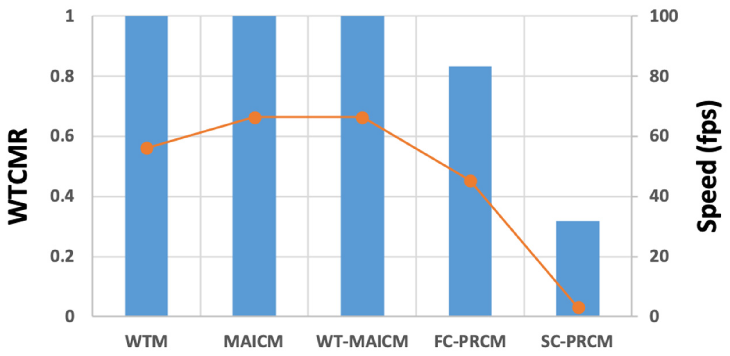
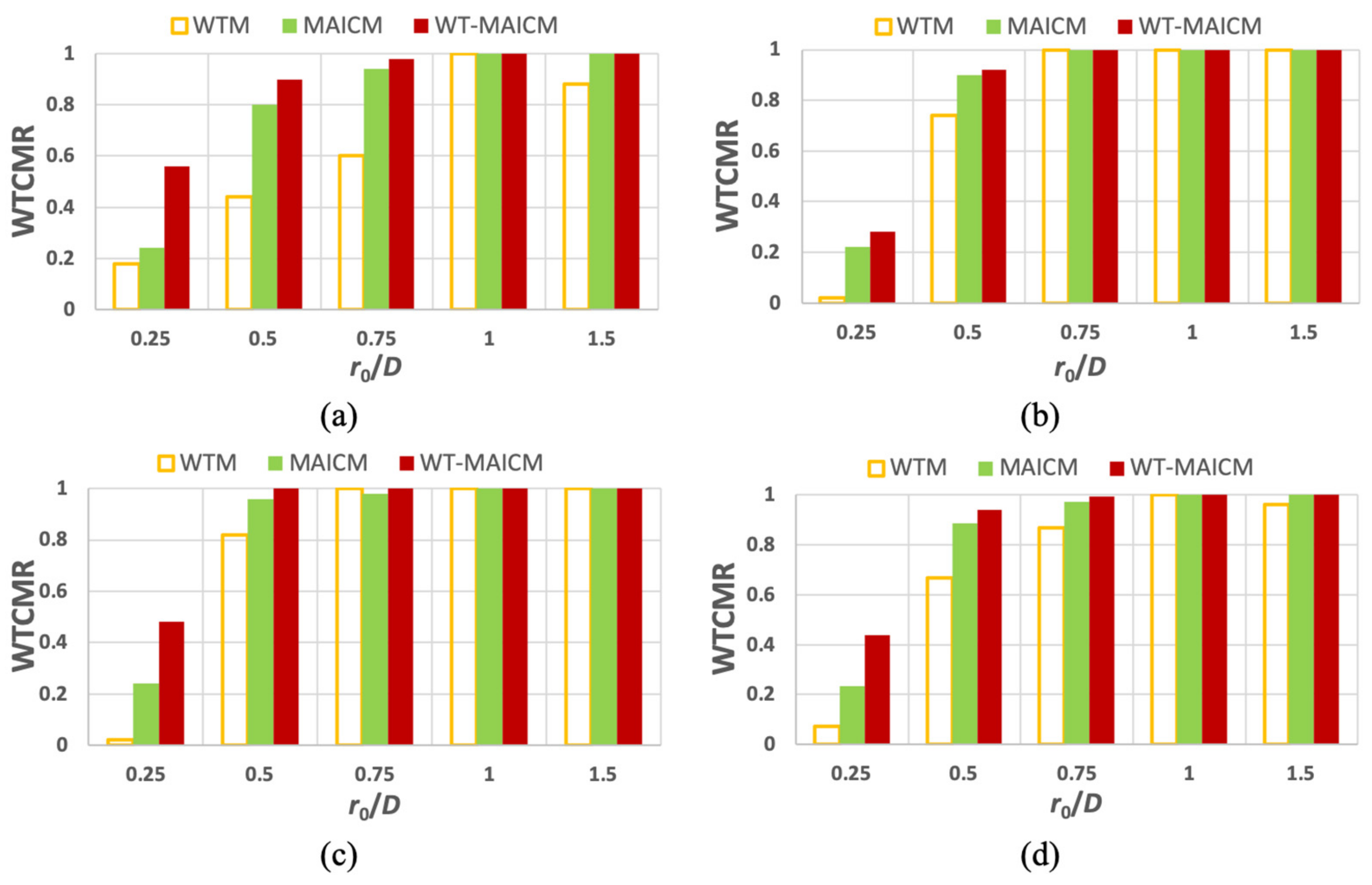
5.1. Performance Comparison Based on Aberration-Free OV Beams

To compare the above five closed path determination methods, we first evaluated the performance under the aberration-free OV beam condition. In the experiments, we displayed various computer-generated holograms (CGHs) with a spiral phase structure on the LCOS-SLM to generate an OV beam with TC values ranging from ± 1 to ± 20. In order to enrich the data amount as well as eliminate the randomness, for each TC value, we repeatedly recorded the Hartmanngrams at 15 different SH-WFS positions by laterally moving the mechanical platform. Hence, we obtained a total of 600 Hartmanngrams (40 TC values and 15 SH-WFS positions). Figure 4 shows an example of the spiral phase pattern displayed on LCOS-SLM, and the corresponding Hartmanngram as well as the intensity profile image respectively recorded by SH-WFS and CMOS camera.
As described in Section 2, for each recorded Hartmanngram, we first performed the necessary preprocessing, and then summed all the pixel values in each lenslet region to obtain the intensity sum map and measured the phase slopes at the lenslet positions according to the SH-WFS working principle. After that, we used each of the studied five methods to determine the closed path, and then utilized the generalized counter-sum method to calculate the TC value.
Considering that the theoretical TC value is an integer, for TC measurement, if the absolute difference between the measured TC value and the theoretical TC value is lower than 0.5, the measured TC value will be identical to the theoretical TC value after rounding—we define this as a well-determined TC measurement. Based on this definition, we introduced a parameter, the well-determined TC measurement ratio (WTCMR), which is the percentage of well-determined TC measurements within a given set of TC measurements, to quantitatively compare the performance of the diverse closed path determination methods.
The performance evaluation results of the individual closed path determination methods are given in Figure 5 and Figure 6. In Figure 5, each value is the WTCMR of a group of 30 measurements (15 positions for both positive and negative TC values), while in Figure 6, the WTCMR is the statistical average of all 600 measurements. Figure 6 also shows the corresponding processing speed of the individual methods in terms of frames per second, which was measured on an Intel Core i7 computer with a CPU frequency of 3.7 GHz and 16 GB of RAM.
As shown in Figure 5 and Figure 6, the WT, MAIC, and WT-MAIC methods performed perfectly, since the WTCMR was shown to be 100% for all tested TC values. However, the WTCMR of the FC-PRCM and the SC-PRCM was not always 100%, even when measuring aberration-free OV beams. Moreover, the performance of these methods deteriorated with the increase of the TC value. The SC-PRCM was the worst method in terms of both the WTCMR and the computing speed.
Considering that the TC determination progress is the same apart from the closed path being determined by diverse closed path determination methods, the reason for the differences in performance was exclusively due to the differences in the determined closed paths. To concretely demonstrate these differences, as well as the origin of the differences and why this factor significantly changes the TC determination performance, we present some examples in Figure 7. In this figure, the columns from left to right indicate the results using the WTM, MAICM, WT-MAICM, FC-PRCM, and SC-PRCM, and the rows from top to bottom are the inputted OV beams of TC values of 10 (top row), 15 (middle row), and 20 (bottom row). In Figure 7, each row has the same intensity sum map, and the red circle superimposed on the intensity sum map is the closed path extracted by the individual method.
From the figure, it can be seen that the WTM, MAICM, and WT-MAICM can properly extract closed paths passing through the ridge elements, thus obtaining precise TC values. On the other hand, for the FC-PRCM and SC-PRCM, the closed path might go through the low-intensity sum regions where the measured phase slopes are invalid. When the TC value of the OV beam varied from 10 to 15 to 20, the effects of the nonuniformity of the intensity sum map along the azimuthal direction increased. As a result, the closed path deviated more from the ridge elements and went through the low-intensity regions, generating a large error in the measured TC values. As for the SC-PRCM, its performance deteriorated more compared with that of the FC-PRCM. This reveals that simply shifting the center position of the concentric perfectly round circles does not improve, but rather reduces the performance. We believe that this is because shifting the center position of perfectly round circles may deviate the centers even further from the real position of the vortex, and thus they become liable to be affected by the invalid slope data in the low-intensity regions. Considering that we chose the generated perfectly round circle with the maximum absolute calculated TC value as the determined closed path, the SC-PRCM mostly output a measured TC value larger than the theoretical value. Moreover, in combination with the poor performance of the FC-PRCM, we found that the unified closed path determination criterion in the PRCM strategy, which is to select the generated perfectly round circle with the maximum absolute calculated TC value as the determined closed path, is not entirely rational, although it is simple.
The above finding was also supported by analyzing the errors of the measured TC values. Figure 8 shows the histogram distributions of the absolute error (AE) of TC measurements, wherein the x-axis is the interval of the AE, which is the absolute difference between the measured TC value and the theoretical TC value, and the y-axis is the frequency of the 600 measurements. From the distribution, we can view the striking difference between the performances of the WTM, MAICM, and WT-MAICM, and those of the FC-PRCM and SC-PRCM. Almost all of the AEs of the former three methods are concentrated within the value interval of 0 to 0.2; on the contrary, the AEs are distributed in a partly uniform pattern with one-sixth within the value interval of over 0.5 when using the FC-PRCM, while the majority are in the value interval of over 0.5 when using the SC-PRCM. This phenomenon profoundly influences the correct rate of TC determination when we shrink the confidence interval of the well-determined TC measurements. For example, when using AE < 0.3 as a criterion for the well-determined TC measurement definition, the WTCMR values of the WTM, MACIM, and WT-MAICM are still over 99%; however, those of the FC-PRCM and SC-PRCM drop to 63.3% and 19.7%, respectively.
According to the previous discussions, we concluded that the FC-PRCM and SC-PRCM are not appropriate as closed path determination methods, and that generating a perfectly round circle is not a plausible nor practical closed path determination strategy. Therefore, we started to just involve the other three closed path determination methods in the following comparison.

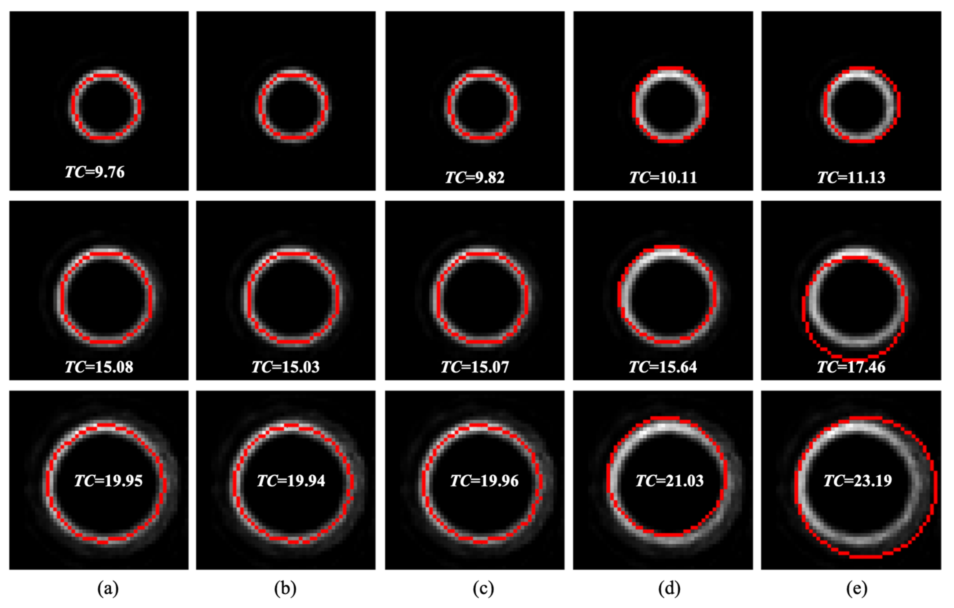
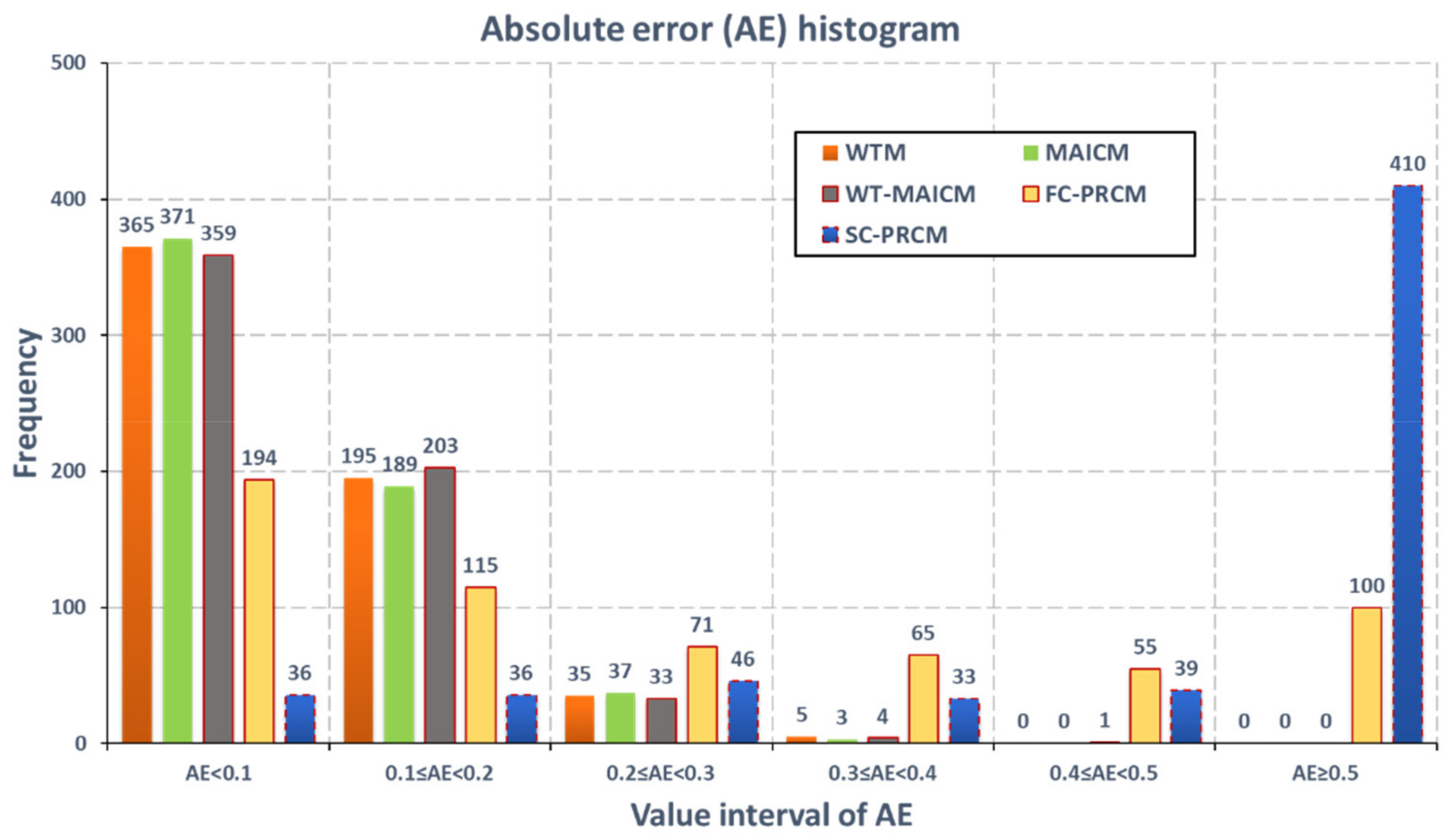
5.2. Performance Comparison Based on Distorted OV Beams

Many practical applications of OV beams, e.g., free-space optical communication and optical remote metrology, require the determination of the TC value of the OV beam after its propagation over a certain distance in the atmosphere. Consequently, it is vital to evaluate and compare these methods for OV beams distorted by atmospheric turbulence. Generally, a turbulent atmosphere can be treated as an inhomogeneous refractive index media, featured by the structure parameter C n 2 [33], and its impact on the light beam propagating through it can be accumulated as phase screens [34]. Supposing the turbulence satisfies the Kolmogorov model, the phase screen can be simulated through the Zernike polynomial [35]. The coefficients of the Zernike polynomial are related to the normalized correlation length r0/D, where r0 is the Fried parameter and D is the beam size [36].
In the experiments, considering that the beam size used in our optical system was 4 mm, we chose r0 to be 1, 2, 3, 4, and 6 mm, and the normalized correlation length r0/D was chosen to be 0.25, 0.5, 0.75, 1, and 1.5. Under each r0/D value, we performed 50 random realizations of phase screens, which were then separately superposed with the spiral phase pattern (SPPs) whose TC values were 1, 5, and 10. Therefore, we generated 750 phase patterns altogether (three TC values, five r0/D values, and 50 phase screens). Afterwards, we displayed the phase patterns one by one on the LCOS-SLM and recorded the corresponding Hartmanngrams. The SH-WFS did not move herein, because we had already generated 50 diverse phase patterns under each condition for repeated testing. For each Hartmanngram, we respectively used WTM, MAICM, and WT-MAICM as the closed path determination method, and determined the TC value by the generalized contour-sum method.
The experimental results evaluated by the WTCMR are given in Figure 9, where Figure 9a–c corresponds to a set of 50 measurements for the individual TC, and Figure 9d is the mean of these measurements.
Based on the experimental results, we found that the general tendency of TC measurement accuracy increased along with the increase of r0/D, which means the atmospheric turbulence becomes gentler. Moreover, when changing the closed path determination method from WTM to MAICM to WT-MAICM, the TC determination accuracy improved, especially when the atmospheric turbulence was severe. Supposing the accredited WTCMR to be over 0.9, we found that the limitations of r0/D for WTM, MAICM, and WT-MAICM were around approximately 0.75–1, 0.5–0.75, and 0.25–0.5, respectively.
Figure 10 is an example specifically illustrating why the WT-MAICM has a better performance than the WTM and MAICM. Here, the OV beam to be measured has a TC value of 10 and a turbulence strength parameter r0/D of 0.25. The top, middle, and bottom rows show the closed path determination processes and corresponding results when utilizing WTM, MAICM, and WT-MAICM separately. From the significantly different determined closed paths, we can see that when the turbulence is severe, the distorted OV beam can have extremely nonuniform regions. These nonuniform regions can trap the MAICM searching process into a local loop (middle row), or lead the WTM-determined closed path to be more than one part (top row), which conflicts with the aim of extracting only one closed path; these results eventually deteriorate the performance of the WTM and MAICM.

6. Conclusions

In this paper, we presented an experimental comparison of five closed path determination methods for the use of GCSM to detect the TC of an OV beam. These five methods are the previously proposed MAICM and FC-PRCM, and three newly proposed methods: the WTM, WT-MAICM, and SC-PRCM. These methods come from two strategies: WTM, MAICM, and WT-MAICM belong to the strategy of ridge extraction, and FC-PRCM and SC-PRCM are derived from the strategy of PRC assignation. The codes for the algorithms are available from the authors by email. The methods were tested with an optical setup that used a LCOS-SLM as an OV beam, and an aberration generator and an SH-WFS located at the far-field plane to measure the OV beams. Two types of evaluation experiments were performed. One was under the condition that the OV beam had hardly any aberration, and the other was under the condition that the OV beam was distorted by simulated atmospheric turbulence. The experimental results indicate that the methods with ridge extraction outperform those based on PRC assignation in terms of both the well-determined detection rate and the processing speed.
Under the condition of an aberration-free OV beam, the WTM, MAICM, and WT-MAICM performed excellently and achieved WTCMR values of 100%. On the other hand, the WTCMR values of the FC-PRCM and SC-PRCM were not always 100% and the performance was reduced with the increase of the TC value. What is more, the SC-PRCM was found to be the worst method in terms of both the WTCMR and the processing speed. There are a number of reasons that can explain the poor performance of the PRC assignation strategy, but the major factors are that the generated circle is prone to deviate from the OV center and go through regions with low intensity as well as invalid phase slope data, which are caused by nonuniformity in the intensity sum map along the azimuthal direction. The performance of the SC-PRCM was worse than that of the FC-PRCM, indicating that simply shifting the center of the PRC is not a suitable solution, and the maximum absolute TC value hunting criterion in the PRC assignation strategy lacks rationality.
In the case of measuring distorted OV beams, the WTM, MAICM, and WT-MAICM show certain differences in term of the WTCMR, especially when the turbulent strength is high. Among these three methods, the WT-MAICM shows the strongest robustness against distortion, and the WTM was found to be the weakest. The limits of r0/D to achieve WTCMR > 90% were around 0.75–1, 0.5–0.75, and 0.25–0.5 for the WTM, MAICM, and WT-MAICM, respectively, in terms of normalized correlation length. Overall, these results reveal that adaptively determining the closed path is necessary for GCSM in detecting the TC from a distorted OV beam.

Author Contributions

Conceptualization, D.W. and H.H.; funding acquisition, H.L.; methodology, D.W. and H.H.; project administration, H.H.; resources, H.T.; supervision, H.L. and H.T.; validation, D.W. and H.H.; writing—original draft, D.W.; writing—review and editing, D.W. and H.H.

Funding

Shenzhen Innovation Funding (No: JCYJ20170818164343304, JCYJ20170816172431715); National Natural Science Foundation of China (No: U1809204, 61525106, 61427807, 61701436); National Key Technology Research and Development Program of China (No: 2017YFE0104000, 2016YFC1300302).

Acknowledgments

We gratefully acknowledge A. Hiruma and T. Hara for their support and encouragement throughout this study. Wang thanks the exchange program between Hamamatsu Photonics K.K. and Zhejiang University. The support from the above funding organizations is also gratefully acknowledged.

Conflicts of Interest

The authors declare no conflict of interest.

References

  1. Bozinovic, N.; Yue, Y.; Ren, Y.; Tur, M.; Kristensen, P.; Huang, H.; Willner, A.E.; Ramachandran, S. Terabit-scale orbital angular momentum mode division multiplexing in fibers. Science 2013, 340, 1545–1548. [Google Scholar] [CrossRef] [PubMed]
  2. Zhang, D.; Feng, X.; Huang, Y. Encoding and decoding of orbital angular momentum for wireless optical interconnects on chip. Opt. Express 2012, 20, 26986–26995. [Google Scholar] [CrossRef] [PubMed]
  3. Wang, J.; Yang, J.Y.; Fazal, I.M.; Ahmed, N.; Yan, Y.; Huang, H.; Ren, Y.; Yue, Y.; Dolinar, S.; Tur, M.; et al. Terabit free-space data transmission employing orbital angular momentum multiplexing. Nat. Photonics 2012, 6, 488. [Google Scholar] [CrossRef]
  4. Li, S.; Wang, J. Experimental demonstration of optical interconnects exploiting orbital angular momentum array. Opt. Express 2017, 25, 21537–21547. [Google Scholar] [CrossRef] [PubMed]
  5. Chu, S. Laser Manipulation of Atoms and Particles. Science 1991, 253, 861–866. [Google Scholar] [CrossRef] [PubMed]
  6. Otsu, T.; Ando, T.; Takiguchi, Y.; Ohtake, Y.; Toyoda, H.; Itoh, H. Direct evidence for three-dimensional off-axis trapping with single Laguerre-Gaussian beam. Sci. Rep. 2014, 4, 4579. [Google Scholar] [CrossRef] [PubMed] [Green Version]
  7. Liphardt, J.; Dumont, S.; Smith, S.B.; Tinoco, I.; Bustamante, C. Equilibrium information from nonequilibrium measurements in an experimental test of Jarzynski’s equality. Science 2002, 296, 1832–1835. [Google Scholar] [CrossRef] [PubMed]
  8. Sato, S.; Fujimoto, I.; Kurihara, T.; Ando, S. Remote six-axis deformation sensing with optical vortex beam. In Proceedings of the Free-Space Laser Communication Technologies XX, San Jose, CA, USA, 19–24 January 2008. [Google Scholar]
  9. Wang, W.; Yokozeki, T.; Ishijima, R.; Takeda, M.; Hanson, S.G. Optical vortex metrology based on the core structures of phase singularities in Laguerre-Gauss transform of a speckle pattern. Opt. Express 2006, 14, 10195–10206. [Google Scholar] [CrossRef] [PubMed]
  10. Fujimoto, I.; Sato, S.; Kim, M.Y.; Ando, S. Optical vortex beams for optical displacement measurements in a surveying field. Meas. Sci. Technol. 2011, 22, 105301. [Google Scholar] [CrossRef]
  11. Nye, J.F.; Berry, M.V. Dislocations in wave trains. Proc. R. Soc. Lond. A Math. Phys. Sci. 1974, 336, 165–190. [Google Scholar] [CrossRef]
  12. Fried, D.L.; Vaughn, J.L. Branch cuts in the phase function. Appl. Opt. 1992, 31, 2865–2882. [Google Scholar] [CrossRef] [PubMed]
  13. Rockstuhl, C.; Ivanovskyy, A.A.; Soskin, M.S.; Salt, M.G.; Herzig, H.P.; Dändliker, R. High-resolution measurement of phase singularities produced by compute-generated holograms. Opt. Commun. 2004, 242, 163–169. [Google Scholar] [CrossRef]
  14. Chen, R.; Zhang, X.; Zhou, Y.; Ming, H.; Wang, A.; Zhan, Q. Detecting the topological charge of optical vortex beams using a sectorial screen. Appl. Opt. 2017, 56, 4868–4872. [Google Scholar] [CrossRef] [PubMed]
  15. Hickmann, J.M.; Fonseca, E.J.; Soares, W.C.; Chávez-Cerda, S. Unveiling a truncated optical lattice associated with a triangular aperture using light’s orbital angular momentum. Phys. Rev. Lett. 2010, 105, 053904. [Google Scholar] [CrossRef] [PubMed]
  16. Prabhakar, S.; Kumar, A.; Banerji, J.; Singh, R.P. Revealing the order of a vortex through its intensity record. Opt. Lett. 2011, 36, 4398–4400. [Google Scholar] [CrossRef]
  17. Schulze, C.; Naidoo, D.; Flamm, D.; Schmidt, O.A.; Forbes, A.; Duparré, M. Wavefront reconstruction by modal decomposition. Opt. Express 2012, 20, 19714–19725. [Google Scholar] [CrossRef] [Green Version]
  18. Li, S.; Wang, J. Simultaneous demultiplexing and steering of multiple orbital angular momentum modes. Sci. Rep. 2015, 5, 15406. [Google Scholar] [CrossRef] [Green Version]
  19. Platt, B.C.; Shack, R. History and principles of Shack-Hartmann wavefront sensing. J. Refract. Surg. 2001, 17, S573–S577. [Google Scholar] [CrossRef]
  20. Chen, M.; Roux, F.S.; Olivier, J.C. Detection of phase singularities with a Shack-Hartmann wavefront sensor. J. Opt. Soc. Am. A 2007, 24, 1994–2002. [Google Scholar] [CrossRef] [Green Version]
  21. Le Bigot, E.O.; Wild, W.J. Theory of branch-point detection and its implementation. J. Opt. Soc. Am. A 1999, 16, 1724–1729. [Google Scholar] [CrossRef]
  22. Huang, H.; Luo, J.; Matsui, Y.; Toyoda, H.; Inoue, T. Eight-connected contour method for accurate position detection of optical vortices using Shack–Hartmann wavefront sensor. Opt. Eng. 2015, 54, 111302. [Google Scholar] [CrossRef]
  23. Luo, J.; Huang, H.; Matsui, Y.; Toyoda, H.; Inoue, T.; Bai, J. High-order optical vortex position detection using a Shack-Hartmann wavefront sensor. Opt. Express 2015, 23, 8706–8719. [Google Scholar] [CrossRef] [PubMed]
  24. Wang, D.; Huang, H.; Matsui, Y.; Tanaka, H.; Toyoda, H.; Inoue, T.; Liu, H. Aberration-resistible topological charge determination of annular-shaped optical vortex beams using Shack–Hartmann wavefront sensor. Opt. Express 2019, 27, 7803–7821. [Google Scholar] [CrossRef] [PubMed]
  25. Beucher, S.; Lantuejoul, C. Use of watersheds in contour detection. In Proceedings of the International Workshop Image Processing, Real-Time Edge and Motion Detection/ Estimation, CCETT/IRISA, Rennes, France, 17–21 September 1979. [Google Scholar]
  26. Meyer, F.; Beucher, S. Morphological segmentation. JVCIP 1990, 1, 21–46. [Google Scholar] [CrossRef]
  27. Meyer, F. Topographic distance and watershed lines. Signal. Process. 1994, 38, 113–125. [Google Scholar] [CrossRef]
  28. Vincent, L.; Soille, P. Watersheds in digital spaces: An efficient algorithm based on immersion simulations. IEEE Trans. Pattern Anal. Mach. Intell. 1991, 13, 583–598. [Google Scholar] [CrossRef]
  29. Osma-Ruiz, V.; Godino-Llorente, J.I.; Sa´enz-Lecho´n, N.; Go´mez-Vilda, P. An improved watershed algorithm based on efficient computation of shortest paths. Pattern Recognit. 2007, 40, 1078–1090. [Google Scholar] [CrossRef]
  30. Watershed Function in MathWorks. Available online: https://www.mathworks.com/help/images/ref/watershed.html?s_tid=srchtitle (accessed on 11 August 2019).
  31. Inoue, T.; Tanaka, H.; Fukuchi, N.; Takumi, M.; Matsumoto, N.; Hara, T.; Yoshida, N.; Igasaki, Y.; Kobayashi, Y. LCOS spatial light modulator controlled by 12-bit signals for optical phase-only modulator. Proc. SPIE 2007, 6487, 64870Y. [Google Scholar]
  32. Sugiyama, Y.; Takumi, M.; Toyoda, H.; Mukozaka, N.; Ihori, A.; Kurashina, T.; Nakamura, Y.; Tonbe, T.; Mizuno, S. A high-speed CMOS image sensor with profile data acquiring function. IEEE J. Solid State Circuits 2005, 40, 2816–2823. [Google Scholar] [CrossRef]
  33. Tyson, R.K. Principles of Adaptive Optics; Academic: Salt Lake City, UT, USA, 1991. [Google Scholar]
  34. Kolmogorov, A.N. A refinement of previous hypotheses concerning the local structure of turbulence in a viscous incompressible fluid at high Reynolds number. J. Fluid Mech. 1962, 13, 82–85. [Google Scholar] [CrossRef] [Green Version]
  35. Roddier, N.A. Atmospheric wavefront simulation using Zernike polynomials. Opt. Eng. 1990, 29, 1174–1180. [Google Scholar] [CrossRef]
  36. Fried, D.L. Statistics of a geometric representation of a wavefront distortion. J. Opt. Soc. Am. 1965, 55, 1427–1435. [Google Scholar] [CrossRef]
Figure 1. Graph illustrating the generalized contour-sum method.
Applsci 09 03956 g001
Figure 2. A diagram to illustrate the topographic map of an image after performing watershed transformation. The red curves are the watershed lines.
Applsci 09 03956 g002
Figure 3. Schematic diagram of the experimental setup.
Applsci 09 03956 g003
Figure 4. Example of (a) spiral phase pattern, (b) Hartmanngram, and (c) intensity profile recorded by the complementary metal-oxide semiconductor (CMOS) camera. The bar indicates 1 mm.
Applsci 09 03956 g004
Figure 5. Well-determined topological charge (TC) measurement ratio (WTCMR) distributions of the five closed path determination methods when the TC value changes from ±1 to ± 20.
Applsci 09 03956 g005
Figure 6. TC determination performances of five closed path determination methods in terms of the WTCRM (bars) and speed in frames per second (fps) (points). Each bar or point is the statistical average of all 600 measurements under the corresponding closed path determination method.
Applsci 09 03956 g006
Figure 7. Examples showing the differences of the closed paths (the red circles) and the TC values determined by (a) the watershed transformation method (WTM), (b) the maximum average-intensity circle method (MAICM), (c) the WT-MAICM, (d) the fixed-center perfectly round circle method (FC-PRCM), and (e) the shifting-center (SC-PRCM). The theoretical TC values are 10 (top row), 15 (middle row), and 20 (bottom row). In each image, the background is the intensity sum map, and the red circle is the closed path determined by the individual methods. The corresponding measured TC value is labeled in each image.
Applsci 09 03956 g007
Figure 8. Absolute error (AE) histograms of 600 TC measurements separately using WTM, MAICM, WT-MAICM, FC-PRCM, and SC-PRCM. The number over each bar indicates the number of the measurements whose AE values are within the corresponding interval.
Applsci 09 03956 g008
Figure 9. TC determination performance of three methods under different atmospheric turbulence conditions, where (a) is under TC = 1, (b) is under TC = 5, (c) is under TC = 10, and (d) is the average of (a), (b), and (c).
Applsci 09 03956 g009
Figure 10. Closed path determination processes and results using the WTM (top row), MAICM (middle row), and WT-MAICM (bottom row).
Applsci 09 03956 g010

