Abstract
With the growth in demand for energy and the boom in energy internet (EI) technologies, comes the multi-energy complementary system. In this paper, we first model the components of the micro-energy-grid for a greenhouse, and then analyzed two types of protected agriculture load: time-shifting load and non-time-shifting load. Next, multi-scenario technology is directed against the uncertainty of photovoltaic (PV). Latin Hypercube Sampling (LHS) and the backward reduction algorithm are the two main methods we use to generate the representative scenarios and their probabilities, which are the basis for PV prediction in day-ahead scheduling. Third, besides the time of day (TOD) tariff, we present a model using real-time pricing of consumers’ electricity load, which is proposed to compare consumers’ demand response (DR). Finally, we establish a new optimization model of micro-energy-grid for greenhouses. By calculating the dispatch of electricity, heat, energy storage and time-shifting load under different conditions, the local consumption of PV and the comprehensive operational cost of micro-energy-grid can be analyzed. The results show that a storage device, time-shifting load and real-time pricing can bring more possibilities to the micro-energy-grid. By optimizing the time schedule of time-shifting load, the cost of the greenhouse is reduced.
1. Introduction
Energy is the basis of human survival and development, as well as the key element of industrial production and residents’ life. How to reduce environmental pollution in the process of using energy while ensuring the sustainable supply of energy is the common concern of today’s society [,,]. Conventional energy systems are mutually independent and different energy sources cannot cooperate to produce a comprehensive optimal scheme [], thus energy efficiency is reduced. An integrated energy system (IES) combines independent energy systems together. As an important carrier of energy internet (EI), IES monitors and manages the production, transmission, storage and utilization of various energy sources at the system level. IES can realize not only multi-energy complementary, but also stepped utilization of energy. It meets the abundant demands of users for diverse energy forms, such as electricity, heating, cooling and gas, as well as improves the utilization efficiency of renewable energy.
At present, research on IES mainly focuses on a series of problems about simulation modeling and optimization scheduling. Geidl et al. [] first conceived the basic architecture of the energy hub (EH). As an energy management center, EH is widely used in IES modeling. Based on the fundamental concepts and modeling methods of EH, Wang et al. [] summarized the optimization and operation of EH planning. Gan et al. [] established a multi-energy flow scheduling model including combined cooling, heating and power (CCHP) as well as distributed wind power and PV. In addition, they analyzed its impact on renewable energy consumption and overall cost. In [], a general method for CCHP optimal scheduling is proposed, Moreover, a multi-energy coordinated optimal scheduling model including CCHP, wind power and photovoltaic output, ice storage air conditioning and battery energy storage is established. The authors used the scenario reduction method to deal with the wind power and PV uncertainty problem.
DR is able to timely feedback power supply and demand, which has great significance to improve the operating efficiency of the power system and maintain its stable operation []. Nowadays, the demand response of the electricity market is mainly divided into two types: price-based DR and incentive-based DR. Cui et al. [] established a scheduling model, which was based on solar-thermal power station and price-based DR, to improve the capacity of wind power absorption through coordinated scheduling on both sides of source and load. In [], the authors established a scheduling model for incentive-based DR, and performed reliability assessment and economic analysis on the test system based on Monte Carlo simulation method. DR can be adjusted by controlling load demand, which can make consumers’ electricity habits more reasonable. This process can maximize the system efficiency by reducing unnecessary spinning reserve, installed capacity and peak–trough load difference, also optimizing load curve through peak-cut and trough-fill. Compared with the traditional one, the interconnections among different energy systems in IES improve the agility of consumers’ response. For example, in the process of cogeneration, combined heating and power (CHP) on the user’s side, the demand can be satisfied by adjusting power or heat output separately [,,]. It is meaningful and potential in the future to reconcile the DR and IES.
Northwest China has sufficient solar and wind energy [,], thus during 2013–2017, the PV cumulative installed capacity kept increasing and exceeded 30,000 MW. To achieve the goal of poverty alleviation in rural areas by 2020, China implements the strategy of supporting the poor in rural areas of western China. Since renewable energy is uncertain, robust optimal scheduling algorithms [,] are usually applied to cope with this issue. To accommodate more renewable energy sources, flexibility from the power load is frequently adopted [,].
Now, the installed capacity of PV in northwest China is increasing rapidly. However, due to the restriction of distribution grid, PV power generation does not have the ability to feed back the distribution network, but only be absorbed locally. This is a great waste of PV resources. On the other hand, intelligent agriculture and protected agriculture, as new modes of electricity use in agriculture, are more diversified and gradually promoted in rural areas. The coordinated application of multi-energy in IES has created favorable conditions for local PV absorption. Meanwhile, the protected agriculture load is usually time-shifting and schedulable, which is an excellent consumer-side response resource. Therefore, reasonable dispatching and planning of time-shifting load in agricultural production is also a measure of DR with rural characteristics.
2. Model
2.1. Micro-Energy-Grid Model
In the greenhouse micro-energy-grid, electricity comes from CHP by burning biogas and PV power generation devices set up on the roof of the greenhouse. Besides, it is connected with the power distribution network: when the power is insufficient, it can purchase electricity directly from the upper level. Thermal energy in the greenhouse micro-energy-grid also comes from CHP by burning methane and air source heat pumps (ASHPs). Thus, the electricity and heat in the micro-energy-grid are coupled. Batteries and phase change thermal storage (PCTS) as energy storage components can store surplus electricity and heat, and affect time-shifting. The greenhouse also has biogas digester, which uses heat pump in the digester to consume electricity and promote microbial fermentation producing biogas. The basic on-line diagram of the greenhouse micro grid is shown in Figure 1.
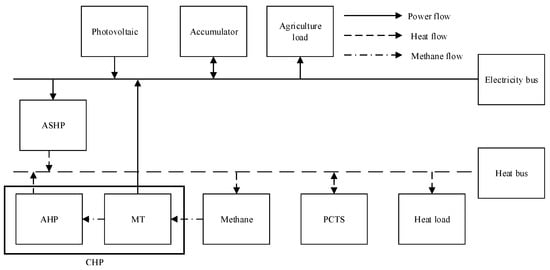
Figure 1.
The basic on-line diagram of greenhouse micro grid.
CHP, ASHPs and transformer are the main components of the agricultural greenhouse micro-energy-grid. CHP includes microturbine, biogas digester and absorption heat pump (AHP). All parts work together to realize conversion and the process can be seen in Table 1. Micro-energy-grid’s energy is supplied from biogas, PV and upper level power grid. Under the condition that energy hub (EH) meets the electricity and heat demands of the greenhouse, the surplus PV power generation can be processed on the grid.

Table 1.
Energy conversion of components in energy hub.
2.2. CHP Model
In the greenhouse, biogas not only can be used as primary energy for electricity and heat supply, but also can produce carbon dioxide by burning. Carbon dioxide can fertilize plants, which is an effective utilization of the biomass energy. CHP adopts the mode of electricity determined by heat, which means the absorption heat pump is used to meet the heat demand first. If the demand cannot be met, the ASHP is used to heat the system. CHP is composed of gas microturbine (MT), absorption heat pump and biogas digester. The organic biomass used to produce biogas is relatively easy to obtain because of the biogas digester in the greenhouse, thus we do not need to consider the consumption of methane in CHP model.
The flue gas waste heat generated by MT can provide part of the heat load through waste heat boiler and AHP. The thermal power provided by CHP can be calculated by the following equation []:
where is the current output power, is the power generation efficiency, is the heat dissipation coefficient of MT, and is the recovery efficiency of absorption heat pump.
2.3. ASHP Model
ASHP transports low quality heat from outdoors to indoors to achieve heating or cooling effects. ASHP can be expressed by []:
where and are the input electric power and output thermal power of ASHP, respectively; and is the thermal energy efficiency coefficient.
2.4. Energy Storage Element Model
State of Charge (SOC) is the ratio of the current electricity content to the rated capacity of the battery, which ranges from 0 to 1. The relationship between the two moments of charging and discharging of batteries is as follows []:
where is the SOC at moment t, is self-discharging coefficient to characterize the capacity of a battery maintaining electricity in a certain period of time, and and are the charging and discharging efficiency, respectively. and are the charging and discharging power at moment t, and positive or negative values indicate the direction of energy flow. When battery is charging, they are positive in most cases. is the rated capacity of the battery.
Phase change heat storage is a typical heat storage method utilizing the material change of state. The state of heat (SOH) is the ratio of the residual heat in the thermal storage to the rated capacity. The mathematical model of phase change heat storage device can be expressed as []
where is the SOH storage at moment t. is the self-release rate to characterize the capacity of phase change heat storage device maintaining heat in a certain period of time. and represent the charging and discharging heat efficiency of phase change heat storage device, respectively. and are the charging and discharging power of heat storage device at moment t. Positive values indicate the phase change heat storage device is absorbing heat, vice versa. is the rated capacity of the device.
2.5. PV Model
PV output varies with natural conditions, which is related to solar radiation intensity and temperature. The set of equations for PV output power is simplified and approximated by the actual situation, and can be calculated by the rated solar radiation intensity []:
where and are the rated PV output power and rated solar radiation intensity.
2.6. Electric Load Model
Load can be divided into two types: time-shifting load and non-time-shifting load based on whether it can be shifted or not. Compared with non-time-shifting load, time-shifting load can adjust power supply time according to the site arrangement at any time. The time-shifting characteristics of agricultural greenhouse facilities from state grid science and technology project are shown in Table 2.
Table 2.
The time-shifting characteristics of agricultural greenhouse facilities.
The power of time-shifting load is a constant, and input time of time-shifting load has the same time scale of dispatching cycle. The input time is uncertain, but the total input time of a day is definite. Time-shifting load should satisfy the following equations []:
where represents at moment t the time-shifting load j introducing 0–1 variable or not, is the rated power of time-shifting load j, and is the total work time for the jth time-shifting load in a scheduling cycle.
2.7. Heat Load Model
Agricultural greenhouse consists of PV panels, thermal insulation walls and sunshine panels. The heat load of greenhouse heating is composed by three parts: heat transfer load, osmotic heat load and ground heat load. Its heat power can be calculated as follows [,]:
where is the heat transfer coefficient of the top film and the back wall of the greenhouse; is the surface area of the top film and the back wall of the greenhouse; and are the temperature inside and outside the greenhouse, respectively; k is the wind coefficient and generally is 1.0; V is the volume of air in the greenhouse agricultural greenhouse; n is the air exchange coefficient per hour; is the ground heat transfer coefficient; and is the ground area of the greenhouse.
3. Uncertainty Analysis of Renewable Energy
To consider the uncertainty of PV output, we first used Latin Hypercube Sampling (LHS) to generate uniform samples, and then used backward reduction to reduce the sample size in order to improve the calculation. Finally, we obtained different scenarios and corresponding probabilities to reflect various situations in the uncertainty of PV output.
3.1. LHS
Here are the basic steps of LHS:
- Divide probability distribution into N equal intervals.
- Randomly select a number [] in any equal interval , with i belonging to ,where is a random variable and .
- Use inverse probability distribution, and the sample value on corresponding interval is []:
3.2. Backward Reduction
The procedure of backward reduction is as follows:
- Define the initial probability for each scenario. If the number of scenarios needs to be reduced to S, the initial probability of each scenario is []:
- Calculate the distance between any two scenarios i and j. In this situation, the distance is the absolute value of two scenes’ solar radiation intensity difference.
- Find and define probability distance as , which is a product of the minimum distance and probability of scenario i:
- Find the smallest as D in all the scenarios:
- Update scenario probability , and remove scenarios i from scenario set.
- Update scenario number.
- Return to step 2 until the scenario number equals S.
3.3. The Implementation
Here are the procedures of the uncertainty analysis of renewable energy.
- Collect monthly solar radiation and latitude information.
- Use HOMER to synthesize time series of solar radiation intensity for 8760 h in a year.
- Calculate the Beta distribution for two parameters α and β.
- Generate 1000 scenarios using LHS on Beta distribution.
- Reduce scenarios to 10 representative scenarios using backward reduction.
- Obtain PV output value and corresponding probability at each time and each scenario.
3.4. The PV Data
Gansu Province was taken as an example; the longitude and latitude of this area are 103°52′ E and 34°26′ N. All solar radiation data were from NASA’s Surface Solar Energy Data Set. The average solar radiation intensity of this area is 4.505 kWh/m2/day. The monthly solar radiation intensity and mean clearness index in Gansu are shown in Figure 2. If we know either solar radiation intensity or clearness index, HOMER can predict the time series of solar radiation intensity for a whole year. Figure 3 shows the result of HOMER, i.e., the time sequence of solar radiation intensity in a year.
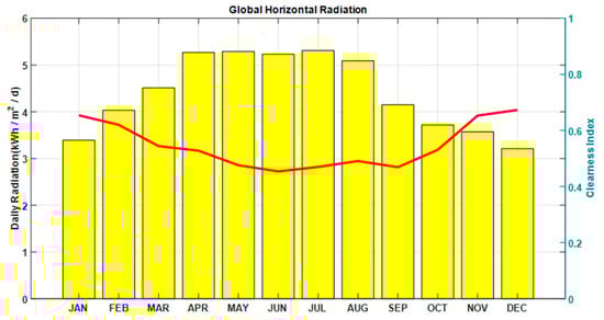
Figure 2.
Monthly solar radiation intensity and clearness index in a year. The left vertical coordinate is the daily average solar radiation intensity, and unit is kWh/m2/day. The right vertical coordinate is the clearness index, between 0 and 1.
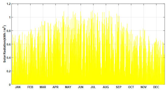
Figure 3.
The time sequence of solar radiation intensity in a whole year predicted by HOMER. The ordinate is solar radiation intensity and unit is kWh/m2.
3.5. The Character of Renewable Energy
Based on Section 3.3 and Section 3.4, the character of PV source was calculated, as shown in Table 3 and Table 4.
Table 3.
PV output power (kW) at each scenario and each time.
Table 4.
Probability at each scenario and time.
4. DR Model Considering Real-Time Tariff
In China, TOD tariff is the main measure of Demand Side Management (DSM). It started in the 1980s, and has now spread nationwide. Generally, it is divided into the three periods peak, flat and low, which correspond to high, medium and low prices, respectively. Real-time tariff is one of the vital indices of price type DR. Compared with incentive type DR, price type DR adjusts the running time of time-shifting load, which is friendlier to consumers. This method restrains consumers’ increasing demand and gives consumers economic benefits back at the same time. Thus, power supply corporations and consumers are willing to implement the policy.
4.1. Real-Time Tariff Model
The real-time tariff of moment i is []:
where Li is the load of moment i and P0 is the sales price without real-time price.
Using partial load to implementing real-time tariff requires setting a Customer Baseline Load (CBL), which is delimited according to customer’s historical load. If customer’s load does not exceed CBL, it follows the original tariff policy. The real-time tariff is only used on the exceeding CBL parts.
4.2. The Consumer Simulation
Users will adjust their consumption behavior all the time based on their real-time tariff, which optimizes the load curve. DR combined behavior model based on real-time tariff includes two cases, namely self-elasticity and cross-elasticity, which can be expressed as follows []:
where is the price at moment j after implementing the real-time tariff. and are the initial load at moments i and j. is the load after DR at moment i. E is the reward or punishment part for users changing their electricity consumption behavior. is the price elasticity of demand coefficient (PED), which reflects the sensitivity of changes in commodity DR to price changes in the market. When PED is the price self-elasticity of demand coefficient. When , PED is the cross-price elasticity of demand (CPED). CPED represents the sensitivity of a change in the demand for one commodity response to the price of another commodity, which can complement or replace each other. The PED and CPED values refer to the operation experience of foreign power market. It is considered that all the PED values of trough, flat and peak are −0.05, and the CPED values between trough and flat, trough and peak, flat and peak are 0.01, 0.012 and 0.016, respectively. Considering the actual electricity load in agriculture, we chose to only use PED rather than CPED because of its small numerical value.
4.3. Case Data
The load of agricultural users’ electricity consumption data in Gansu Province is shown in Table 5. Agricultural electricity time-of-use price, as shown in Table 6, is based on Gansu Grid Corporation (http://www.gs.sgcc.com.cn/).
Table 5.
Typical daily load of an agricultural user.
Table 6.
TOD tariff for agricultural electricity.
4.4. Case Study
According to the load data for each period, the real-time price based on user’s load can be calculated by Equation (14). The results are shown in Table 7.
Table 7.
The real-time price based on user’s load.
Treating the previous day load of the agricultural user as the load level of the real-time tariff, the user’s load response with the fully real-time tariff and the partial real-time tariff based on CBL are shown in Table 8 and Figure 4 according to Equation (15). It is assumed that the CBL-based partial real-time tariff will be executed at a 50% rate. L1 represents the user’s load response under the fully real-time tariff mechanism, and L2 represents the user’s load response under the partial real-time tariff mechanism based on CBL.
Table 8.
User’s load response with real-time price.
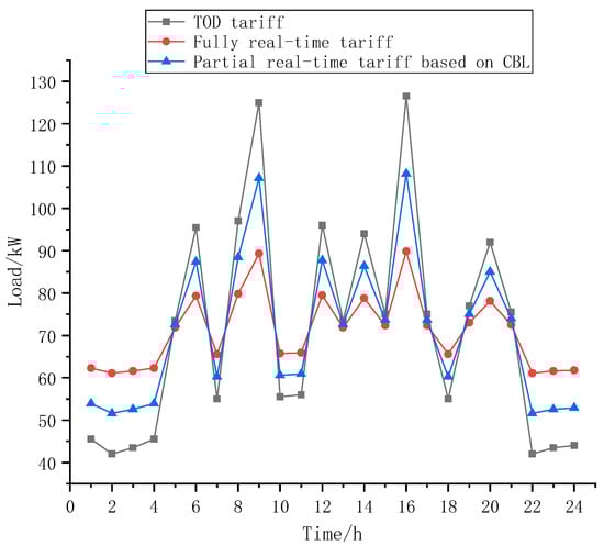
Figure 4.
User’s load response with real-time price.
Fully real-time tariff and CBL-based partial real-time tariff can reduce peak-trough load difference. The original peak-trough load difference is 84.5 kW, while the peak-trough load difference is 28.7 kW with real-time tariff. Based on CBL partial real-time tariff, the peak-trough load difference is 56.6 kW. The effect of load transfer under fully real-time tariff is more obvious.
5. Optimal Dispatching of Micro-Energy-Grid
5.1. Objective Function
We use the minimum comprehensive cost of the agricultural greenhouse in micro-energy-grid within 24 h as objective function. The comprehensive cost includes the purchase and sale cost , operation and maintenance cost , environmental cost and PV incomplete penalty cost . The objective function is [,]:
where is the probability of scenario s at moment t; and are the purchase and sale price at moment t respectively; and are the purchase and sell power from or to the grid in scenario s at moment t, and the latter should be a negative value; is the operation cost of type i equipment at moment t; is the power of type i equipment at moment t; is the operation cost of PV power generation equipment at moment t; and is the PV actual output power of scenario s at moment t. is the generating power of the CHP set at moment t, is the emission of the jth pollutant gas from CHP, is the sum of the environmental value and penalty of the jth pollutant gas, is the maximum PV output of scenario s at moment t, and is penalty costs for incomplete PV absorption.
5.2. Constraint Equation
5.2.1. Thermoelectric Power Balance Constraints
and are the charging and discharging power at moment t, where a positive value means the remaining energy stored in the battery from the grid or PV power generation, while a negative value represents the energy released from the battery to the electric load. and are the non-time-shifting load and time-shifting load at moment t, is the electric power required by ASHP at moment t, and is the heat-generating power of CHP at moment t. is the heating power of ASHP at moment t. and are the charging and discharging power at moment t, where a positive value represents the phase change heat storage device absorbs heat, while a negative value represents it releases heat. is the heat load at moment t.
5.2.2. Energy Conversion Element Constraints
Energy conversion elements in agricultural greenhouse of micro-energy-grid include MT, absorption heat pump, ASHP and PV power generation equipment, which should meet the inequality constraints of Equations (20)–(24).
where and are the maximum power of CHP generation and heat generation. and are the maximum power of ASHP consumption and heat generation. Equation (24) denotes the range of actual PV output power. is the maximum PV output value of scenario s at moment t.
5.2.3. Energy Storage Element Constraints
Energy storage elements include batteries and phase-change heat storage devices. SOC and SOH satisfy Equations (3) and (4). Moreover, they should also satisfy:
where Equations (25) and (26) are constraints on the energy storage capacity of storage elements. and are the minimum and maximum energy storage capacity of the battery. and are the minimum and maximum heat storage capacity of the phase change heat storage device. Equations (27)–(30) are constraints on charge and discharge heat power at moment t. and are the maximum allowable charge and discharge power of the battery, and is the maximum allowable charge or discharge power of the phase change heat storage device. and are two 0–1 variables, which limit batteries and phase change heat storage devices cannot charge or discharge at the same time.
Moreover, in a scheduling cycle, Equations (31) and (32) should be satisfied to ensure that the energy storage components are at the same state at the beginning and the end of the scheduling cycle. The consistency in each scheduling cycle should also be ensured.
5.2.4. Power Exchange Constraints with Distribution Network
To ensure the stability of power system in distribution network, power exchange with distribution network should satisfy the following constraints:
where is the purchase power of scenario s at moment t, which is a positive value; is the sale power of scenario s at moment t, which is a negative value; and are the maximum and minimum value of power exchange with distribution, respectively network; and is a 0–1 variable and restricts the simultaneous occurrence of purchasing and selling electricity with 1 representing purchasing electricity from the grid and 0 representing selling.
5.3. Parameter Settings
Our target is the micro-energy-grid of an agriculture greenhouse in a region of Gansu Province, China. The temperature inside and outside of a typical greenhouse is shown in Figure 5. The temperature inside the greenhouse is controlled at a constant temperature 25 °C. The data of the temperature outside the greenhouse were from National Meteorological Information Center of China. We put the data into Equation (8), and obtained the heat load of the greenhouse at each moment in a scheduling cycle. The heat transfer coefficients of the greenhouse film, wall and ground are 1.12, 0.62 and 0.24 W/(m2.k), respectively; the corresponding measures of area are 720, 170 and 640 m2; the air volume is 1360 m3; and the ventilation frequency is 1.2 times/h. Using 150 kWp PV cells, the PV output and its probability of each scenario in a typical day are shown in Table 3 and Table 4. Electric load is the sum of time-shifting load and non-time-shifting load. We considered 13 types of electric load objects in this study. Their time-shifting characteristics and the input time of non-time-shifting load at initial state from state grid science and technology project are shown in Table 9. Combining the above results, the PV output, thermal load, time-shifting load and non-time-shifting load in greenhouse are shown in Figure 6.
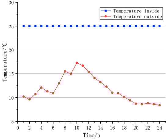
Figure 5.
The temperature inside and outside of a typical greenhouse.
Table 9.
Time-shifting characteristics and the input time of non-time-shifting load at initial state for 13 types of electric load.
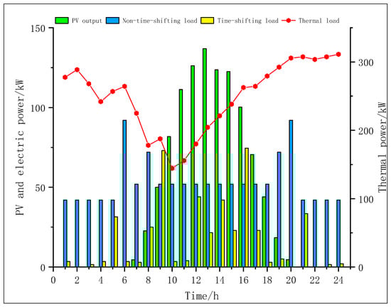
Figure 6.
The PV output and three loads in greenhouse.
The time-of-use tariff of agricultural electricity in Gansu power grid is shown in Table 10. The data were from Gansu Development and Reform Commission [].
Table 10.
Time-of-use tariff of agricultural electricity in Gansu.
Emission coefficients of gaseous pollutants and corresponding environmental costs are shown in Table 11.
Table 11.
Emission coefficients of gaseous pollutants and corresponding environmental costs.
The greenhouse includes microturbine, absorption heat pump, ASHP, storage battery, phase change heat storage device and PV power generation equipment. The upper and lower operating limits, conversion coefficients, capacity and operating costs of the equipment are shown in Table 12.
Table 12.
Equipment parameters in micro-energy-grid.
We selected five cases as examples to analyze. TOD tariff and non-time-shifting load are used in Case 1 and Case 4, TOD tariff and time-shifting load are used in Case 2 and Case 5, and real-time price and time-shifting load are used in Case 3. The difference between Case 1 and Case 4 or Case 2 and Case 5 is whether to allow using excess electricity to get profit from the grid. The specific setup for each case is shown in Table 13.
Table 13.
The specific setup for each case.
5.4. Results
The day-ahead optimal scheduling in this paper is a 0–1 mixed integer linear programming (MIP) problem. GAMS is an optimization software using CPLEX to solve the MIP problem. The scheduling step size is 1 h and the scheduling cycle is 24 h of a day. Figure 7 shows the result of optimal dispatch of electric power in five cases. The positive value represents the power provided by PV, CHP, grid and storage battery. The negative value represents the power consumed by time-shifting load, non-time-shifting load, ASHP power, surplus power grid and battery charging. Figure 8 shows the optimal dispatch result of thermal power in five cases. The positive value represents the provided thermal power, including waste heat recovery in CHP, heat generation by ASHP and heat release by phase change heat storage device. The negative value represents the consumption of thermal power, including heat load and heat absorption by phase change heat storage device.
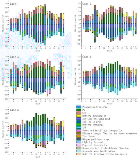
Figure 7.
The result of optimal dispatch of electric power in five cases.
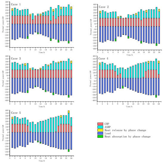
Figure 8.
The optimal dispatch result of thermal power in five cases.
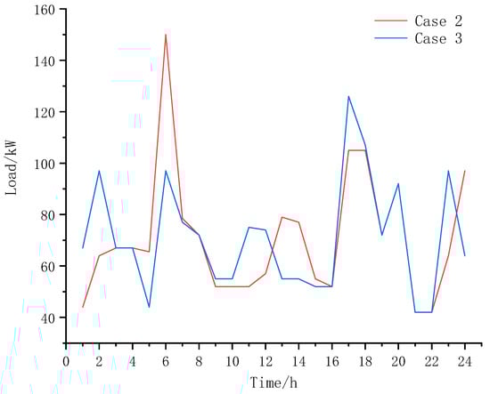
Figure 9.
The load response of TOD tariff and real-time price.
- When daylight is sufficient, comparing Cases 3 and 4, we found that the power load is borne by PV whether or not it is permissible the sale of electricity to micro-energy-gird. In Case 3, another source of power load is CHP. However, in Case 4, the source of power load is purchasing from grid and electricity can be converted into heat.
- The introduction of time-shifting loads can make the micro-energy-grid have the characteristics of load transfer. Comparing Cases 1 and 2, the time-shifting loads were transferred from high electricity price at 16:00 to low electricity price at 6:00, which made the load curve optimized.
The input time schedule of time-shifting load is shown in Table 14. Cases 2 and 3 are selected to compare the load response to TOD tariff and real-time price, as shown in Figure 9. Case 2 uses the current TOD tariff and Case 3 calculates the dynamic real-time tariff. Combining with Figure 8, it can be seen that both TOD and real-time tariffs can transfer load to the night trough. However, compared with real-time tariff, TOD tariff produces new load peaks at 6:00, thus the effect of real-time tariff to reduce peak–trough difference is better.
Table 14.
The input time schedule of time-shifting load.
The electricity purchasing and selling status, PV absorption status and integrated operation cost in five cases are shown in Table 15.
Table 15.
The electricity purchasing and selling status, PV absorption status and synthetic operation cost in five cases.
In Table 15, the following can be seen:
- In Cases 1–3, PV has been completely eliminated, because it allows the sale of surplus power from micro-energy-grid to distribution grid. Cases 4 and 5 can eliminate 92.97% and 95.88% of PV energy, respectively, without selling surplus power, but the phenomenon of light abandonment still can be curbed.
- Compared with Case 1, Cases 2 and 3 reduced the synthesized operation cost by 43.4% and 56.5%, respectively, which indicates that a reasonably working DR scheme can reduce the synthesized operation cost of a greenhouse.
6. Conclusions
Based on the study, we found the following:
- Selling electricity from the micro-energy-grid to power grid has great economic benefits and supporting environmental benefits.
- The day-ahead dispatch of time-shifting load has a great impact on the cost of electricity consumption in agricultural greenhouses.
- Real-time tariff has a good effect on peak cutting and trough filling; it also can reduce the electricity cost of an agricultural greenhouse to a certain level.
Author Contributions
Conceptualization, Y.J. and M.J.; methodology, Y.J.; software, M.J.; validation, Y.J. and J.Y.; formal analysis, Y.J.; investigation, M.J.; resources, Y.J.; data curation, M.J.; writing—original draft preparation, M.J.; writing—review and editing, J.W.; visualization, J.Y. and D.L.; supervision, Y.J.; project administration, Y.J. and K.S.; and funding acquisition, Y.J., M.D. and H.Z.
Funding
This paper is supported by Open Fund of FX83-18-0022018 year Beijing Key Laboratory of Demand Side Multi-Energy Carriers Optimization and Interaction Technique (No.YDB51201801084), the National Natural Science Foundation of China (Grant No. 51707196) and the State Key Laboratory of Alternate Electrical Power System with Renewable Energy Sources (Grant No. LAPS18015).
Acknowledgments
Yuntao Ju and Dezhi Li also belong to Beijing Key Laboratory of Demand Side Multi-Energy Carriers Optimization and Interaction Technique, Beijing 100192, China. Mingyu Dong and Kun Shi also belong to China Electric Power Research Institute, Haidian District, Beijing100192, China.
Conflicts of Interest
The authors declare no conflict of interest.
References
- Jin, H. A new principle of synthetic cascade utilization of chemical energy and physical energy. Sci. China Ser. E Technol. Sci. 2005, 48, 163–179. [Google Scholar] [CrossRef]
- Kang, C.; Chen, Q.; Xia, Q. Prospects of Low-Carbon Electricity. Power Syst. Technol. 2009, 33, 1–7. [Google Scholar]
- Cheng, Y.; Zhang, N.; Kang, C.; Kirschen, D.; Zhang, B. Research Framework and Prospects of Low-carbon Multiple Energy Systems. Proc. CSEE 2017, 37, 4060–4069. [Google Scholar]
- Liu, X.; Wu, J.; Jenkins, N.; Bagdanavicius, A. Combined analysis of electricity and heat networks. Appl. Energy 2016, 162, 1238–1250. [Google Scholar] [CrossRef]
- Geidl, M.; Koeppel, G.; Favre-Perrod, P.; Klockl, B.; Andersson, G.; Frohlich, K. Energy hubs for the future. Power Energy Mag. IEEE 2007, 5, 24–30. [Google Scholar] [CrossRef]
- Wang, Y.; Zhang, N.; Kang, C. Review and Prospect of Optimal Planning and Operation of Energy Hub in Energy Internet. Proc. CSEE 2015, 35, 5669–5681. [Google Scholar]
- Gan, L.; Chen, Y.; Liu, Y.; Xiong, W.; Tang, L.; Pan, Z.; Guo, Q. Coordinative optimization of multiple energy flows for microgrid with renewable energy resources and case study. Electr. Power Autom. Equip. 2017, 37, 275–281. [Google Scholar]
- Bao, Z.; Zhou, Q.; Yang, Z.; Yang, Q.; Xu, L.; Wu, T. A Multi Time-Scale and Multi Energy-Type Coordinated Microgrid Scheduling Solution—Part II: Optimization Algorithm and Case Studies. IEEE Trans. Power Syst. 2015, 30, 2267–2277. [Google Scholar] [CrossRef]
- Nguyen, D.T.; Negnevitsky, M.; de Groot, M. A comprehensive approach to Demand Response in restructured power systems. In Proceedings of the Australasian Universities Power Engineering Conference, Christchurch, New Zealand, 5–8 December 2010; p. 6. [Google Scholar]
- Cui, Y.; Zhang, H.; Zhong, W.; Zhao, Y.; Wang, Z.; Xu, B. Day-ahead Scheduling Considering the Participation of Price-based Demand Response & CSP Plant in Wind Power Consumption. Power Syst. Technol. 2019, 1–9. [Google Scholar]
- Zhou, B.; Huang, T.; Zhang, Y. Reliability Analysis on Microgrid Considering Incentive Demand Respons. Autom. Electr. Power Syst. 2017, 41, 70–78. [Google Scholar]
- Mao, Y. Demand Response Model of Electric-Gas Integrated Energy Ecosystem Based on Double-Level Joint Optimization. Smart Power 2018, 46, 18–25. [Google Scholar]
- Zhang, Y. Optimal Dispatch of Integrated Electricity-Natural Gas System Considering Demand Response and Dynamic Natural Gas Flow. AEPS 2018, 42, 1–10. [Google Scholar]
- Zhang, Z. Optimization Hotspot Region Based Integrated Demand Response Model of User-side Combined Heat and Power Unit. Electr. Power Constr. 2018, 39, 20–27. [Google Scholar]
- Xia, S.; Zhang, Q.; Hussain, S.; Hong, B.; Zou, W. Impacts of integration of wind farms on power system transient stability. Appl. Sci. 2018, 8, 1289. [Google Scholar] [CrossRef]
- Wang, F.; Yu, Y.; Zhang, Z.; Li, J.; Zhen, Z.; Li, K. Wavelet decomposition and convolutional LSTM networks based improved deep learning model for solar irradiance forecasting. Appl. Sci. 2018, 8, 1286. [Google Scholar] [CrossRef]
- Ju, Y.; Wang, J.; Ge, F.; Lin, Y.; Dong, M.; Li, D.; Shi, K.; Zhang, H. Unit Commitment Accommodating Large Scale Green Power. Appl. Sci. 2019, 9, 1611. [Google Scholar] [CrossRef]
- Li, C.; Yun, J.; Ding, T.; Liu, F.; Ju, Y.; Yuan, S. Robust Co-optimization to energy and reserve joint dispatch considering wind power generation and zonal reserve constraints in real-time electricity markets. Appl. Sci. 2017, 7, 680. [Google Scholar] [CrossRef]
- Duan, J.; Wang, X.; Gao, Y.; Yang, Y.; Yang, W.; Li, H.; Ehsan, A. Multi-Objective Virtual Power Plant Construction Model Based on Decision Area Division. Appl. Sci. 2018, 8, 1484. [Google Scholar] [CrossRef]
- Zhao, Y.; Che, Y.; Wang, D.; Liu, H.; Shi, K.; Yu, D. An Optimal Domestic Electric Vehicle Charging Strategy for Reducing Network Transmission Loss While Taking Seasonal Factors into Consideration. Appl. Sci. 2018, 8, 191. [Google Scholar] [CrossRef]
- Chen, Z. Economic Dispatch Optimization of Integrated Energy System in Multi Energy Flow Area. Master’s Thesis, Xi’an University of Technology, Xi’an, China, 2018. [Google Scholar]
- Zhang, S.; Cheng, H.; Zhang, L.; Bazargan, M.; Yao, L. Probabilistic evaluation of available load supply capability for distribution system. IEEE Trans. Power Syst. 2013, 28, 3215–3225. [Google Scholar] [CrossRef]
- Wang, J. Research on Energy Dispatch Day-ahead Schedule for Household Microgrids. Electr. Meas. Instrum. 2013, 50, 81–86. [Google Scholar]
- Zhou, Z. Calculation of Heating Load in Greenhouse and Selection of Common Temperature Supplementary Ways. Vegetable 2004, 41–43. [Google Scholar]
- Xue, D. Calculating Heating Load of Greenhouse. Agric. Jilin 2016, 58. [Google Scholar]
- Chen, C.; Wu, W.; Zhang, B.; Qin, J.; Guo, Z. An Active Distribution System Reliability Evaluation Method Based on Multiple Scenarios Technique. Proc. CSEE 2012, 32, 67–73. [Google Scholar]
- Razali, N.M.M.; Hashim, A.H. Backward reduction application for minimizing wind power scenarios in stochastic programming. In Proceedings of the 2010 4th International Power Engineering and Optimization Conference (PEOCO), Shah Alam, Selangor, Malaysia, 23–24 June 2010; pp. 430–434. [Google Scholar]
- Zhou, L. Research on User Real Time Pricing Mechanism under the Condition of Smart Grid. Master’s Thesis, North China Electric Power University, Beijing, China, 2015. [Google Scholar]
- Aalami, H.A.; Moghaddam, M.P.; Yousefi, G.R. Demand response modeling considering Interruptible/Curtailable loads and capacity market programs. Appl. Energy 2010, 87, 243–250. [Google Scholar] [CrossRef]
- Wang, W. Optimization of the micro energy grid of PV intelligent agricultural greenhouse based on time-shifting agricultural load. J. China Agric. Univ. 2018, 23, 160–168. [Google Scholar]
- Xu, H. Optimization dispatch strategy considering renewable energy consumptive benefits based on “source-load-energy storage” coordination in power system. Power Syst. Prot. Control 2017, 45, 18–25. [Google Scholar]
- Wang, J. Notice on the Adjustment of the Grid Value-Added Tax Rate to Reduce the General Industrial and Commercial Electricity Price. Available online: http://fzgg.gansu.gov.cn/content/2019-04/43589.html (accessed on 19 April 2019).
© 2019 by the authors. Licensee MDPI, Basel, Switzerland. This article is an open access article distributed under the terms and conditions of the Creative Commons Attribution (CC BY) license (http://creativecommons.org/licenses/by/4.0/).