The Complex Dynamic Locomotive Control and Experimental Research of a Quadruped-Robot Based on the Robot Trunk

Featured Application

This paper focuses on the dynamic pacing gait planning and control of hydraulic quadruped robot. The performance of robot has been improved. As an experimental platform, the research of the robot on complex terrain can be completed in the future.

Abstract

The research of quadruped robots is fundamentally motivated by their excellent performance in complex terrain. Maintaining the trunk moving smoothly is the basis of assuring the stable locomotion of the robot. In this paper we propose a planning and control strategy for the pacing gait of hydraulic quadruped robots based on the centroid. Initially, the kinematic model between the single leg and the robot trunk was established. The coupling of trunk motion and leg motion was elaborated on in detail. Then, the real-time attitude feedback information of the trunk was considered, the motion trajectory of the trunk centroid was planned, and the foot trajectory of the robot was carried out. Further, the joint torques were calculated that fulfillment minimization of the contact forces. The position and attitude of the robot trunk were adjusted by the presented controller. Finally, the performance of the proposed control framework was tested in simulations and on a robot platform. By comparing the attitude of the robot trunk, the experimental results show that the trunk moved smoothly with small-magnitude by the proposed controller. The stable dynamic motion of the hydraulic quadruped robot was accomplished, which verified the effectiveness and feasibility of the proposed control strategy.

1. Introduction

Quadruped robots have wide application prospects in complex environments, since they have high power density, strong load capacity, and great mobility and flexibility [1,2,3,4]. They are superior to tracked robots and wheeled robots, due to the advantage of better terrain adaptability. The Bigdog robot developed by Boston Dynamic in 2008 is the representative of the hydraulic quadruped robot [5]. Bigdog has good adaptability and stability, and can adapt to complex and dangerous environments, such as mountains, jungles, beaches, swamps, ice and snow. Since then, hydraulic quadruped robots have become a popular research topic because of their excellent obstacle-crossing and anti-interference ability in complex environments [6,7,8], and some momentous achievements have been made in recent years. For instance, Boston Dynamic’s Alpha Dog [9], Cheetah [10], Spot [11] and Spotmini [12], ETH Zurich’s ANYmal [13], the Italian Institute of Technology’s HyQ [14], MiniHyQ [15] and HyQ2Max [16], and Shandong University’s SCalf-I [17] and SCalf-II [18].

Quadrupeds in nature can choose different gaits to complete their movements according to their purposes and topographic information [2]. The motion modes of quadruped robots are inspired by quadruped animals [19]. The trotting gait is a common gait in quadruped mammals. Therefore, the trotting gait of hydraulic quadruped robots is one of the research hotspots. Moro FL et al. [20] proposed a method to directly apply the motion characteristics of horses to a quadruped robot. The foot trajectory was generated by a set of four kinematic motion primitives, and the stable, valid and effective walking and trotting gait of a quadruped robot was realized. Chung JW et al. [21] successfully tested the trotting gait of a quadruped robot by using the dynamic model of virtual biped gait. Havoutis I et al. [22] designed a gait controller for trotting gait, and the problem of force balance in the process of robotic motion was solved by using active compliance control. Cai RB et al. [23] proposed a time and attitude control method, which divides the control of quadruped robot into gait control and attitude control. Gehring et al. [24] proposed a controller that can switch between walking trot and running trot.

However, while a hydraulic quadruped robot moves with trot gait, its two swinging legs often fail to touch the ground at the same time. In that case, the robot trunk will rotate obliquely around the supporting leg, since the first landing leg has a great impact on the trunk. The turning moment around the supporting diagonal line will be generated. He et al. [25] used the starting posture to weaken the adverse effects of overturning moment. Xie et al. [26] verified that the overturning torque was caused by the forward swing joints at the hips of the standing legs, and proposed an attitude control method to balance overturning moment by using the hip side-sway joint moment. Nonetheless, these conclusions have not been validated on the robot platform, nor can they fundamentally solve the problem of robot turnover. Moreover, most of the current research efforts focus on the simple trot gait, and less on the more complex dynamic gait. In this context, the gait selection of robots in complex terrain has certain limitations.

In addition, the hydraulic quadruped robot is a strongly coupled nonlinear system. In the process of robot locomotion, the trunk is always in a bumpy state and often affected by unpredictable factors [27]. Boussema et al. [28] proposed a posture recovery strategy based on a feasible impulse group, and the effectiveness of this method was verified when the Cheetah-3 robot was disturbed by external disturbances. A control strategy based on four three-dimensional spring dampers was proposed by Tran et al. [29], and the rotational disturbance control of quadruped walking robot under unknown terrain conditions was implemented. A gait generator based on CPGs modulated by vestibular feedback was proposed by Fukui T et al. [30]. The bio-inspired robot robustly ran with an emergent gallop while stepping on and over several types of unperceived obstacles. Park et al. [31] presented a feedback controller, which allowed the robot to change its gait parameters according to terrain information. Due to the external disturbance and the real-time change of trunk position and attitude, there is an enormous gap between the theoretical and practical results of the robot driving functions. Hence, for a hydraulic quadruped robot, the position and posture of the robot trunk must be divided into the individual legs. However, the position and attitude information of the trunk in the process of robotic motion is not taken into account in the above methods.

This paper focuses on the complex dynamic gait control problem of the hydraulic quadruped robot. On the premise of guaranteeing the motion speed of the robot and in order to improve the stability of the robot, a controller for the pacing gait of the hydraulic quadruped robot is proposed. Unlike previous works, we derived our controller from the centroid of the robot trunk. Firstly, we specifically stated the relationship between the joint of the leg and the attitude information of the robot trunk. Secondly, the trajectory of the centroid of the trunk was planned. Then, we extended the method to avoid the instability of the robot when its feet touch the ground. A controller based on centroid of the trunk was designed, which can adjust the driving function in real time according to the position and attitude of the trunk. Lastly, the cyclic and stable pace gait in a simulation and on an actual robot platform were tested, which testifies to the validity and feasibility of the proposed control strategy.

For the sake of establishing this controller, our paper is organized as follows. Section 2 depicts the mechanical structure of the hydraulic quadruped robot, and establishes the kinematic model of the robot. Section 3 describes the trajectory planning for the centroid of the robot trunk. Section 4 is the design of pace-gait controller for the hydraulic quadruped robot. Section 5 verifies the control algorithm by simulation. Section 6 introduces our hydraulic quadruped robot experimental platform and reports the experimental results. Finally, Section 7 draws the conclusions of the full paper.

2. The Modeling of the Hydraulic Quadruped Robot

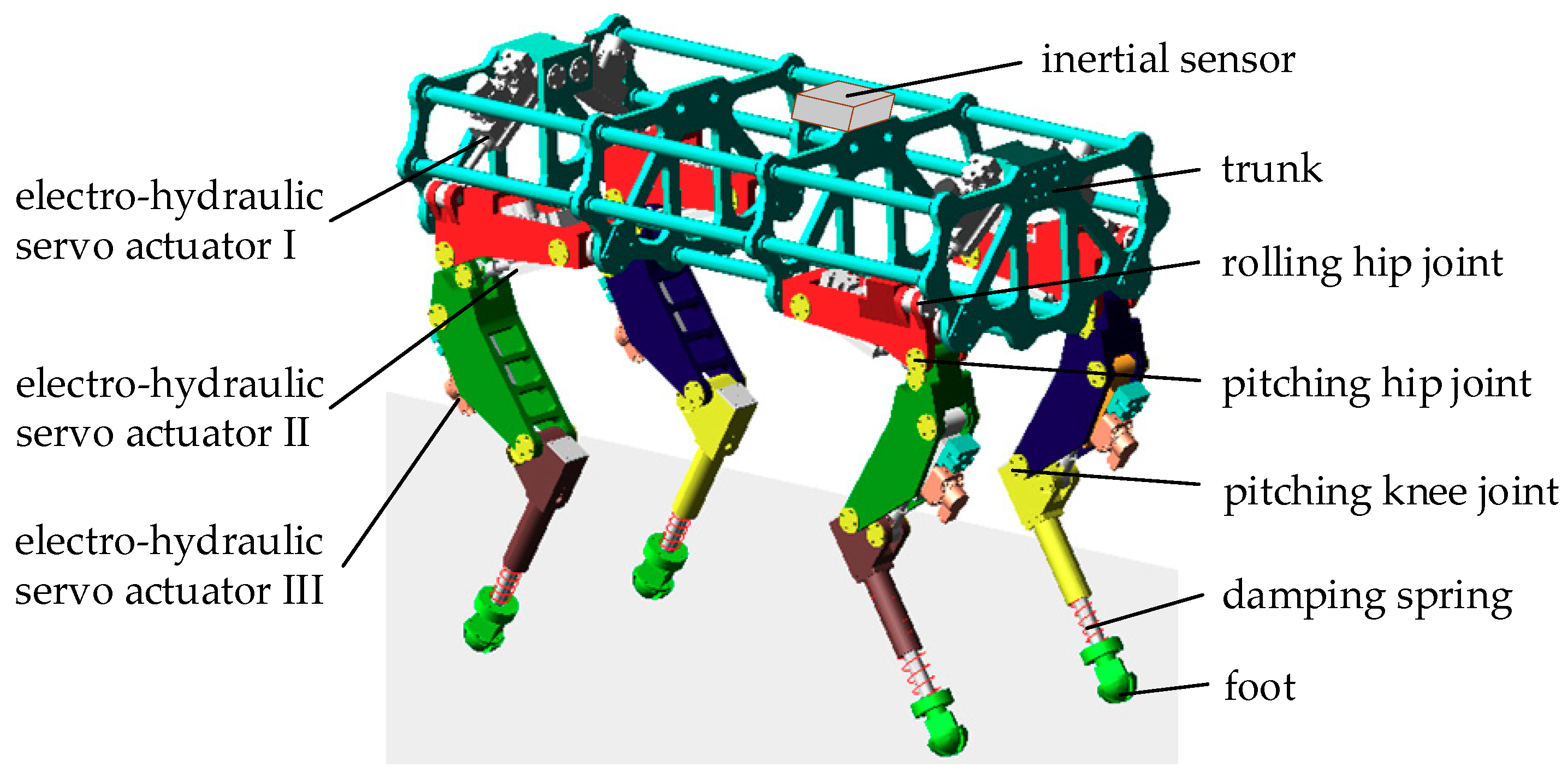
2.1. The Mechanical Structure of the Hydraulic Quadruped Robot

The mechanical structure of a hydraulic quadruped robot consists of a trunk and four legs, as shown in Figure 1. An inertial sensor for real-time attitude detection of the trunk is fixed on the robot trunk. The hydraulic quadruped robot has eighteen degrees of freedom, which are twelve joint degrees of freedom and six trunk degrees of freedom. There are generally three active joints of each leg, which are the rolling hip joint, the pitching hip joint and the pitching knee joint. The twelve active joints are driven by the identical electro-hydraulic servo actuator.

Hydraulic quadruped robot is a mobile platform. The motion of robot is primarily realized by the movement of trunk and swing legs. In order to analyze the reasons of the change of the posture of the robot trunk, the kinematic characteristics of the robot and the force of the supporting legs to the trunk should be analyzed. The kinematic model consists of two parts: one is the relationship between the foothold position and the joint angle of a single leg; the other is the relationship between single leg and the robot trunk.

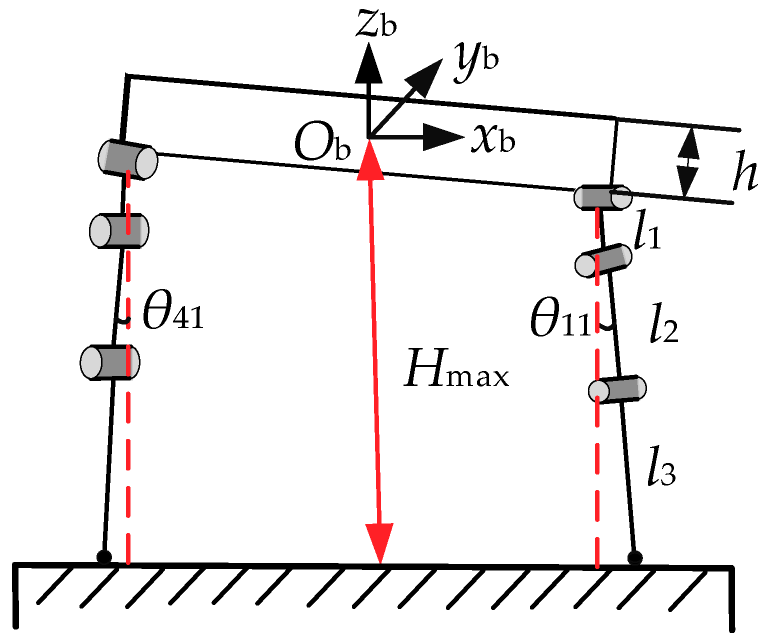
2.2. Kinematic Modeling

As shown in Figure 2, the kinematic model of the robot is established based on the improved D-H (Hartenbery) parameter method. The robot requires four coordinate frames. They are the reference coordinate frame, the torso coordinate frame, the transitional coordinate frame and the joint coordinate frame. The reference coordinate frame {O_w} is a coordinate system representing all forces, displacements and velocities, also known as the inertial coordinate system. {O_w} is fixed on the ground. x_w points to the forward direction of the robot; z_w is perpendicular to the trunk and points in the opposite direction to the ground; and y_w is determined by the right-hand rule. The origin of the torso coordinate frame {O_b} is located in the geometric center of the robot trunk. The axis direction of torso coordinate frame is the same as that of frame {O_w}. The transitional coordinate frames {O_i0} are fixed on the corners of the trunk. The subscript i is the serial number of four robotic legs (i = 1, 2, 3 and 4), representing the right foreleg (RF), left foreleg (LF), left hindleg (LH) and right hindleg (RH), respectively. The joint coordinate frames {O_ij} are fixed on the joints of the robot. The subscript j is the serial number of joints (j = 1, 2, 3 and 4), representing the horizontal pendulum joint, hip joint, knee joint and foot joint, respectively. 2a is the length of the robot trunk, 2b is the width of the robot trunk and h is the height of the robot trunk. l₁ is the length of the link rod between the trunk and thigh, l₂ is the length of the thigh and l₃ is the length of the shank. θ_i1, θ_i2 and θ_i3 are the rolling hip joint angle, pitching hip joint angle and pitching knee joint angle, respectively.

Since the mechanical structure of the four legs is identical, the coordinate frame established according to the D-H rule of the four legs is exactly the same. Hence the transformation matrix from the foot coordinate frame {O_i4} to the transitional coordinate frame {O_i0} of each leg is identical. The transformation matrix ⁰T_i4 can be expressed as:

$${}^0{\mathit{T}}_{i4}=\left[\begin{array}{cccc}{c}_1{c}_{23}& -c_1{s}_{23}& s_1& {}^{0}p{}_{ix}\\ s_1{c}_{23}& -s_1{s}_{23}& -c_1& {}^{0}p{}_{iy}\\ s_{23}& c_{23}& 0& {}^{0}p{}_{iz}\\ 0& 0& 0& 1\end{array}\right]$$

(1)

where s₂₃ = sin(θ₂ + θ₃), c₂₃ = cos(θ₂ + θ₃), s₁ = sinθ₁ and c₁ = cosθ₁. ⁰p_ix, ⁰p_iy and ⁰p_iz represent the x-coordinate, y-coordinate and z-coordinate of the foot in the corresponding transitional coordinate frame, respectively.

The position of the foot of the hydraulic quadruped robot in the transitional coordinate frame ⁰p_ie = {⁰p_ix ⁰p_iy ⁰p_iz 1}^T is given by:

$$\{\begin{array}{l}{}^{0}p{}_{ix}=c_1\left(l_1+l_2{c}_2+l_3{c}_{23}\right)\\ {}^{0}p{}_{iy}=s_1\left(l_1+l_2{c}_2+l_3{c}_{23}\right)\\ {}^{0}p{}_{iz}=l_2{s}_2+l_3{s}_{23}\end{array}$$

(2)

Based on forward kinematic analysis, the transformation matrix from {O_i0} to {O_b} of four legs is then found:

$${}^{\mathrm{b}}\mathit{T}{}_{i0}=\left[\begin{array}{cccc}0& 0& 1& \alpha a\\ 0& 1& 0& \beta b\\ -1& 0& 0& -h\\ 0& 0& 0& 1\end{array}\right]$$

(3)

where α and β are symbolic signs, which are defined as follows:

$$\alpha =\{\begin{array}{cc}1& i=1,2\\ -1& i=3,4\end{array}$$

(4)

$$\beta =\{\begin{array}{cc}1& i=2,4\\ -1& i=1,3\end{array}$$

(5)

The inverse kinematic analysis is significant for gait planning and motion control of quadruped robots. Since the forelegs of the hydraulic quadruped robot are elbow joints and the hind legs are knee joints [32,33], the joint variables θ_i2 and θ_i3 obtained based on inverse kinematic are different. The joint angles of the hydraulic quadruped robots are as Equation (5).

$$\{\begin{array}{l}{\theta }_{i1}=\arctan \left(\frac{{}^{0}p{}_{iy}}{{}^{0}p{}_{ix}}\right)\\ {\theta }_{i3}=\pm \arccos \frac{m^2+{}^{0}p{{}_{iz}}^2-l_2{}^2-l_3{}^2}{2l_2{l}_3}\\ {\theta }_{i2}=\pm \arccos \frac{(l_2+l_3{c}_3)m+l_3{s}_3{}^{0}p{}_{iz}}{l_2{}^2+l_3{}^2+2l_2{l}_3{c}_3}\end{array}$$

(6)

where m is defined as:

$$m=\sqrt{{}^{0}p{{}_{ix}}^2+{}^{0}p{{}_{iy}}^2}-l_1$$

(7)

Obviously, for RF and LF (i = 1, 2) of a hydraulic quadruped robot, θ_i2 and θ_i3 are positive. On the contrary, for LH and RH (i = 3, 4) of a hydraulic quadruped robot, θ_i2 and θ_i3 are negative.

If given the coordinate of a foot in the torso coordinate frame {O_b}, the joint angles of quadruped robot legs could be solved by Equations (3) and (6).

Jacobian matrix is a mapping of foot velocity and joint velocity, which can be derived from Equations (1) and (3).

$$\mathit{J}=\left[\begin{array}{ccc}0& l_2{c}_2+l_3{c}_{23}& l_3{c}_{23}\\ c_1(l_1+l_2{c}_2+l_3{c}_{23})& -s_1(l_2{s}_2+l_3{s}_{23})& -l_3{s}_1{s}_{23}\\ -s_1(l_1+l_2{c}_2+l_3{c}_{23})& s_1(l_2{s}_2+l_3{s}_{23})& l_3{c}_1{s}_{23}\end{array}\right]$$

(8)

If the joint angles in the joint space θ_i = [θ_i1 θ_i2 θ_i3]^T are known, the motion velocities of the foot in three directions along the torso coordinate frame {O_b} can be obtained according to Jacobian matrix using:

$${}^{\mathrm{b}}\mathit{V}{}_i={}^{\mathrm{b}}\dot{\mathit{p}}{}_i=\mathit{J}({\theta }_i){\dot{\mathit{\theta }}}_i$$

(9)

where ^bV_i and ^bp_i represent the velocity vector and position vector of the foot in the torso coordinate frame, respectively.

Conversely, the joint angular velocity in joint space can be solved from the velocity of the foot and the inverse of Jacobian matrix.

$${\dot{\mathit{\theta }}}_i={\mathit{J}}^{-1}({\theta }_i){}^{\mathrm{b}}\mathit{V}={\mathit{J}}^{-1}({\theta }_i){}^{\mathrm{b}}\dot{\mathit{p}}{}_i$$

(10)

where

$${\mathit{J}}^{-1}=\left[\begin{array}{ccc}0& c_1/(l_1+l_2{c}_2+l_3{c}_{23})& s_1/(l_1+l_2{c}_2+l_3{c}_{23})\\ s_{23}/(l_2{s}_3)& s_1{c}_{23}/(l_2{s}_3)& -c_1{c}_{23}/(l_2{s}_3)\\ -(l_2{s}_2+l_3{c}_{23})/(l_2{l}_3{s}_3)& -s_1(l_2{c}_2+l_3{c}_{23})/(l_2{l}_3{s}_3)& c_1(l_2{c}_2+l_3{c}_{23})/(l_2{l}_3{s}_3)\end{array}\right]$$

(11)

3. Trajectory Planning for Quadruped Robot

3.1. Trajectory Generation of Trunk Centroid

The motion of robot trunk has an important influence on the stability of a hydraulic quadruped robot. The position of the trunk is p_b = (x_b, y_b, z_b). The centroid trajectories of the trunk with bipedal support and quadruped support are designed separately. When the robot is supported by two feet, the centroid coordinate of the robot trunk is (x_bw (t), z_bw (t)). When the robot is supported by four feet, the centroid coordinate of the robot trunk is (x_bp(t), z_bp(t)).

3.1.1. Horizontal Position Planning of Robot Trunk

The horizontal displacements of the robot trunk centroid x_bw (t) and x_bp(t) are expressed by cubic polynomials as follows:

$$\{\begin{array}{ll}{x}_{\mathrm{bw}}(t)=d_0+d_{1}t+d_2{t}^2+d_3{t}^3& 0\le t\le T_{\mathrm{m}}\\ x_{\mathrm{bp}}(t)=c_0+c_{1}t+c_2{t}^2+c_3{t}^3& T_{\mathrm{m}}\le t\le T\end{array}$$

(12)

where T_m is the period time of the swing phase, T is the motion cycle of the hydraulic quadruped robot and t is the time.

According to (12), the range of t during quadruped support phase is from T_m to T. The trajectory of the centroid of the trunk should be continuous during the motion of the robot. It is mainly manifested in two aspects. The horizontal displacement and velocity of the trunk centroid at the beginning of the quadruped support phase coincide with their values at the end of the bipedal support phase. The attitude angle and angular velocity of the trunk centroid at the beginning of the bipedal support phase are consistent with those of the trunk centroid at the end of the quadruped support phase. The constraints are as follows:

$$\{\begin{array}{l}{x}_{\mathrm{bw}}(T_{\mathrm{m}})=x_{\mathrm{bp}}(0)\hfill \\ {\dot{x}}_{\mathrm{bw}}(T_{\mathrm{m}})={\dot{x}}_{\mathrm{bp}}(0)\hfill \\ x_{\mathrm{bw}}(0)=S_{\mathrm{w}0}\hfill \\ x_{\mathrm{bp}}(T)=\frac{S}{2}-S_{\mathrm{w}0}\hfill \\ {\dot{x}}_{\mathrm{bw}}(0)={\dot{x}}_{\mathrm{bp}}(T)\hfill \end{array}$$

(13)

where S_w0 is the position of the robot trunk centroid at the beginning of the bipedal support phase, and S is the stride length.

3.1.2. Vertical Position Planning of Robot Trunk

In the process of a robot’s motion, the vertical displacements of robot trunk centroid z_bw (t) and z_bp (t) are fixed values, which are as follows:

$$\{\begin{array}{cc}{z}_{\mathrm{bw}}(t)=H_{\mathrm{bz}}& 0\le t\le T_{\mathrm{m}}\\ z_{\mathrm{bp}}(t)=H_{\mathrm{bz}}& T_{\mathrm{m}}\le t\le T\end{array}$$

(14)

where H_bz is the height of the robot trunk.

If H_bz is too small, the force arm of the robot trunk centroid relative to the knee joint will be increased, hence the torque of the knee joint will be increased. Taking the two right landing legs (RF and RH) of the hydraulic quadruped robot as an example, the structure diagram of the robot is illustrated in Figure 3. In order to avoid the singularity bit-type of the robot, the maximum height of H_bz is:

$$H_{\max }=\frac{1}{2}\left[h\cos q_2+\left(l_1+l_2+l_3\right)\left(\cos {\theta }_{11}+\cos {\theta }_{41}\right)\right]$$

(15)

where q₂ is the pitch angle of the robot trunk. Due to the error between the actual robot structure and the theoretical model, the height of the center of mass of the trunk is generally 0.8 times of H_max.

Similarly, due to the symmetry of the structure of the hydraulic quadruped robot, while the robot is supported by four legs, the height of the trunk centroid is half of the total height of the two diagonally supported legs.

3.2. Foot Trajectory Planning of Quadruped Robot

Each leg of the hydraulic quadruped robot has three degrees of freedom, according to the above kinematic analysis, the joint trajectories can be calculated from the foot trajectories. The position of the robot foot is affected by the attitude of the trunk and the angle of the joint. The foot trajectory should not only meet the requirement of minimizing the contact force between the ground and the foot, but also ensure that the contact velocity of the foot is zero. Up to now, a variety of foot trajectory planning methods have been proposed, such as compound cycloid trajectory [34], modified compound cycloid trajectory [35,36], quintic polynomial curve trajectory [37], sine function trajectory [38], a combination trajectory of cubic polynomial and straight line trajectories [17] and elliptical trajectory [39]. However, the disturbance of the robot trunk is not considered in the above methods.

After comparing the various foot trajectory planning methods mentioned above, for this paper, the cycloid trajectory planning method proposed in reference [40] was decided on. The trajectory equations can be written as:

$$\{\begin{array}{ll}{p}_x=S\left(\frac{t}{T_{\mathrm{m}}}-\frac{1}{2\mathsf{\pi }}\sin (2\mathsf{\pi }\frac{t}{T_{\mathrm{m}}})\right)-\frac{S}{2}& 0\le t\le T_{\mathrm{m}}\\ p_y=0& 0\le t\le T_{\mathrm{m}}\\ p_z=2H\left[\frac{t}{T_{\mathrm{m}}}-\frac{1}{4\mathsf{\pi }}\sin (4\mathsf{\pi }\frac{t}{T_{\mathrm{m}}})\right]& 0\le t\le \frac{T_{\mathrm{m}}}{2}\\ p_z=2H\left[1-\frac{t}{T_{\mathrm{m}}}+\frac{1}{4\mathsf{\pi }}\sin (4\mathsf{\pi }\frac{t}{T_{\mathrm{m}}})\right]& \frac{T_{\mathrm{m}}}{2}\le t\le T_{\mathrm{m}}\end{array}$$

(16)

where H is the maximum height of the foot, p_x, p_y and p_z represent the horizontal displacement, lateral displacement and vertical displacement of the robot foot, respectively. p_x, p_y and p_z are the positions of the foot in the reference coordinate frame {O_w}. Hence, the homogeneous coordinate of p_ie = {p_ix p_iy p_iz 1}^T can be determined by:

$${\mathit{p}}_{ie}=\mathit{R}\cdot {}^b\mathit{T}{}_{i0}\cdot {}^0\mathit{p}{}_{ie}$$

(17)

in which, ⁰p_ie is the homogeneous coordinate of the foot in the transitional coordinate frame {O_i0}. R is the rotation matrix of the torso coordinate frame with respect to the reference coordinate frame, which can be expressed as:

$$\mathit{R}=\left[\begin{array}{cccc}c{q}_{2}c{q}_3& -c{q}_{1}s{q}_3+s{q}_{1}s{q}_{2}c{q}_3& s{q}_{1}s{q}_3+c{q}_{1}s{q}_{2}c{q}_3& 0\\ c{q}_{2}s{q}_3& c{q}_{1}c{q}_3+s{q}_{1}s{q}_{2}s{q}_3& -s{q}_{1}c{q}_3+c{q}_{1}s{q}_{2}s{q}_3& 0\\ -s{q}_2& s{q}_{1}c{q}_2& c{q}_{1}c{q}_2& 0\\ 0& 0& 0& 1\end{array}\right]$$

(18)

where cq₁ = cos q₁, sq₁ = sin q₁, and q₁ and q₃ are the attitude angles of the robot trunk, which are, roll angle and yaw angle. These attitude angles can be detected in real time by an inertial measurement unit (IMU) attached to the robot trunk.

Once the trajectory of the foot is determined, the position of the foot in the transitional coordinate frame can be written in the form:

$${}^0\mathit{p}{}_{ie}={}^b\mathit{T}{{}_{i0}}^{-1}\cdot {\mathit{R}}^{-1}\cdot {\mathit{p}}_{ie}$$

(19)

The joint angles of the hydraulic quadruped robot could be solved by substituting Equation (19) back into Equation (6). The driving functions of hydraulic cylinder can be calculated by the geometric relationship of the legs of the hydraulic quadruped robot. Thus, the servo drive control of the hydraulic quadruped robot is carried out. The control device switches to the touch stage once one leg touches the ground.

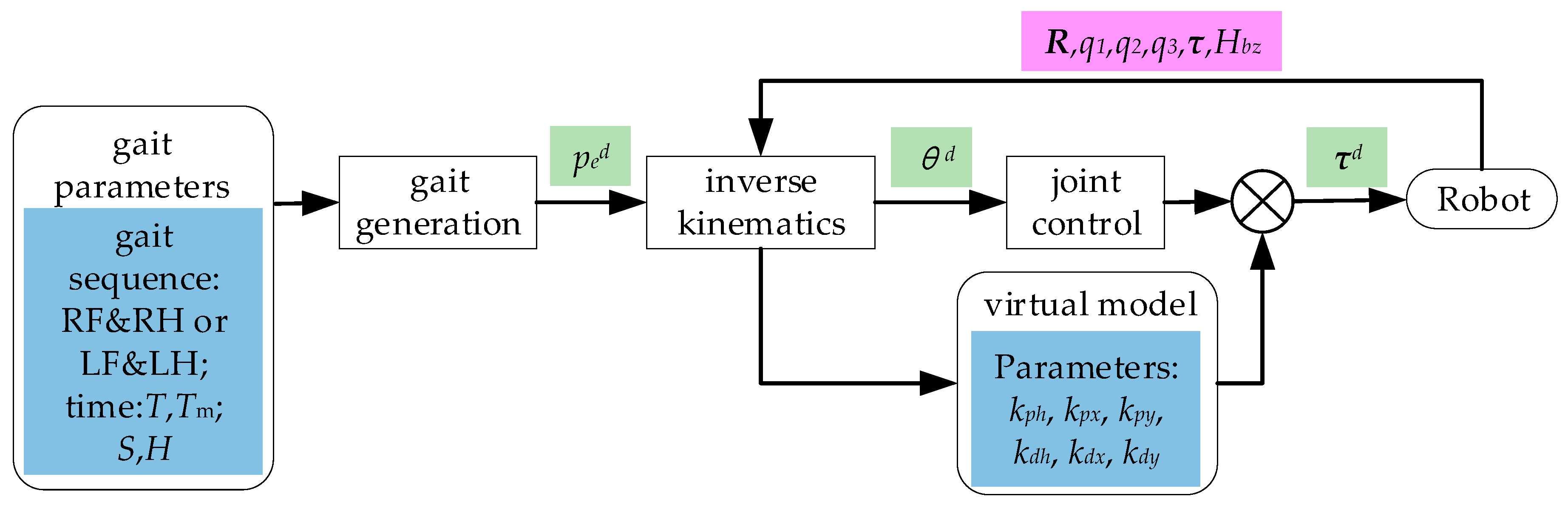
4. The Control Algorithm for a Hydraulic Quadruped Robot

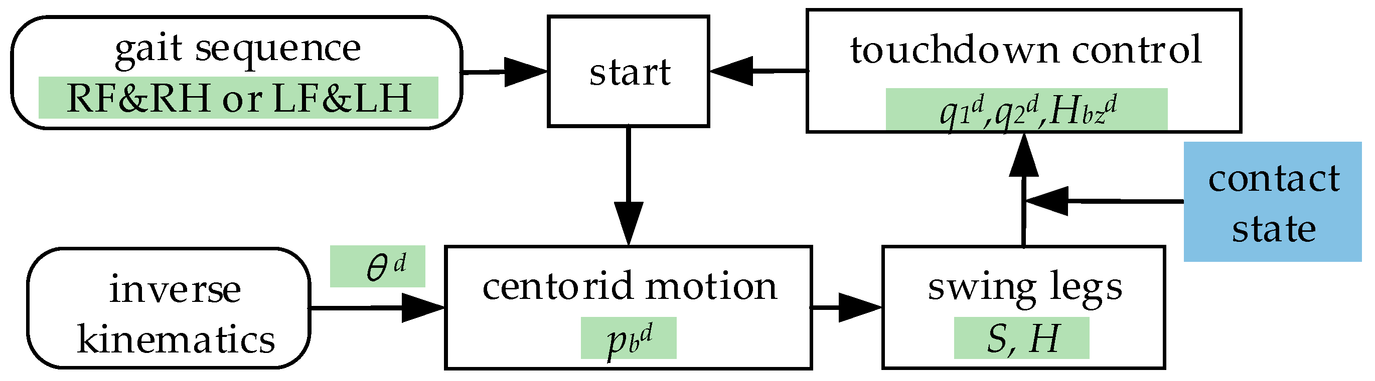
4.1. Centroid Control in Touchdown Stage

Under the ideal conditions, while the robot moves in a pacing gait, the pitch angle and yaw angle of the trunk are zero, and the attitude angles can be measured by the IMU in real time.

The control of hydraulic quadruped robots is easier when they are equipped with a set of virtual elements: a spring and damping. Those virtual actuators allow us to ignore the non-linearity due to the legs [41,42]. Three sets of virtual elements can control the rolling angle, pitching angle and height of the trunk, respectively.

For the sake of simplicity, we ignore the inertial force of the legs, hence the relationship between joint torque and generalized force acting on the trunk can be expressed as:

$$\mathit{\tau }=-{\mathit{J}}^T\mathit{F}$$

(20)

where τ = [τ₁ τ₂ τ₃]^T is the vector of joint output torque. τ₁, τ₂ and τ₃ represent rolling hip joint torque, pitching hip joint torque and pitching knee joint torque, respectively. F = [F_x F_y F_z]^T is the vector of generalized force. F_x, F_y and F_z represent the virtual force of the landing leg acting on the robot trunk along x, y and z axes.

According to the force analysis, the mapping of the moment of the landing leg acting on the robot trunk T = [T_x T_y T_z]^T to the joint torque is as follows:

$$\left[\begin{array}{c}{T}_x\\ T_y\\ T_z\end{array}\right]=\left[\begin{array}{ccc}-1& 0& 0\\ 0& -c_1& -c_1\\ 0& s_1& s_1\end{array}\right]\left[\begin{array}{c}{\tau }_1\\ {\tau }_2\\ {\tau }_3\end{array}\right]$$

(21)

Combining Equations (11), (20) and (21), we get a set of simplified equations:

$$\mathit{F}\mathit{T}=\left[\begin{array}{c}\mathit{F}\\ \mathit{T}\end{array}\right]=\left[\begin{array}{c}{F}_x\\ F_y\\ F_z\\ T_x\\ T_y\\ T_z\end{array}\right]=\left[\begin{array}{ccc}0& -s_{23}/(l_2{s}_3)& (l_2{s}_2+l_3{s}_{23})/(l_2{l}_3{s}_3)\\ -c_1/(l_1+l_2{c}_2+l_3{c}_{23})& -s_1{c}_{23}/(l_2{s}_3)& s_1(l_2{c}_2+l_3{c}_{23})/(l_2{l}_3{s}_3)\\ -s_1/(l_1+l_2{c}_2+l_3{c}_{23})& c_1{c}_{23}/(l_2{s}_3)& -c_1(l_2{c}_2+l_3{c}_{23})/(l_2{l}_3{s}_3)\\ -1& 0& 0\\ 0& -c_1& -c_1\\ 0& s_1& s_1\end{array}\right]\left[\begin{array}{c}{\tau }_1\\ {\tau }_2\\ {\tau }_3\end{array}\right]$$

(22)

Let

$${\mathit{J}}_{FT}=\left[\begin{array}{ccc}0& -s_{23}/(l_2{s}_3)& (l_2{s}_2+l_3{s}_{23})/(l_2{l}_3{s}_3)\\ -c_1/(l_1+l_2{c}_2+l_3{c}_{23})& -s_1{c}_{23}/(l_2{s}_3)& s_1(l_2{c}_2+l_3{c}_{23})/(l_2{l}_3{s}_3)\\ -s_1/(l_1+l_2{c}_2+l_3{c}_{23})& c_1{c}_{23}/(l_2{s}_3)& -c_1(l_2{c}_2+l_3{c}_{23})/(l_2{l}_3{s}_3)\\ -1& 0& 0\\ 0& -c_1& -c_1\\ 0& s_1& s_1\end{array}\right]$$

(23)

The virtual force and moment of two landing legs acting on the robot trunk can be expressed as:

$$\mathit{F}{\mathit{T}}_{FH}=\left[\begin{array}{c}\mathit{F}{\mathit{T}}_F\\ \mathit{F}{\mathit{T}}_H\end{array}\right]=\left[\begin{array}{c}{\mathit{F}}_F\\ {\mathit{T}}_F\\ {\mathit{F}}_H\\ {\mathit{T}}_H\end{array}\right]=\left[\begin{array}{cc}{\mathit{J}}_{F{T}_F}& {\mathbf{0}}_{6\times 3}\\ {\mathbf{0}}_{6\times 3}& {\mathit{J}}_{F{T}_H}\end{array}\right]\left[\begin{array}{c}{\mathit{\tau }}_F\\ {\mathit{\tau }}_H\end{array}\right]$$

(24)

where FT_FH = [F_Fx F_Fy F_Fz T_Fx T_Fy T_Fz F_Hx F_Hy F_Hz T_Hx T_Hy T_Hz]^T, in which, the subscript F denotes the foreleg, and the subscript H denotes the hind leg.

The vector of virtual force and moment acting on the centroid of the trunk can be obtained by the vector of generalized force and torque, hence FT_b = [F_bx F_by F_bz T_bx T_by T_bz]^T can be written as:

$$\{\begin{array}{l}{F}_{bx}=F_{Fx}+F_{Hx}\\ F_{by}=F_{Fy}+F_{Hy}\\ F_{bz}=F_{Fz}+F_{Hz}\\ T_{bx}=T_{Fx}+T_{Hx}+2b(F_{Fz}-F_{Hz})\\ T_{by}=T_{Fy}+T_{Hy}+2a(F_{Fz}-F_{Hz})\\ T_{bz}=T_{Fz}+T_{Hz}-2b(F_{Fy}-F_{Hy})+2a(F_{Fx}-F_{Hx})\end{array}$$

(25)

Let

$$\mathit{Q}=\left[\begin{array}{cccccccccccc}1& 0& 0& 0& 0& 0& 1& 0& 0& 0& 0& 0\\ 0& 1& 0& 0& 0& 0& 0& 1& 0& 0& 0& 0\\ 0& 0& 1& 0& 0& 0& 0& 0& 1& 0& 0& 0\\ 0& 0& 2b& 1& 0& 0& 0& 0& -2b& 1& 0& 0\\ 0& 0& 2a& 0& 1& 0& 0& 0& -2a& 0& 1& 0\\ 2a& 2b& 0& 0& 0& 1& -2a& -2b& 0& 0& 0& 1\end{array}\right]$$

(26)

We can substitute Q back into Equation (25) to get a set of simplified equations:

$$\mathit{F}{\mathit{T}}_b=\mathit{Q}·\mathit{F}{\mathit{T}}_{FH}$$

(27)

So that we can rearrange Equation (24) into the following intuitive form:

$$\mathit{F}{\mathit{T}}_b=\mathit{Q}·\left[\begin{array}{cc}{\mathit{J}}_{F{T}_F}& {\mathbf{0}}_{6\times 3}\\ {\mathbf{0}}_{6\times 3}& {\mathit{J}}_{F{T}_H}\end{array}\right]\left[\begin{array}{c}{\mathit{\tau }}_F\\ {\mathit{\tau }}_H\end{array}\right]$$

(28)

As shown in Figure 4, the resultant forces and moments at the centroid of the trunk are as follows:

$$\{\begin{array}{l}{F}_{bz}=k_{ph}(h-h^d)+k_{dh}\dot{h}\\ T_{bx}=k_{px}(q_1-q_1{}^d)+k_{dx}{\dot{q}}_1\\ T_{by}=k_{py}(q_2-q_2{}^d)+k_{dy}{\dot{q}}_2\end{array}$$

(29)

where k_ph, k_px and k_py are the elastic coefficients of the virtual components; k_dh, k_dx and k_dy are the damping coefficients of the virtual components; h^d is the desired height of the trunk; h is the actual height of the trunk; and q^1d and q^2d are the desired roll angle and pitch angle of the robot trunk. T_bx, T_by and T_bz represent the torque of the landing leg acting on the robot trunk along x, y and z axes.

The actual attitude angles and the height of the robot trunk are close to their theoretical values when choosing reasonable elastic coefficients and damping coefficients. By substituting Equation (29) into Equation (28), the following results can be obtained:

$$\left[\begin{array}{c}{F}_{bz}\\ T_{bx}\\ T_{by}\end{array}\right]=\left[\begin{array}{cccccccccccc}0& 0& 1& 0& 0& 0& 0& 0& 1& 0& 0& 0\\ 0& 0& 2b& 1& 0& 0& 0& 0& -2b& 1& 0& 0\\ 0& 0& 2a& 0& 1& 0& 0& 0& -2a& 0& 1& 0\end{array}\right]\left[\begin{array}{cc}{\mathit{J}}_{F{T}_F}& {\mathbf{0}}_{6\times 3}\\ {\mathbf{0}}_{6\times 3}& {\mathit{J}}_{F{T}_H}\end{array}\right]\left[\begin{array}{c}{\mathit{\tau }}_F\\ {\mathit{\tau }}_H\end{array}\right]$$

(30)

Let be

$${\mathit{S}}_{3\times 6}={\left[\begin{array}{cccccccccccc}0& 0& 1& 0& 0& 0& 0& 0& 1& 0& 0& 0\\ 0& 0& 2b& 1& 0& 0& 0& 0& -2b& 1& 0& 0\\ 0& 0& 2a& 0& 1& 0& 0& 0& -2a& 0& 1& 0\end{array}\right]}_{3\times 12}{\left[\begin{array}{cc}{\mathit{J}}_{F{T}_F}& {\mathbf{0}}_{6\times 3}\\ {\mathbf{0}}_{6\times 3}& {\mathit{J}}_{F{T}_H}\end{array}\right]}_{12\times 6}$$

(31)

However, it is impossible to solve all six joint torques of two landing legs according to Equation (29). Our solution allows for the output requirements of actuators so as to derive the joint torques. Therefore, the following equations are added:

$$\{\begin{array}{c}{\tau }_{F1}={\tau }_{H1}\\ {\tau }_{F2}={\tau }_{H2}\\ {\tau }_{F3}={\tau }_{H3}\end{array}$$

(32)

From Equations (25), and (29) to (32), the joint torques of the two landing legs can be concluded:

$$\left[\begin{array}{c}{\tau }_{F1}\\ {\tau }_{F2}\\ {\tau }_{F3}\\ {\tau }_{H1}\\ {\tau }_{H2}\\ {\tau }_{H3}\end{array}\right]={\left[\begin{array}{c}\mathit{S}\\ \mathit{P}\end{array}\right]}^{-1}\left[\begin{array}{c}{k}_{ph}(h-h^d)+k_{dh}\dot{h}\\ k_{px}(q_1-q_1{}^d)+k_{dx}{\dot{q}}_1\\ k_{py}(q_2-q_2{}^d)+k_{dy}{\dot{q}}_2\\ 0\\ 0\\ 0\end{array}\right]$$

(33)

where

$$\mathit{P}=\left[\begin{array}{cccccc}1& 0& 0& -1& 0& 0\\ 0& 1& 0& 0& -1& 0\\ 0& 0& 1& 0& 0& -1\end{array}\right]$$

(34)

As shown in Equation (33), the roll angle, pitch angle and height of the trunk can be controlled with reference to the joint torques of the landing leg of the hydraulic quadruped robot.

4.2. The Design of a Centroid-Based Controller

Figure 5 presents the block of the centroid-based controller for the hydraulic quadruped robot. The superscript d in ensuing figures represents the expected value of each variable. Light green blocks indicate user-defined parameters. Light blue blocks indicate control parameters, while light pink blocks indicate feedback parameters. The trajectory of the robot, generated by the gait parameters given and the motion of the swing leg, is controlled. After the robot leg touches the ground, the position and attitude of the trunk are controlled by virtual model. Moreover, the input parameters are adjusted in real time by using the feedback information of sensors which are fixed on the robot.

The block diagram of a centroid-based controller for the hydraulic quadruped robot depicted in Figure 6. We assume that the hydraulic quadruped robot starts with all four legs touching the ground. On the basis of kinematic derivations, the centroid trajectory of the trunk is planned, while the state machine controls a pair of legs as swinging legs according to the specified gait sequence. Once the change of contact state is detected, the control state will be switched. The change of contact state is determined by control algorithm or sensor feedback. Then the current legs are controlled in the touchdown phase and the other pair legs are controlled in the swing phase.

5. Simulation and Analysis

5.1. Simulation Environment

In order to verify the effectiveness of the proposed method, the dynamic simulations were carried out in dynamic simulation software ADAMS. The virtual prototype model in the simulation had the same size and mass distribution as the HD platform developed by the Hydraulic Quadruped Robot Joint Lab of Harbin University of Science and Technology. The parameters of the simulation model are shown in

Table 1. Simulation parameters of hydraulic quadruped robot.

Parameters	Values
cycle time	0.8 s
stride length	200 mm
max foot height	50 mm
simulation time	8 s
gravity acceleration	9.8 m/s2
static friction coefficient	0.6
dynamic friction coefficient	0.2

.

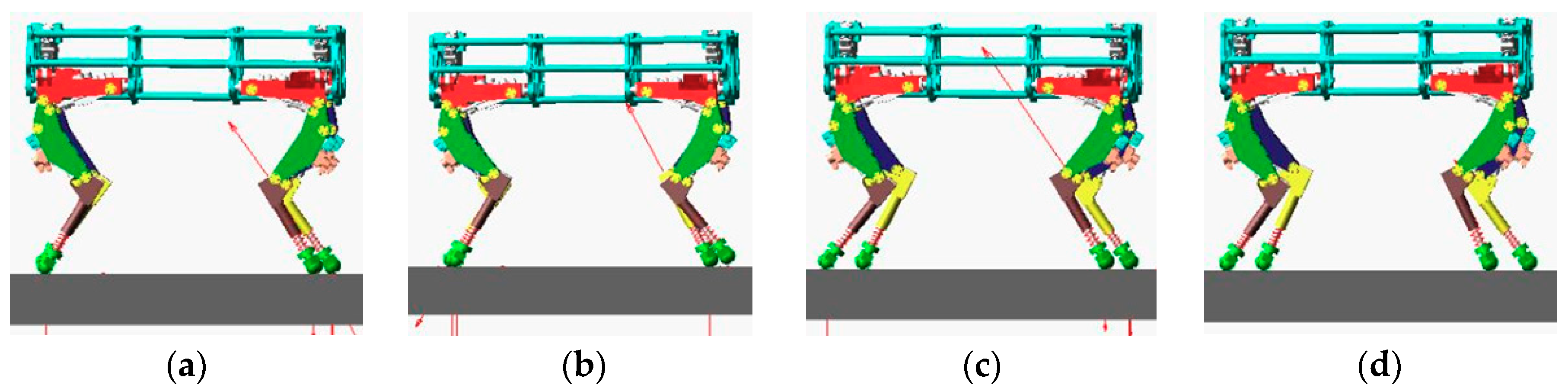
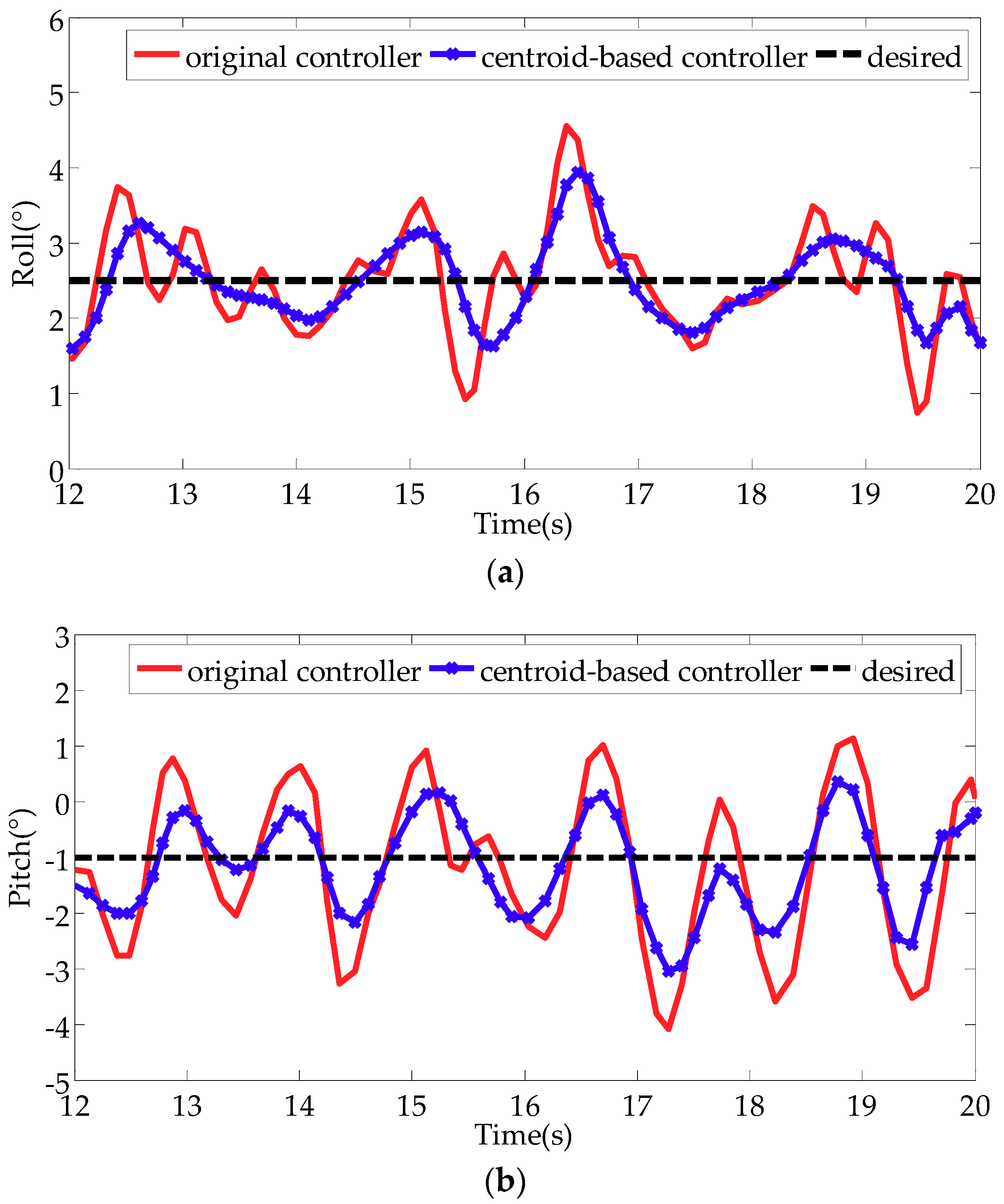
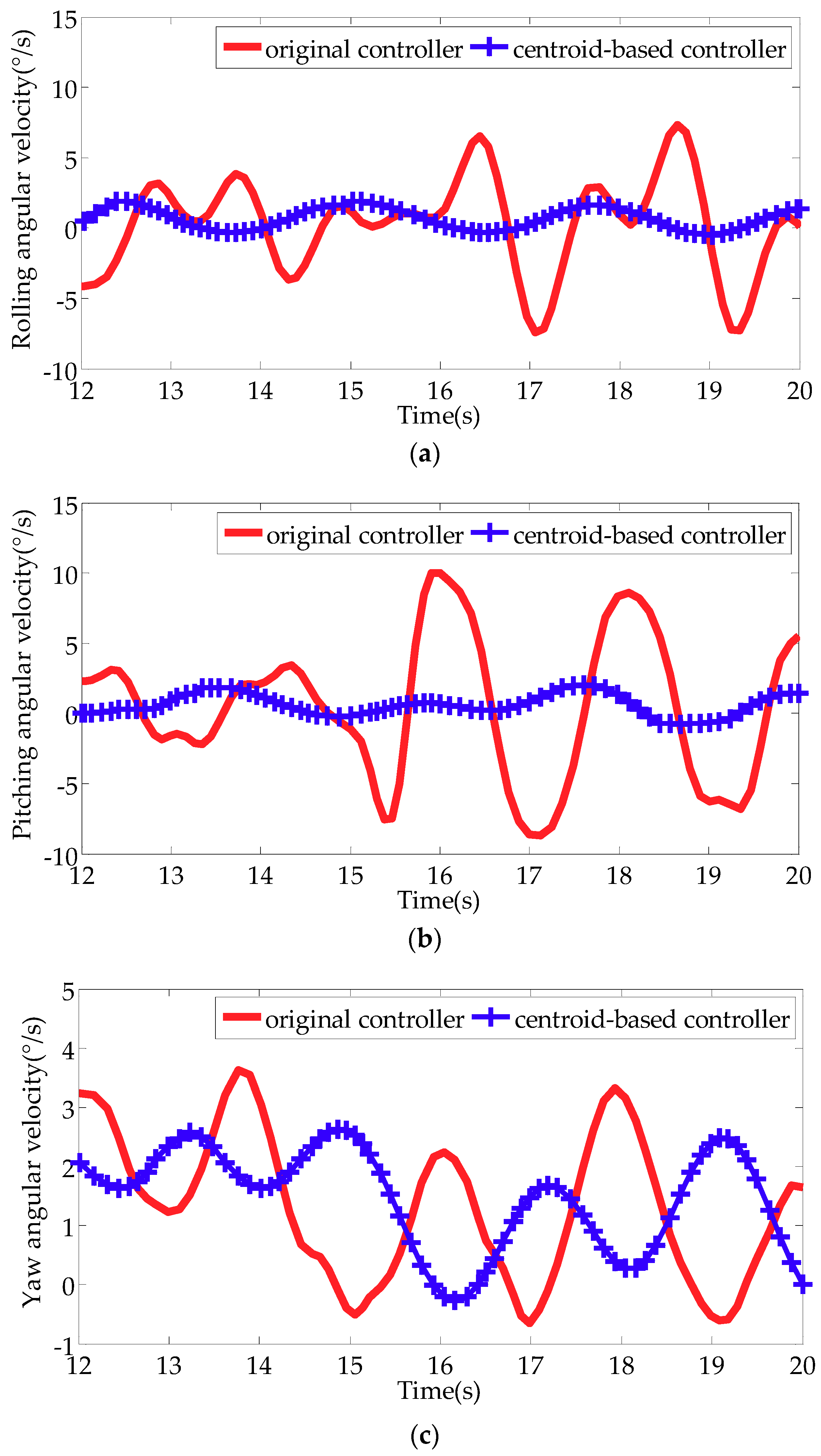
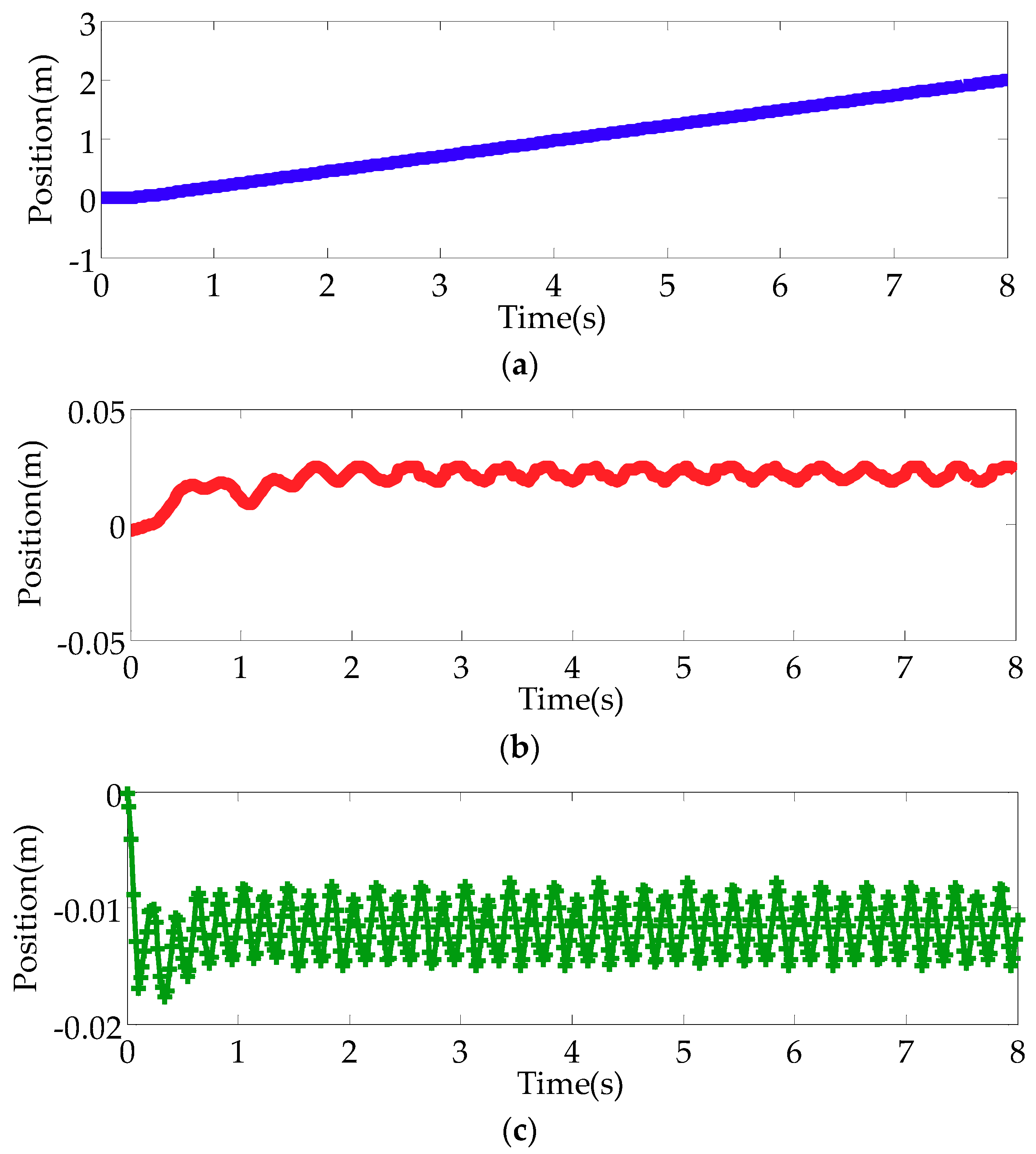
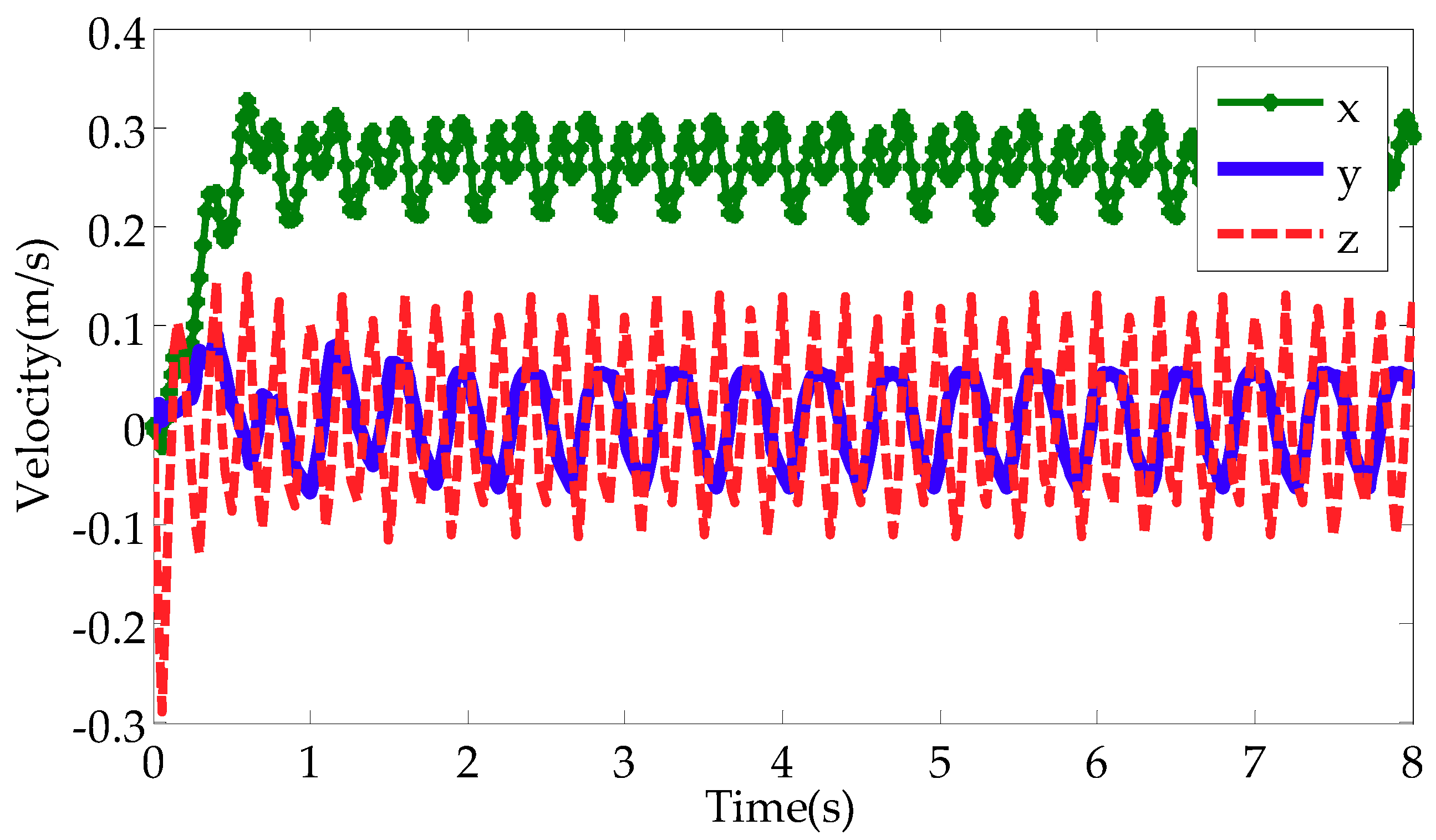
5.2. Simulation Results and Analysis

In a cycle, two pairs of legs alternately swing and support. In the initial stage, the robot is supported by four legs. Next, RF and RH legs are in the swing stage. Then, RF and RH legs are in the supporting stage. The motion process of the quadruped robot is shown in Figure 7.

To measure the motion of the hydraulic quadruped robot, the displacement curves of the centroid of the robot trunk are shown in Figure 8. Figure 8a–c shows displacement curves along x, y and z-axes, respectively. It can be concluded that the motion of the robot tends to be stable after two cycles of acceleration. When the RF leg and the RH leg are raised, it marks the beginning of the motion cycle. At the beginning of the cycle, the centroid of the trunk has a small displacement in the opposite direction of the forward direction. Figure 8a shows the forward displacement of the hydraulic quadruped robot is two meters in ten motion cycles. Figure 8b shows that the robot has generated laterality motion during pacing gait. The main reason is that the center of gravity of the trunk moved to the same side when the one pair legs of the robot first touched the ground. When the other side legs touched the ground, the center of gravity of the trunk moved to the other side. As shown in Figure 8c, the centroid of the robot trunk varies from −16 mm to −10 mm in the vertical direction. In order to reduce the impact force of the ground, a shock absorber spring is added to the shank of the robot in the design of the mechanical structure. The fluctuation of the hydraulic quadruped robot trunk is small in the vertical direction by the proposed control method, which verifies the effectiveness of the proposed height control strategy.

The velocity curves of the centroid of the robot trunk are shown in Figure 9. As seen from Figure 9, the speed of the robot in the forward direction is stable at about 0.25 m/s. The lateral velocity range of the robot trunk varies from −0.1 m/s to 0.1 m/s, and changes symmetrically along the y-axis. The sudden change of velocity in the vertical direction is caused by the impact of the ground on the robot when the foot touches the ground.

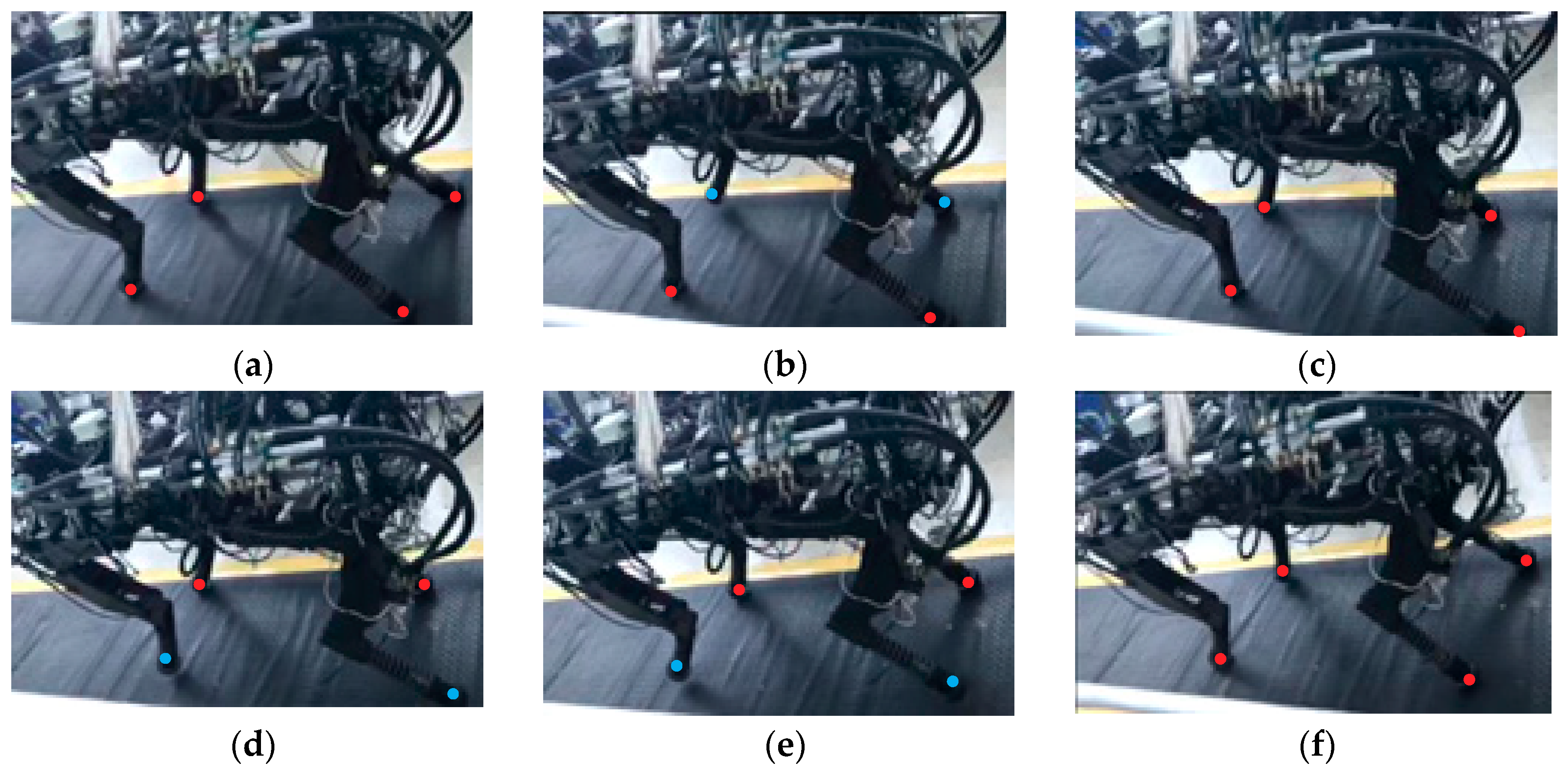
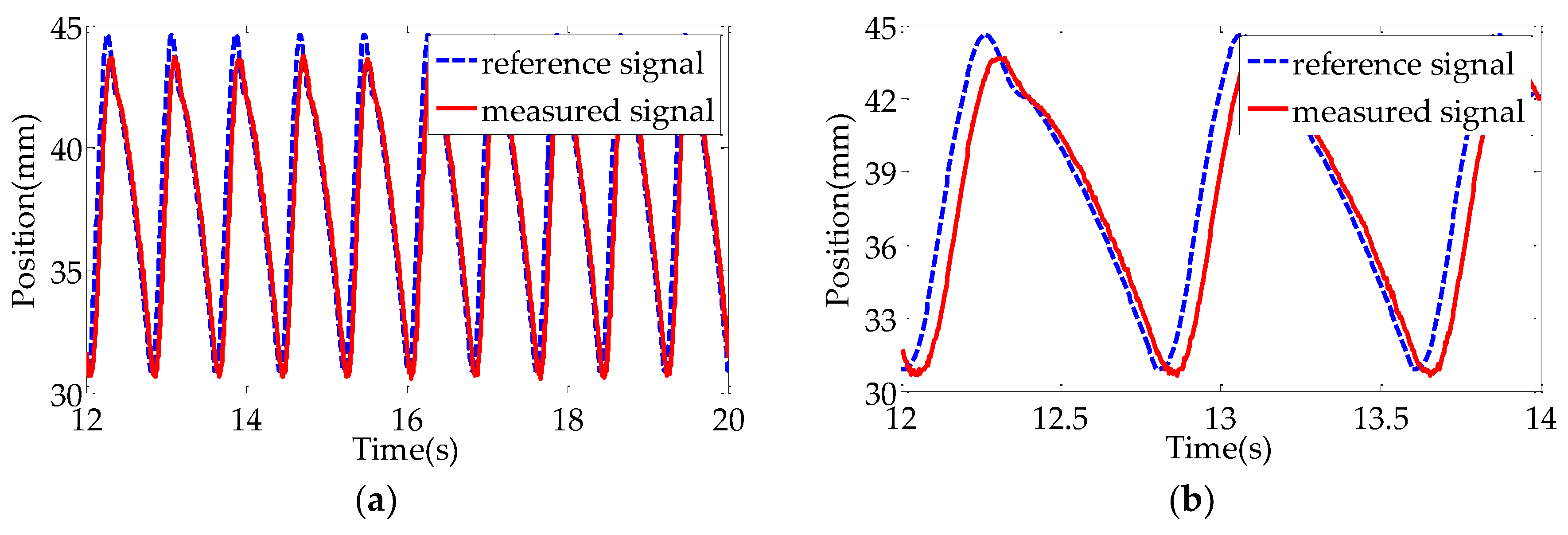
6. Experimental Analysis

To certify the effectiveness of the proposed control strategy in practical robots, the designed controller was applied to a hydraulic quadruped robot developed by the Hydraulic Quadruped Robot Joint Lab of Harbin University of Science and Technology.

The experimental platform of the hydraulic quadruped robot is illustrated in Figure 10. The electro-hydraulic servo valve was the SFL212F-12/8-21-40 two-stage force feedback asymmetric servo valve, produced by the 18th Research Institute of the First Academy of China Aerospace Science and Technology Corporation (Beijing, China). The displacement sensor was the LVDT-PA1HL60X sensor produced by Fuxin Lisheng Automatic Control Co., Ltd. (Fuxin, China). The force sensor was the WMC-3000 Sensor produced by the Interface Company of America (Phenix City, AL, USA). The IMU was the XW-G15615 produced by Starneto (Beijing, China).

In the experiment, the duty cycle of the robot pace gait was 0.5; that is, the swing phase and the support phase were equal in time. The period time was 0.8s, the stride length was 200 mm, and the maximum height of the foot was 50 mm. The experimental process of pace gait motion of the hydraulic quadruped robot is shown in Figure 11. In the picture, the red solid point represents the supporting leg, and the blue one represents the swinging leg. During a motion cycle, a pair of legs of the hydraulic quadruped robot went through lifting, falling and supporting stages.

The variations of attitude angle and attitude angular velocity of the robot trunk detected by IMU are shown in Figure 12 and Figure 13, respectively. The curves of original controller represent the experimental data obtained without the proposed controller. It only planned the foot trajectory based on the kinematic analysis of the single leg of the quadruped robot, but did not plan and control the centroid of the robot trunk. The curve of centroid-based controller represents the experimental data obtained with the proposed controller. The proposed controller includes foot trajectory planning, and the trajectory planning of the trunk centroid and centroid control of the trunk. During the motion of the hydraulic quadruped robot in pacing gait, since the right leg and the left leg alternately lie in the supporting phase and swing phase, the robot trunk alternately leans to either side. The attitude angles of the robot trunk change slightly in Figure 12. In ten period cycles, when the proposed controller was not used, the roll angle of the hydraulic quadruped robot ranged from 0.6 to 4.5 degrees, and the pitch angle ranged from −4.2 to 1.13 degrees. When using the presented control method, the roll angle ranged from 1.58 to 3.94 degrees, and the pitch angle ranged from −3 to 0.35 degrees.

From Figure 13, it can be seen that the attitude angular velocity of the trunk of the hydraulic quadruped robot changed smoothly, by the proposed controller. The results show that the fluctuation of the robot trunk is small during the movement of the robot. As seen from the experimental process, the motion of each leg of the robot is coordinated, and the robot can move smoothly and straight. The availability and rationality of the proposed control method are further proved.

The position tracking curves of the electro-hydraulic servo actuator of the robot in pacing gait are illustrated in Figure 14 and Figure 15. The reference signals were obtained by cycloid trajectory planning. The measured signals are the positional variations of the piston rods of the robot’s actuators detected by the displacement sensors attached to the actuators. As can be seen from the figures, the whole tracking process is compact. The effectiveness of the proposed control method based on centroid trajectory is further verified.

7. Conclusions

In order to enhance the stability of hydraulic quadruped robots in motion, this paper presents a centroid-based controller for quadrupedal pacing. The centroid control of the hydraulic quadruped robot trunk was added to the control of the whole robot. The kinematic model of the whole hydraulic quadruped robot was established, and the relationship between each leg and the robot trunk was described. The coupling of trunk motion and leg motion was explained in detail. The real-time attitude feedback information of the trunk centroid was introduced into the trajectory planning of the trunk centroid. Joint torques that fulfilled the minimization of the contact forces were calculated. The positions and attitudes of the robot trunk were adjusted by the spring damper virtual elements. The performance of the proposed framework was tested in simulation and on a robot platform. The motion attitude data of hydraulic quadruped robot with or without the proposed controller were compared. The experimental results showed that the robot trunk moved more smoothly with the proposed controller than that without the proposed controller. The stable and accurate dynamic motion was accomplished, which verified the effectiveness and feasibility of the proposed control strategy. The centroid-based controller can be extended to the other dynamic gaits of quadruped robots, as long as the corresponding parameters and models are changed. In the near future, our work is to study the stability of robots in complex working environments.

References

1. Li, X.; Gao, H.; Zha, F.; Li, J.; Wang, Y.; Guo, Y.; Wang, X. Learning the cost function for foothold selection in a quadruped robot. Sensors 2019, 19, 1292. [Google Scholar] [CrossRef] [PubMed]
2. Yang, K.; Li, Y.; Zhou, L.; Rong, X. Energy efficient foot trajectory of trot motion for hydraulic quadruped robot. Energies. 2019, 12, 2514. [Google Scholar] [CrossRef]
3. Mattila, J.; Koivumaki, J.; Caldwell, D.-G.; Semini, C. A survey on control of hydraulic robotic manipulators with projection to future trends. IEEE-ASME Trans. Mechatron. 2017, 22, 669–680. [Google Scholar] [CrossRef]
4. Ba, K.; Yu, B.; Gao, Z.; Li, W.; Ma, G.; Kong, X. Parameters sensitivity analysis of position-based impedance control for bionic legged robots’ HDU. Appl. Sci. 2017, 7, 1035. [Google Scholar] [CrossRef]
5. Raibert, M.; Blankespoor, K.; Nelson, G.; Playter, R. BigDog, the rough-terrain quadruped robot. IFAC Proc. Vol. 2008, 41, 10822–10825. [Google Scholar] [CrossRef]
6. Yang, K.; Rong, X.; Zhou, L.; Li, Y. Modeling and analysis on energy consumption of hydraulic quadruped robot for optimal trot motion control. Appl. Sci. 2019, 9, 1771. [Google Scholar] [CrossRef]
7. Focchi, M.; Del Prete, A.; Havoutis, I.; Featherstone, R.; Caldwell, D.-G.; Semini, C. High-slope terrain locomotion for torque-controlled quadruped robots. Auton. Robot. 2017, 41, 259–272. [Google Scholar] [CrossRef]
8. Park, H.-W.; Kim, S. Quadrupedal galloping control for a wide range of speed via vertical impulse scaling. Bioinspir. Biomim. 2015, 10, 025003. [Google Scholar] [CrossRef] [PubMed]
9. Wayne, P. Alpha dogs: how political spin became a global business. Int. Aff. 2009, 85, 168–169. [Google Scholar]
10. Wensing, P.-M.; Wang, A.; Seok, S.; Otten, D.-M.; Lang, J.-H.; Kin, S. Proprioceptive actuator design in the MIT Cheetah: impact mitigation and high-bandwidth physical interaction for dynamic legged robots. IEEE Trans. Robot. 2017, 99, 1–14. [Google Scholar] [CrossRef]
11. Dynamics, B. Spot Classic: Takes a Kicking and Keeps on Ticking. Available online: https://www.bostondynamics.com/spot-classic (accessed on 11 July 2019).
12. Dynamics, B. Spot: Good Things Come in Small Packages. Available online: https://www.bostondynamics.com/spot (accessed on 11 July 2019).
13. Hutter, M.; Gehring, C.; Lauber, A.; Gunther, F.; Bellicoso, C.-D.; Tsounis, V.; Fankhauser, P.; Diethelm, R.; Bachmann, S.; Bloesch, M.; et al. ANYmal - toward legged robots for harsh environments. Adv. Robot. 2017, 31, 1–14. [Google Scholar] [CrossRef]
14. Semini, C.; Tsagarakis, N.-G.; Guglielmino, E.; Focchi, M.; Cannella, F.; Caldwell, D.-G. Design of HyQ—A hydraulically and electrically actuated quadruped robot. Proc. Inst. Mech. Eng. Part I-J. Syst. Control Eng. 2011, 225, 831–849. [Google Scholar] [CrossRef]
15. Khan, H.; Kitano, S.; Frigerio, M.; Camurri, M.; Barasuol, V.; Featherstone, R.; Caldwell, D.-G.; Semini, C. Development of the lightweight hydraulic quadruped robot –MiniHyQ. In Proceedings of the 2015 IEEE International Conference on Technologies for Practical Robot Applications (TePRA), Woburn, MA, USA, 11–12 May 2013. [Google Scholar]
16. Semini, C.; Barasuol, V.; Goldsmith, J.; Frigerio, M.; Focchi, M.; Gao, Y.; Caldwell, D.-G. Design of the hydraulically-actuated, torque-controlled quadruped robot HyQ2Max. IEEE-ASME Trans. Mechatron. 2016, 99, 1–12. [Google Scholar] [CrossRef]
17. Rong, X.; Li, Y.; Ruan, J.; Li, B. Design and simulation for a hydraulic actuated quadruped robot. J. Mech. Sci. Technol. 2012, 26, 1171–1177. [Google Scholar] [CrossRef]
18. Chen, T.; Rong, X.; Li, Y.; Ding, C.; Chai, H.; Zhou, L. A compliant control method for robust trot motion of hydraulic actuated quadruped robot. Int. J. Adv. Robot. Syst. 2018, 15, 1–16. [Google Scholar] [CrossRef]
19. Hudson, P.-E.; Corr, S.-A.; Wilson, A.-M. High speed galloping in the cheetah (Acinonyx jubatus) and the racing greyhound (Canis familiaris): spatio-temporal and kinetic characteristics. J. Exp. Biol. 2012, 215, 2425–2434. [Google Scholar] [CrossRef] [PubMed]
20. Moro, F.-L.; Sprowitz, A.; Tuleu, A.; Vespignani, M.; Tsagarakis, N.-G.; Ijspeert, A.-J.; Caldwell, D.-G. Horse-like walking, trotting, and galloping derived from kinematic motion primitives (kMPs) and their application to walk/trot transitions in a compliant quadruped robot. Biol. Cybern. 2013, 107, 309–320. [Google Scholar] [CrossRef] [PubMed]
21. Chung, J.-W.; Lee, I.-H.; Cho, B.-K.; Oh, J.-H. Posture stabilization strategy for a trotting point-foot quadruped robot. J. Intell. Robot. Syst. 2013, 72, 325–341. [Google Scholar] [CrossRef]
22. Havoutis, I.; Semini, C.; Buchli, J.; Caldwell, D.-G. Quadrupedal trotting with active compliance. In Proceedings of the 2013 IEEE International Conference on Mechatronics, Vicenza, Italy, 27 February–1 March 2013; pp. 604–609. [Google Scholar]
23. Cai, R.; Chen, Y.; Hou, W.; Wang, J.; Ma, H. Trotting gait of a quadruped robot based on the time-pose control method. Int. J. Adv. Robot. Syst. 2013, 10, 108. [Google Scholar]
24. Gehring, C.; Coros, S.; Hutter, M.; Bloesch, M.; Hoepflinger, M.-A.; Siegwart, R. Control of dynamic gaits for a quadrupedal robot. In Proceedings of the IEEE International Conference on Robotics and Automation, Karlsruhe, Germany, 6–10 May 2013; pp. 3287–3292. [Google Scholar]
25. He, D.; Ma, P.; Cao, X.; Cao, C.; Yu, H. Impact of initial stance of quadruped trotting on walking stability. Robot 2004, 26, 529–532+537. [Google Scholar]
26. Xie, H.; Shang, J.; Luo, Z.; Xue, Y. Body rolling analysis and attitude control of a quadruped robot during trotting. Robot 2014, 36, 676–682. [Google Scholar]
27. Hayat, A.-A.; Elangovan, K.; Elara, M.-R.; Teja, M.-S. Tarantula: Design, Modeling, and Kinematic Identification of a Quadruped Wheeled Robot. Appl. Sci. 2019, 9, 94. [Google Scholar] [CrossRef]
28. Boussema, C.; Powell, M.-J.; Bledt, G.; Ijspeert, A.-J.; Wensing, P.-M.; Kim, S. Online gait transitions and disturbance recovery for legged robots via the feasible impulse set. IEEE Robot. Auto. Letters 2019, 4, 1611–1618. [Google Scholar] [CrossRef]
29. Tran, D.-T.; Koo, I.-M.; Lee, Y.-H.; Moon, H.; Koo, J.; Park, S.; Choi, H.-R. Motion control of a quadruped robot in unknown rough terrain using 3D spring damper leg model. Int. J. Control Autom. Syst. 2014, 12, 372–382. [Google Scholar] [CrossRef]
30. Fukui, T.; Fujisawa, H.; Otaka, K.; Fukuoka, Y. Autonomous gait transition and galloping over unperceived obstacles of a quadruped robot with CPG modulated by vestibular feedback. Robot. Auton. Syst. 2018. [Google Scholar] [CrossRef]
31. Park, H.-W.; Ramezani, A.; Grizzle, J.-W. A finite-state machine for accommodating unexpected large ground-height variations in bipedal robot walking. IEEE Trans. Robot. 2013, 29, 331–345. [Google Scholar] [CrossRef]
32. Bhattacharya, A.; Bijan, S.; Mukherjee, S.-K. Integrating AHP with QFD for robot selection under requirement perspective. Int. J. Prod. Res. 2005, 43, 3671–3685. [Google Scholar] [CrossRef]
33. Chai, H.; Meng, J.; Rong, X.; Li, Y. Design and implementation of SCalf, an advanced hydraulic quadruped robot. Robot 2014, 36, 385–391. [Google Scholar]
34. Sakakibara, Y.; Kan, K.; Hosoda, Y.; Hattori, M.; Fujie, M. Foot trajectory for a quadruped walking machine. Proceedings of IEEE International Workshop on Intelligent Robots and Systems, Ibaraki, Japan, 3–6 July 1990; pp. 315–322. [Google Scholar]
35. Li, B.; Li, Y.; Rong, X.; Meng, J. Trotting gait planning and implementation for a little quadruped robot. In Proceedings of the 2011 International Conference on Electric and Electronics, Nanchang, China, 20–22 June 2011; pp. 195–202. [Google Scholar]
36. Li, Y.; Li, B.; Rong, X.; Meng, J. Mechanical design and gait planning of a hydraulically actuated quadruped bionic robot. J. Shandong Univ. Eng. Sci. 2011, 41, 32–36. [Google Scholar]
37. Zhang, S.; Rong, X.; Li, Y.; Li, B. Static gait planning method for quadruped robots on rough terrains. J. Jilin Univ. (Eng. Technol. Ed.) 2016, 46, 1287–1296. [Google Scholar]
38. Lei, J.; Jia, G. Control of quadruped robot with trot gait. J. Shanghai Univ. (Nat. Sci.) 2017, 23, 882–892. [Google Scholar]
39. Kim, K.-Y.; Park, J.-H. Ellipse-based leg-trajectory generation for galloping quadruped robots. J. Mech. Sci. Technol. 2008, 22, 2099–2106. [Google Scholar] [CrossRef]
40. Wang, L.; Wang, J.; Wang, S.; He, Y. Strategy of foot trajectory generation for hydraulic quadruped robots gait planning. Chin. J. Mech. Eng. 2013, 49, 39–44. [Google Scholar] [CrossRef]
41. Pratt, J.; Torres, A.; Dilworth, P.; Pratt, G. Virtual actuator control. In Proceedings of the 1996 IEEE/RSJ International Conference on Intelligent Robots and Systems, Osaka, Japan, 4–8 November 1996; pp. 1219–1226. [Google Scholar]
42. Pratt, J.; Chew, C.-M.; Torres, A.; Dilworth, P.; Pratt, G. Virtual model control: An intuitive approach for bipedal locomotion. Int. J. Robot. Res. 2001, 20, 129–143. [Google Scholar] [CrossRef]
Figure 1. Model of hydraulic quadruped robot.
Applsci 09 03911 g001
Figure 2. Kinematics model of hydraulic quadruped robot.
Applsci 09 03911 g002
Figure 3. Height model of the robot supported by two feet.
Applsci 09 03911 g003
Figure 4. Centroid control model of hydraulic quadruped robot.
Applsci 09 03911 g004
Figure 5. Block diagram of controller frame.
Applsci 09 03911 g005
Figure 6. Schematic diagram of the state machine used in the control algorithm.
Applsci 09 03911 g006
Figure 7. Snapshots of the robot pacing on the flat ground. (a) Initial stage. (b) The right foreleg (RF) and the right hindleg (RH) are in the swing stage. (c) The left foreleg (LF) and left hindleg (LH) are in the swing stage. (d) Four legs are in the supporting stage.
Applsci 09 03911 g007
Figure 8. Displacement curves for centroid of robot trunk. (a) Position variations along x-axis. (b) Position variations along y-axis. (c) Position variations along z-axis.
Applsci 09 03911 g008
Figure 9. Velocity curves for the centroid of the robot trunk.
Applsci 09 03911 g009
Figure 10. The test platform of hydraulic quadruped robot.
Applsci 09 03911 g010
Figure 11. The pacing gait motion of the hydraulic quadruped robot in a gait period. (a) Initial stage. (b) RF and RH leg are in the support stage. (c) All legs are in the supporting stage. (d) RF and RH leg are in the lifting stage. (e) RF and RH legs are at their highest points. (f) Touch down stage.
Applsci 09 03911 g011
Figure 12. Attitude angle curves of the robot trunk. (a) Roll angle of the robot trunk. (b) Pitch angle of the robot trunk.
Applsci 09 03911 g012
Figure 13. Angular velocity curves of robot trunk. (a) Rolling angle. (b) Pitching angle. (c) Yaw angle.
Applsci 09 03911 g013
Figure 14. The pitching hip joint position tracking curves of the RF leg of the robot. (a) Response curves; (b) Local amplification curves.
Applsci 09 03911 g014
Figure 15. The pitching knee joint position tracking curves of RF leg of the robot. (a) Response curves; (b) Local amplification curves.
Applsci 09 03911 g015