Anti-Slip Gait Planning for a Humanoid Robot in Fast Walking

Abstract

Humanoid robots are expected to have broad applications due to their biped mobility and human-like shape. To increase the walking speed, it is necessary to increase the power for driving the joints of legs. However, the resulting mass increasing of the legs leads to a rotational slip when a robot is walking fast. In this paper, a 3D three-mass model is proposed, in which both the trunk and thighs are regarded as an inverted pendulum, and the shanks and feet are considered as mass-points under no constraints with the trunk. Then based on the model, a friction constraint method is proposed to plan the trajectory of the swing leg in order to achieve the fastest walking speed without any rotational slip. Furthermore, the compensation for zero-moment point (ZMP) is calculated based on the 3D three-mass model, and the hip trajectory is obtained based on the compensated ZMP trajectory by using the preview control method, thus improving the robot’s overall ZMP follow-up effect. This planning method involves simple calculations but reliable results. Finally, simulations confirm that the rotational slip is avoided while stable and fast walking is realized, with free joints of the waist and arms, which then could be planned for other tasks.

1. Introduction

Humanoid robots can enter non-structural environments that wheeled and crawler robots find difficulties to reach or pass through by virtue of their biped mobility advantages [1,2,3]. Their flexible hands and arms can use human tools. Furthermore, the human-like shape helps them to assimilate into human society. Therefore, humanoid robots are expected to have broad applications in rescue and relief, public service and family service, etc. Since the release of P2 by Honda in the late 1990s, research on humanoid robots has been a major area of interest, and significant progress has been made in mechanical structures, electrical systems, and control algorithms [4,5,6,7]. However, there have been many weaknesses and problems in humanoid robots so far, e.g., low walking speed, tipping over easily, and an inability to perform other tasks while walking. In the DAPPA Robotics Challenge (DRC), humanoid robots of several teams fell down while they were on the move or performing their duties. The first-ranked DRC-HUBO completed multiple tasks relying on the wheels mounted on the knees [8]. Therefore, in order to become practical, humanoid robots must achieve stable and fast walking, and have the ability to complete other tasks while traveling.

From the point of view of hardware, in order to achieve fast walking, it is necessary to increase the driving power of each joint of the legs. There are two options for implementation. One is to use a hydraulic drive which is similar to that used in the Boston Dynamics’ Atlas robot [9]. In this option, since the power is transmitted from the body to the end actuator through the hydraulic line, the light weight of the leg is ensured [10]. However, the hydraulic system has shortcomings such as liquid leakage, high noise and a complicated system, so its further development is not optimistic. The other option is to use high-power motors or multiple motors in parallel. This configuration is easier with little noise, which is then employed in many laboratories. Figure 1 shows a typical motor-driven humanoid robot model. The robot has 6 degrees of freedom for each leg and a six-dimensional force-torque (F-T) sensor for each ankle. In addition, there is always an inertial measurement unit (IMU) fixed inside the chest. P2, HRP-5P, BHR-5, et al. have the similar leg configuration and sensors [4,5,6]. In this type of structure, since the motor must be placed inside or near its corresponding joint, and the harmonic drive gear associated with it is also heavy, the weight of the leg is greatly increased. When the robot is walking fast, the swing leg creates a large yaw moment on the support leg. When a moment generated by the friction between the ground and the sole is insufficient to offset this yaw moment, rotational slip occurs to the robot. Rotational slip is very harmful, specifically, it will make the robot deviate from a predetermined travel route and motion state, causing the robot to become unstable or even tip over. Therefore, it is necessary to overcome the rotational slip by using motion planning or a control algorithm to improve the stability of fast walking.

Traditional methods are to compensate for the yaw moment by planning motions of some joints. According to the recordings in current papers, rotation of the waist in the yaw direction is utilized to compensate the moment in some cases [11,12], or swinging of the arms is used to generate the reverse torque [13,14], or both of these two are employed at the same time [15,16]. Each method above could have certain effects, but joints of waists or arms that are used in these systems for moment compensation can’t be planned for other tasks, which weakens the ability to multi-task while walking. To address these problems, R. Cisneros et al. proposed an on-line compensation scheme for the yaw moment, which allows using the motion of every single link of the robot to contribute to the compensation, and achieved good results in the simulation of the kicking action [17,18]. However, this method could only be used for force-controlled robots, and there is no simulation or experiment applied to the robots’ walking. Therefore, none of the above methods satisfy the needs of fast-walking robots in real life. To overcome the shortcomings of these methods mentioned above, in this paper, we try to find a gait pattern with optimized yaw moment to satisfy the friction constraints. Joints of waist or arms are not used when gait planning, so they can be planned for other tasks.

In order to calculate the friction constraints and plan for the walking pattern, we need a reasonable calculation model. Multi-link model provides high precision, but it’s too complicated to use to meet the needs of real-time control. An inverted pendulum model or inverted pendulum flywheel model is simple in structure and convenient in calculation, but they can only be applied to robots with lightweight legs [11,19]. That’s because the mass of the inverted pendulum model is concentrated at one point, which is called the center of mass (CoM) and is usually mapped into the chest of the robot. The deviation of motion state between the model and the real robot grows with the growing of the leg’s mass and the deviation also grows with the increasing of the walking speed, which adds difficulties to control strategies. Therefore, in this paper, learning from the achievements of predecessors, we proposed a 3D three-mass model. In our model, we regarded both trunk and thighs as an inverted pendulum, and the shanks and feet as mass-points under no constraints with the trunk. Then we used this model to calculate the friction constraints between the ground and the sole, as well as the pattern of the swing leg conveniently with enough precision.

Hip trajectory directly affects the stability of the robot. Q. Huang et al. proposed a method to plan the hip trajectory by traversing the search with 2 key parameters [20]. However, this method requires repeated calculations to obtain a higher stability gait, which is complicated and not practical. The preview control method proposed by S. Kajita directly takes the zero-moment point (ZMP) Equation as a constraint condition, and then obtains a smooth trajectory of CoM that takes into account both the robot’s stability and the CoM’s acceleration increment by means of quadratic optimization [21]. But it relies heavily on the accuracy of modeling, so it is very effective on humanoid robot with light legs but has poor performance in robots with heavy legs. However, as described above, under the current technical conditions, an increase in leg mass due to an increasing demand in driving power is unavoidable. Therefore, in this paper, we improved the preview control method based on the 3D three-mass model. We added compensation to the reference ZMP, and finally obtained a hip trajectory that enables the robot to achieve a large stability margin.

With the trajectories of swing leg and hip, we obtained the trajectory of every joint of legs by using inverse kinematics, which means complete gait planning. Simulation experiments have shown that both the motion of the swing leg and the ZMP trajectory have an effect on the rotational slip. The gait planning method proposed in this paper can effectively avoid the robot’s rotational slip generated during fast walking. The actual ZMP follows well for the reference ZMP, thus ensuring the stability.

The rest of this paper is organized as follows: Section 2 proposes the 3D three-mass model; in Section 3, friction constraint is calculated and trajectory of the swing leg is planned; Section 4 records the planning of hip trajectory; and the simulations and conclusions are presented in Section 5 and Section 6 respectively.

2. Dynamics Model

As a ratio of a leg’s mass to the total mass of the robot increases, the effect of the legs’ motion states on the overall motion state increases. Therefore, the inverted pendulum model that treats the robot as a mass point no longer works. To this end, J. H. Park et al. proposed a gravity compensation inverted pendulum model (GCIPM), which conducts calculations after separating the swing leg’s mass from the total mass of the robot, thus increasing calculation accuracy [22]. T. Sato et al. further proposed a three-mass model for the humanoid robot, which divided the robot into a body, support leg and swing leg, and the adopted mass of these three parts to calculate the zero-moment point (ZMP) of the robot, which resulted in a smaller ZMP error and a walk mode with higher efficiency [23,24]. However, in his model, the legs’ motion states were affected by the state of the body and feet in turn, increasing the computational complexity. In fact, shanks and feet have much greater effects on the whole body’s dynamics than thighs due to their longer distances from the trunk. Therefore, we proposed a new 3D three-mass model to simulate the dynamics.

As shown in Figure 2, the 3D three-mass model divides a robot into three parts: the inverted pendulum, the swing leg and the support leg. The mass of the chest, head, arms, hips and thighs of the robot (namely the part in the red dotted rectangle in Figure 1) is considered to be all focused on the end of the inverted pendulum, which is recorded as the mass of the inverted pendulum $m_{pend}$. We do not consider the relative motion between any two parts that constitute the inverted pendulum, so as to eliminate interference factors. The mass of the shank and foot is considered to be focused on the center of the ankle, which is recorded as the mass of the swing leg $m_{swg}$ or the mass of the support leg $m_{sup}$. In order to reduce the amount of calculation, it is assumed that there is no kinematic constraint between the legs and the inverted pendulum. $m_{total}$ is the total mass of the robot, namely $m_{total}=m_{pend}+m_{swg}+m_{sup}$.

The ground’s reactive force is the only external force the model is subjected to and it generates a moment ${\mathit{M}}_{total}$ at an arbitrary point $\mathrm{P} \left(x_p,y_p,z_p\right)$:

$${\mathit{M}}_{total}={\mathit{M}}_{pend}+{\mathit{M}}_{swg}+{\mathit{M}}_{sup}$$

(1)

Take the moment to the inverted pendulum as an example, its vector expression is:

$${\mathit{M}}_{pend}=m_{pend}·\ddot{\overrightarrow{p_{pend}}}·\overrightarrow{P{P}_{pend}}$$

(2)

where $\ddot{\overrightarrow{p_{pend}}}$ is inverted pendulum’s velocity vector and $\overrightarrow{P{P}_{pend}}$ is a displacement vector from $P$ to $P_{pend}$, which represents the CoM of inverted pendulum. Then ${\mathit{M}}_{pend}$ is decomposed into 3 components in 3 axes respectively:

$$M_x^{pend}=-m_{pend}{\ddot{y}}_{pend}\left(z_{pend}-z_p\right)+m_{pend}\left({\ddot{z}}_{pend}+g\right)\left(y_{pend}-y_p\right)$$

(3)

$$M_y^{pend}=m_{pend}{\ddot{x}}_{pend}\left(z_{pend}-z_p\right)-m_{pend}\left({\ddot{z}}_{pend}+g\right)\left(x_{pend}-x_p\right)$$

(4)

$$M_z^{pend}=-m_{pend}{\ddot{x}}_{pend}\left(y_{pend}-y_p\right)+m_{pend}{\ddot{y}}_{pend}\left(x_{pend}-x_p\right)$$

(5)

and ${\mathit{M}}_{swg}$ is decomposed similarly:

$$M_x^{swg}=-m_{swg}{\ddot{y}}_{swg}\left(z_{swg}-z_p\right)+m_{swg}\left({\ddot{z}}_{swg}+g\right)\left(y_{swg}-y_p\right)$$

(6)

$$M_y^{swg}=m_{swg}{\ddot{x}}_{swg}\left(z_{swg}-z_p\right)-m_{swg}\left({\ddot{z}}_{swg}+g\right)\left(x_{swg}-x_p\right)$$

(7)

$$M_z^{swg}=-m_{swg}{\ddot{x}}_{swg}\left(y_{swg}-y_p\right)+m_{swg}{\ddot{y}}_{swg}\left(x_{swg}-x_p\right)$$

(8)

Set the center of the ankle of the support leg to be the origin $\mathrm{O}$ and let point $P$ coincide with $\mathrm{O}$. Since the support foot does not move relative to the ground, the moment in yaw direction (around the z axis) generated by the ground for changing the motion of the support leg is negligible, i.e., $M_z^{sup}\approx 0$. So we can get:

$$M_z^{total}=M_z^{pend}+M_z^{swg}$$

(9)

where $M_z^{total}$, $M_z^{pend}$ and $M_z^{swg}$ are the moments in yaw direction generated by the ground for changing the motion of the whole robot, inverted pendulum and swing leg, respectively.

3. Swing Leg Motion Planning

It can be seen from Equation (9) that the moment in yaw direction is to the inverted pendulum and the swing leg. Therefore, we firstly calculate the ground friction constraint and then examine the moments needed to drive the inverted pendulum and the swing leg, respectively.

3.1. Ground Friction Constraint

C. Zhu et al., revealed the relationship between rotational slip and translational slip, and gave the constraints to prevent the slip of the robot under various conditions [25,26]. In order to ensure the sole does not rotate or slip, the moment generated by the body on the support leg must be smaller than the maximum static friction moment $T_{fmax}$ that the ground can provide, which is shown in Equation (10).

$$T_{fmax}={\mu }_s\frac{\left[m_{pend}\left(g+{\ddot{z}}_{pend}\right)+m_{swg}\left(g+{\ddot{z}}_{swg}\right)+m_{sup}\left(g+{\ddot{z}}_{sup}\right)\right]}{A}{{\displaystyle \int }}^{}rdA$$

(10)

where $A$ is the area of the sole of the support leg, ${\mu }_s$ is the static friction coefficient between the sole and the ground, $g$ is acceleration of gravity and $r$ represents the distance from a point on the sole to the origin. Since a certain margin is required, the friction coefficient ${\mu }_d$ used for calculating the threshold moment provided by the ground should be smaller than the static friction coefficient ${\mu }_s$. A humanoid robot modeled with a linear inverted pendulum usually keeps the mass point constant in the z direction when walking on a flat surface, thus ${\ddot{z}}_{pend}$ equals to 0. In addition, because the support leg is stationary relative to the ground, ${\ddot{z}}_{sup}$ also equals to 0. Therefore, the threshold moment is:

$$T_{fcri}={\mu }_d\frac{\left[m_{pend}g+m_{swg}\left(g+{\ddot{z}}_{swg}\right)+m_{sup}g\right]}{A}{{\displaystyle \int }}^{}rdA$$

(11)

If the sole of the robot is a rectangle with a length of $a$ and a width of $b$, then after integral of Equation (11), we can get:

$$T_{fcri}=\frac{1}{6}{\mu }_d\left[m_{pend}g+m_{swg}\left(g+{\ddot{z}}_{swg}\right)+m_{sup}g\right]\left(\sqrt{a^2+b^2}+\frac{b^2}{2a}\log \frac{\sqrt{a^2+b^2}+a}{b}+\frac{a^2}{2b}\log \frac{\sqrt{a^2+b^2}+b}{a}\right)$$

(12)

3.2. Inverted Pendulum Yaw Moment

When the height of the CoM is constant, given the initial position and velocity and taking x direction as an example, the motion of the 3D inverted pendulum can be expressed as follows:

$$x_{pend}\left(t\right)=x_{pend}\left(0\right)\mathit{cosh}\left(t/T_c\right)+T_c{\dot{x}}_{pend}\left(0\right)\mathit{sinh}\left(t/T_c\right)$$

(13)

$${\dot{x}}_{pend}\left(t\right)=x_{pend}\left(0\right)/T_c\mathit{sinh}\left(t/T_c\right)+\dot{x}\left(0\right)\mathit{cosh}\left(t/T_c\right)$$

(14)

therefore,

$${\ddot{x}}_{pend}\left(t\right)=x_{pend}\left(0\right)/T_c^2\mathit{cosh}\left(t/T_c\right)+{\dot{x}}_{pend}\left(0\right)/T_c\mathit{sinh}\left(t/T_c\right)$$

(15)

where, $T_c\equiv \sqrt{z_{pend}/g}$, $x_{pend}\left(0\right)$ and ${\dot{x}}_{pend}\left(0\right)$ are the initial position and velocity of the inverted pendulum in x direction respectively, and $t$ is the time.

Before we plan the gait, the ZMP and walking period $T$ are usually specified. As shown in Figure 3, the step lengths in the x direction and the y direction are $L_x$ and $L_y$ respectively. Based on these parameters, the motion Equations of the inverted pendulum in the x direction are:

$$x_{pend}\left(t\right)=L_x\left[\mathit{sinh}\left(t/T_c\right)\left(1+\mathit{cosh}\left(T/T_c\right)\right)/\mathit{sinh}\left(T/T_c\right)-\mathit{cosh}\left(t/T_c\right)\right]$$

(16)

$${\ddot{x}}_{pend}\left(t\right)=\frac{L_x}{T_c^2}\left[\mathit{sinh}\left(t/T_c\right)\left(1+\mathit{cosh}\left(T/T_c\right)\right)/\mathit{sinh}\left(T/T_c\right)-\mathit{cosh}\left(t/T_c\right)\right]$$

(17)

Similarly, the motion Equations of the inverted pendulum in the y direction can be obtained:

$$y_{pend}\left(t\right)=\frac{L_y}{2}\left[\mathit{sinh}\left(t/T_c\right)\left(1-\mathit{cosh}\left(T/T_c\right)\right)/\mathit{sinh}\left(T/T_c\right)+\mathit{cosh}\left(t/T_c\right)\right]$$

(18)

$${\ddot{y}}_{pend}\left(t\right)=\frac{L_y}{2T_c^2}\left[\mathit{sinh}\left(t/T_c\right)\left(1-\mathit{cosh}\left(T/T_c\right)\right)/\mathit{sinh}\left(T/T_c\right)+\mathit{cosh}\left(t/T_c\right)\right]$$

(19)

We can obtain the moment that is required to perform the motion of the inverted pendulum by substituting Equations (16)–(19) into Equation (5). The conclusion is $M_z^{pend}=0$, which indicates that the the inverted pendulum does not produce a yaw moment on the ground, and only the swing leg is required to satisfy the frictional constraint.

3.3. Swing Leg Motion Planning

The motion of the swing leg can be examined in x direction and z direction respectively (we assume ${\ddot{y}}_{swg}\equiv 0$ in this paper). Since the motion in the z direction has little effect on the needed moment in the yaw direction, it can be planned by conventional methods such as quartic interpolations. However, its motion in x direction has a significant influence on the needed moment in the yaw direction, and the frictional constraint must be satisfied.

If the given period of the swing phase is $T_{swg} \left( T_{swg}<T\right)$, firstly we set the time period for acceleration, swing at constant speed, and deceleration as $T_{ac}$, $T_{con}$ and $T_{de}$, respectively. Therefore,

$$T_{ac}+T_{con}+T_{de}=T_{swg}$$

(20)

the other constraints are

$${{\displaystyle \int }}_0^{T_{ac}}{\ddot{x}}_{swg}dt={\upsilon }_{con}$$

(21)

$${{\displaystyle \int }}_{T_{swg}-T_{de}}^{T_{swg}}{\ddot{x}}_{swg}dt=-{\upsilon }_{con}$$

(22)

$${{\displaystyle \int }}_0^{T_{swg}}\left({{\displaystyle \int }}_0^t{\ddot{x}}_{swg}dt\right)dt=L_x$$

(23)

and

$${\ddot{x}}_{swg}={\{\begin{array}{c}\frac{T_{fcri}-M_z^{pend}}{\left(y_{swg}-y_{sup}\right)m_{swg}} 0<t<T_{ac}\\ 0 T_{ac}\le t\le T-T_{de}\\ \frac{T_{fcri}-M_z^{pend}}{\left(y_{swg}-y_{sup}\right)m_{swg}} T-T_{de}<t<T\end{array}}_{ }$$

(24)

where, ${\upsilon }_{con}$ is the speed of the center of the swing leg’s ankle in the constant speed period.

$T_{ac}$, $T_{con}$ and $T_{de}$ can be obtained from Equations (20)–(23). Further, the trajectory of the center of the swing leg’s ankle in the x direction can be obtained:

$$x_{swg}\left(t\right)={{\displaystyle \int }}_0^t\left({{\displaystyle \int }}_0^t{\ddot{x}}_{swg}\left(t\right)dt\right)d{t}_{ }$$

(25)

In addition, by substituting Equations (24) and (25) into Equations (6) and (7), we can obtain $M_x^{swg}$ and $M_y^{swg}$.

4. Hip Motion Planning

In order to obtain the joints’ trajectory, we still need to plan the hip trajectory after obtaining the trajectory of the ankles. The hip trajectory can be derived from the trajectory of the CoM of the inverted pendulum, because there is a fixed mapping relationship between them. We can derive the inverted pendulum trajectory by using a preview control method based on the planned ZMP trajectory. However, due to the swing leg’s significant influence on ZMP, it is essential to compensate for the inverted pendulum’s reference ZMP to help the whole robot to achieve a large stability margin.

4.1. ZMP Compensation

We firstly set the center of the support leg’s ankle as the origin. According to the ZMP’s definition, the inverted pendulum’s position of ZMP is:

$$x_{zmp}^{pend}=x_{pend}-\frac{z_{pend}{\ddot{x}}_{pend}}{\left({\ddot{z}}_{pend}+g\right)}$$

(26)

$$y_{zmp}^{pend}=y_{pend}-\frac{z_{pend}{\ddot{y}}_{pend}}{\left({\ddot{z}}_{pend}+g\right)}$$

(27)

from Equations (26) and (27), we get:

$$M_x^{pend}=m_{pend}{y}_{zmp}^{pend}\left({\ddot{z}}_{pend}+g\right)$$

(28)

$$M_y^{pend}=m_{pend}{x}_{zmp}^{pend}\left({\ddot{z}}_{pend}+g\right)$$

(29)

where $M_x^{pend}$ and $M_y^{pend}$ are the moments generated by the ground for changing the motion of the inverted pendulum in x direction and y direction, respectively. The definitions of $M_x^{swg}, M_x^{pend}, M_y^{swg}and M_y^{pend}$ below are similar. At the whole robot’s reference ZMP $\left(x_{zmp}^{ref} ,y_{zmp}^{ref}\right)$, the following Equations must be satisfied:

$$M_x^{swg}+M_x^{pend}=0$$

(30)

$$M_y^{swg}+M_y^{pend}=0$$

(31)

from Equations (28)–(31), the reference ZMP trajectory of the inverted pendulum, $p^{ref}\left(x_{zmp}^{pend} ,y_{zmp}^{pend}\right)$ can be obtained. Because the computer control is discrete, all the results above should be discretized.

4.2. Preview Control

S. Kajita et al., have proposed a preview control method [21]. According to this theory, the performance index is specified as

$$J={\displaystyle \sum }_{i=k}^{\infty }{\left\{Q_e{e}^2\left(i\right)+\Delta {\mathit{x}}^{\mathit{T}}\left(i\right)Q_x\Delta \mathit{x}\left(i\right)+R{u}^2\left(i\right)\right\}}_{ }$$

(32)

where $\mathrm{e}\left(i\right)$ is the servo error and $\mathrm{e}\left(i\right)\equiv p\left(i\right)-p^{ref}\left(i\right)$, $q_e,R>0$, and $Q_x$ is a $3\times 3$ symmetric non-negative definite matrix. $k$ means time in a discrete system. $\Delta \mathit{x}\left(k\right)$ is the incremental state vector, and $\Delta \mathit{x}\left(k\right)\equiv \mathit{x}\left(k\right)-\mathit{x}\left(k-1\right)$. $\Delta u\left(k\right)$ is the incremental input, and $\Delta u\left(k\right)\equiv u\left(k\right)-u\left(k-1\right)$. The optimal controller which minimizes the performance index is given by:

$$u\left(k\right)=-G_i{\displaystyle \sum }_{i=0}^{k}e\left(i\right)-G_x\mathit{x}\left(k\right)-{\displaystyle \sum }_{j=1}^{N_L}{G}_p\left(j\right)p_{k+j}^{ref}$$

(33)

where $G_i$, $G_x$ and $G_p\left(j\right)$ are the gains calculated from the weights $Q_e, Q_x, R$ and the system parameters (including sampling time, CoM height and acceleration of gravity). $p_{k+j}^{ref}$ is the ZMP reference previewed for future $N_L$ steps at every sampling time, which is discretized from the reference ZMP $p^{ref}\left(x_{zmp}^{pend} ,y_{zmp}^{pend}\right)$.

According to the robot’s initial state, the motion state vectors of the inverted pendulum’s CoM, $\left[\begin{array}{ccc}{x}_{pend}& {\dot{x}}_{pend}& {\ddot{x}}_{pend}\end{array}\right]$ and $\left[\begin{array}{ccc}{y}_{pend}& {\dot{y}}_{pend}& {\ddot{y}}_{pend}\end{array}\right]$ can be obtained.

According to the actual position of the inverted pendulum’s CoM in the robot, combined with the planned ankle trajectory, the inverse kinematics can be used to obtain the trajectory of each joint. Now the gait planning for preventing the rotational slip is completed.

5. Simulation

The above methods proposed in this paper are verified on the joint simulation platform composed of ADAMS 2017 and Simulink 2016b with a time step of 1ms, which balances the calculation accuracy and speed.

During the simulation, we made multiple calculations and adjustments. The finalized dynamics parameters of the simulation are listed in

Table 1. Dynamics parameters in the simulation.

Item	Value	Unit
trunk mass	30	kg
thigh mass	10	kg
shank (including foot) mass	10	kg
DoFs of single leg	6	-
CoM height of the inverted pendulum	0.7	m
walking step length	0.44	m
walking steps	6	-
ground friction coefficient	0.75	-
walking step cycle	0.528	s
single-support phase	0.476	s
constant walking speed	3.0	km/h

. These robot configuration parameters in Table 1 are chosen depending on the newly designed humanoid robot in Beijing Institute of Technology. It has a similar structure and the same number of degrees of freedom of the leg with P2, BHR-5 and HRP-5P [4,5,6], as shown in Figure 1. The advantage of the newly designed robot is the more powerful leg joints. At the same time, the ratio of the leg’s mass to the total mass of the robot is larger.

For this configuration, a walking step length of 0.44 m gives a small joint acceleration. Because of lack of stability control, long-distance walking introduces accidental factors, complicating the problem. So we set the number of walking steps to 6, which is enough to examine the effect of planning methods. In our previous experiments, the tested static friction coefficient ${\mu }_{s }$ between the sole and the ground is 0.75. Since the friction coefficient ${\mu }_{d }$ used for calculating the threshold moment $T_{fcri}$ should be smaller than the static friction coefficient, we set ${\mu }_d$ as 0.5. Under the condition of satisfying the friction constraint, reducing the double-support phase time ratio is beneficial to reduce the maximum swing velocity and acceleration. However, the swing leg switches to the support leg during the double-support phase, and the robot switches the support leg at the same time, so the time of double-support phase cannot be too short. In order to achieve a smooth trajectory as well as high stability of foot landing and lifting, the swing leg’s motion in the z direction is planned by quartic interpolation, so that the speed and acceleration tend to be zero at the moment of lifting and landing the foot. However, due to the inevitability of a slight collision between the sole and the ground, it is easy to generate a large shift of the ZMP, which requires the double-support phase to provide a large support region. Therefore, it is necessary to maintain a certain double-support phase time to provide a large ZMP stability margin. After trial and error, we set the double-support phase time ratio as 0.1. Under these conditions, the resulting calculated minimum walking step cycle is 0.528 s and maximum walking speed is about 3.0 km/h.

Figure 4 shows the snapshots taken from the video of biped walking in simulation which are totally planned by our proposed method (Case 1). The robot obtains a stable walking pace without any slipping at a speed of 3.0 km/h.

In order to verify the superiority of our algorithm, we have also simulated three other cases. The following are the exact operations done in these four cases (see Supplementary Materials):

Case 1: Plan the pattern exactly using the methods described in this article, namely, plan the swing leg’s motion by the friction constraint method, and then compensate for the reference ZMP.

Case 2: Plan the swing leg’s motion by the friction constraint method, but don’t compensate for the reference ZMP. The purpose of setting Case 2 is to examine the effect of ZMP compensation on walking stability.

Case 3: Plan the swing leg’s motion in x direction by quartic interpolation, and then compensate for the reference ZMP. The purpose of setting Case 3 is to examine the effect of the swing leg planning method on yaw moment.

Case 4: Plan the swing leg’s motion in x direction by quartic interpolation, but don’t compensate for the reference ZMP. The purpose of setting Case 4 is to demonstrate the shortcomings of traditional gait planning methods during fast walking.

Case 2–4 use the same parameters as those in Case 1 that are listed in Table 1. In Case 2 and Case 4, the hip trajectory is planned by using the preview control method proposed by S. Kajita based on the conventional linear inverted pendulum model [21]. In Case 3 and Case 4, the swing leg motion planning is inspired by the third spline interpolation method proposed by Q. Huang [20]. Below are comparison results among the four cases.

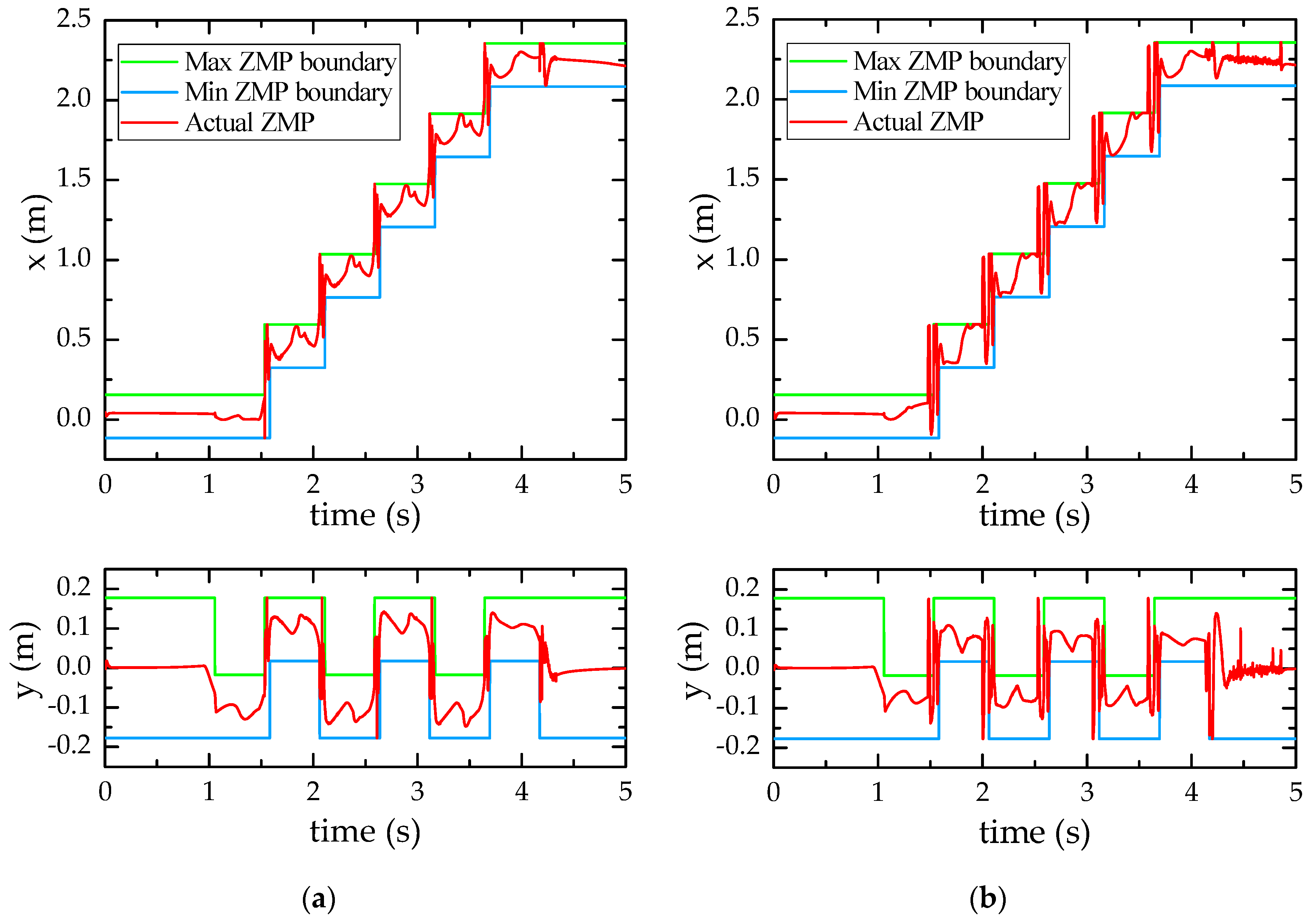
Firstly we have compared the ZMP following-up performances in Case 1 and Case 2, and the results are shown in Figure 5. The swing legs in Case 1 and Case 2 are planned in the same way, but the ZMP compensation is only performed in Case 1. In Case 2, the actual ZMP in the x direction is affected strongly by the motion of the swing leg: in the first half of the single-support phase of each step, the actual ZMP approaches the rear edge of the support rectangle, but in the latter half, it quickly moves to the front edge of the support rectangle and sometimes goes beyond it; and in the y direction, the swing leg has similar effects on the ZMP. The swing leg in Case 2 applies an additional torque in the roll direction to the trunk due to its gravity once it is off the ground, which biases the actual ZMP toward the inner edge of the support rectangle. Eventually, the swing leg touches the ground in advance, and the sole collides with the ground, causing the ZMP trajectory fluctuate drastically in double-support phase. While in case 1, the robot has a higher stability benefitting from the ZMP compensation. Whether in the x direction or the y direction, the actual ZMP trajectory is closer to the center line of the support rectangle and keeps itself inside the support polygon all the time. Therefore, the landing is smoother and the resulting impact force is smaller, which lead to smaller fluctuation in the ZMP trajectory.

Secondly, we have compared the moments required to walk as planned in Case 1 and Case 3. Case 1 and Case 3 differ in the planning method of the swing leg in x direction: Case 1 uses the friction constraint method proposed in this paper, while Case 3 uses the traditional quartic interpolation method. In order to ensure there is no slip occurring, we set the ground friction coefficient to be 2 and then examine the moment between the support leg and the ground during walking. Figure 6 shows the moment between the sole and ground in a single-support phase. It keeps within the permissible range in Case 1, but it is outside the permissible range from time to time in Case 3. The permissible range is calculated under the condition that ${\mu }_s=0.75$ based on Equation (10). The results mean that in a single-support phase, friction moment provided by the ground is large enough to prevent rotational slip in Case 1, but in Case 3, the friction moment is not.

Finally, Figure 7 shows the yaw angles of the robot during travel in all the 4 cases, which are measured by the IMU. In Case 1, the maximum yaw angle of the robot is 0.36°, and the yaw angle at the last stop is −0.16°. Such a small yaw angle is negligible, indicating that the robot has almost no rotational slip during the whole motion. In Case 2, the robot shows a noticeable rotational slip and the maximum yaw angle and the final yaw angle are both −1.93°. The reason for this can be found from the ZMP trajectory in Figure 5b: the ZMP stability margin is low, the robot cannot always maintain the planned posture, and there is a tendency to roll and tilt forward and backward. In addition, the swing leg touches the ground in advance and collides with the ground. The shock caused by the collision does not stop, even when the double-support phase ends. Therefore, the sole of the support leg does not always fit the ground: sometimes only its edge hits the ground, and sometimes only its tip touches the ground. So the required friction can’t be provided, and the robot rotates with the swinging of the swing leg. In Case 3, the maximum yaw angle is −1.66° and the final yaw angle is −1.35°. The reason is that the planned trajectory cannot satisfy the frictional constraint between the sole and the ground all the time, which can be deduced in the curve for Case 3 in Figure 6. In Case 4, because the problems similar to those in Case 2 and Case 3 exist at the same time, the robot walks in an extremely unstable manner. The maximum yaw angle reaches −5.36°, and the final yaw angle is −3.47° in this case, which is very dangerous for real robots, since the number of walking steps is small in the simulation compared to the real walking situation.

From more simulation experiments, we found that when the ratio of leg’s mass to the total mass of the robot is larger than one sixth, slip is the key factor of restricting the walking speed. The performance of our method was outstanding compared with the conventional methods. However, if the ratio of the leg’s mass to the total mass of the robot was smaller than one sixth, our method shows no advantages. Maybe some factors other than slip are more significant. As we know, most of the existing humanoid robots belong to the former. So our method is suitable for improving most of robots’ performances in fast walking.

6. Conclusions

In order to increase walking speed of the humanoid robot, it is necessary to increase the driving power of the leg joints, which in turn leads to an increase of leg weight. This paper aims to overcome the rotational slip of a motor-driven high-power humanoid robot during its fast walking through a gait planning algorithm with free joints of the waist and arms for multitasking during walking. The main contributions are as follows. Firstly, a 3D three-mass model applicable to fast-walking robots with heavy legs was proposed. Then based on this model, the maximum moment provided by the ground friction during walking was calculated, which was then used as a constraint to plan the swing leg motion. After that, the influence of the swing leg on ZMP was calculated, and thus the original reference ZMP trajectory was compensated for to obtain a new one. Based on the compensated ZMP trajectory, the preview control method was adopted to plan the trajectory of the CoM of the inverted pendulum. Finally, the trajectories of all the joints of the legs could be obtained by inverse kinematics.

In this paper, the effectiveness of the proposed algorithm was verified by simulation, and the conclusions are as follows.

1)

For a humanoid robot with heavy legs, it is the motion of the swing leg that causes rotational slip and strongly affects the overall ZMP of the robot;

2)

By using the friction constraint method proposed in this paper to plan the swing leg motion, the maximum walking speed without rotating slip can be obtained;

3)

If the ZMP variation caused by the swing leg motion is compensated to the reference ZMP, the actual ZMP of the robot will follow the reference ZMP better, as a result the robot maintains its posture better and the leg lands more stably, avoiding the rotational slip caused by the sole not being attached to the ground;

4)

We can only obtain a fast walking gait without rotational slip if we use both the friction constraint method and the ZMP compensation method proposed in this paper sequentially.

Looking towards future work, some research needs to evolve the off-line methods proposed in this paper to on-line methods, while other research needs to apply these methods to real robots. Since there are model errors between the actual robot and the simulation model, the motors have servo error, and the ground is not an ideal plane, a series of engineering problems in application need to be solved. Furthermore, if the walking distance is long, there will be an accumulation of errors, which means a stability control method is required.

References

1. Kajita, S.; Hirukawa, H.; Harada, K.; Yokoi, K. Introduction to Humanoid Robotics; Springer: Berlin/Heidelberg, Germany, 2014. [Google Scholar]
2. Ikeda, H.; Kawabe, T.; Wada, R.; Sato, K. Step-climbing tactics using a mobile robot pushing a hand cart. Appl. Sci. Basel 2018, 8, 2114. [Google Scholar] [CrossRef]
3. Zhao, J.; Gao, J.; Zhao, F.; Liu, Y. A search-and-rescue robot system for remotely sensing the underground coal mine environment. Sensors 2017, 17, 2426. [Google Scholar] [CrossRef] [PubMed]
4. Hirai, K.; Hirose, M.; Haikawa, Y.; Takenaka, T. The development of Honda humanoid robot. In Proceedings of the 1998 IEEE International Conference on Robotics and Automation (Cat. No.98CH36146), Leuven, Belgium, 20 May 1998; Volume 1622, pp. 1322–1326. [Google Scholar]
5. Yu, Z.; Huang, Q.; Ma, G.; Chen, X.; Zhang, W.; Li, J.; Gao, J. Design and development of the humanoid robot BHR-5. Adv. Mech. Eng. 2014, 6, 852937. [Google Scholar] [CrossRef]
6. Kaneko, K.; Kaminaga, H.; Sakaguchi, T.; Kajita, S.; Morisawa, M.; Kumagai, I.; Kanehiro, F. Humanoid Robot HRP-5P: An electrically actuated humanoid robot with high-power and wide-range joints. IEEE Robot. Automat. Lett. 2019, 4, 1431–1438. [Google Scholar] [CrossRef]
7. Feng, S.; Xinjilefu, X.; Atkeson, C.G.; Kim, J. Optimization based controller design and implementation for the Atlas robot in the DARPA Robotics Challenge Finals. In Proceedings of the 2015 IEEE-RAS 15th International Conference on Humanoid Robots (Humanoids), Seoul, Korea, 3–5 November 2015; pp. 1028–1035. [Google Scholar]
8. Jeong, H.; Oh, J.; Kim, M.; Joo, K.; Kweon, I.S. Control strategies for a humanoid robot to drive and then egress a utility vehicle for remote approach. In Proceedings of the 2015 IEEE-RAS 15th International Conference on Humanoid Robots (Humanoids), Seoul, Korea, 3–5 November 2015; pp. 811–816. [Google Scholar]
9. BostonDynamics. Parkour Atlas. Available online: https://www.youtube.com/watch?v=LikxFZZO2sk (accessed on 11 October 2018).
10. Raibert, M. Dynamic legged robots for rough terrain. In Proceedings of the 2010 10th IEEE-RAS International Conference on Humanoid Robots, Nashville, TN, USA, 6–8 December 2010; p. 1. [Google Scholar]
11. Takahiro, H.; Barkan, U.; Atsuo, K.; Chi, Z. Yaw moment compensation of biped fast walking using 3D inverted pendulum. In Proceedings of the 2008 10th IEEE International Workshop on Advanced Motion Control, Trento, Italy, 26–28 March 2008; pp. 296–300. [Google Scholar]
12. Ugurlu, B.; Saglia, J.; Tsagarakis, N.; Caldwell, D. Yaw moment compensation for bipedal robots via intrinsic angular momentum constraint. Int. J. Human. Robot. 2012, 9, 1250033. [Google Scholar] [CrossRef]
13. Yang, L.; Liu, Z.; Zhang, Y. Energy-efficient yaw moment control for humanoid robot utilizing arms swing. Int. J. Precis. Eng. Manufact. 2016, 17, 1121–1128. [Google Scholar] [CrossRef]
14. Collins, S.H.; Adamczyk, P.G.; Kuo, A.D. Dynamic arm swinging in human walking. Proc. R. Soc. B Biol. Sci. 2009, 276, 3679–3688. [Google Scholar] [CrossRef] [PubMed] [Green Version]
15. Xing, D.; Su, J. Arm/trunk motion generation for humanoid robot. Sci. China Inf. Sci. 2010, 53, 1603–1612. [Google Scholar] [CrossRef]
16. Xing, D.; Su, J. Motion generation for the upper body of humanoid roBOT. Int. J. Human. Robot. 2010, 7, 281–294. [Google Scholar] [CrossRef]
17. Cisneros, R.; Benallegue, M.; Morisawa, M.; Yoshida, E.; Yokoi, K.; Kanehiro, F. Partial yaw moment compensation using an optimization-based multi-objective motion solver. In Proceedings of the 2018 IEEE-RAS 18th International Conference on Humanoid Robots (Humanoids), Beijing, China, 6–9 November 2018; pp. 1017–1024. [Google Scholar]
18. Cisneros, R.; Benallegue, M.; Benallegue, A.; Morisawa, M.; Audren, H.; Gergondet, P.; Escande, A.; Kheddar, A.; Kanehiro, F. Robust humanoid control using a QP Solver with integral gains. In Proceedings of the 2018 IEEE/RSJ International Conference on Intelligent Robots and Systems (IROS), Madrid, Spain, 1–5 October 2018; pp. 7472–7479. [Google Scholar]
19. Kajita, S.; Benallegue, M.; Cisneros, R.; Sakaguchi, T.; Nakaoka, S.; Morisawa, M.; Kaminaga, H.; Kumagai, I.; Kaneko, K.; Kanehiro, F. Biped gait control based on spatially quantized dynamics. In Proceedings of the 2018 IEEE-RAS 18th International Conference on Humanoid Robots (Humanoids), Beijing, China, 6–9 November 2018; pp. 75–81. [Google Scholar]
20. Huang, Q.; Yokoi, K.; Kajita, S.; Kaneko, K.; Arai, H.; Koyachi, N.; Tanie, K. Planning walking patterns for a biped robot. IEEE Trans. Robot. Automat. 2001, 17, 280–289. [Google Scholar] [CrossRef]
21. Kajita, S.; Kanehiro, F.; Kaneko, K.; Fujiwara, K.; Harada, K.; Yokoi, K.; Hirukawa, H. Biped walking pattern generation by using preview control of zero-moment point. In Proceedings of the 2003 IEEE International Conference on Robotics and Automation (Cat. No.03CH37422), Taipei, Taiwan, 14–19 September 2003; Volume 1622, pp. 1620–1626. [Google Scholar]
22. Park, J.H.; Kim, K.D. Biped robot walking using gravity-compensated inverted pendulum mode and computed torque control. In Proceedings of Proceedings of the 1998 IEEE International Conference on Robotics and Automation (Cat. No.98CH36146), Leuven, Belgium, 20 May 1998; Volume 3524, pp. 3528–3533. [Google Scholar]
23. Sato, T.; Sakaino, S.; Ohnishi, K. Real-time walking trajectory generation method at constant body height in single support phase for three-dimensional biped robot. In Proceedings of the 2009 IEEE International Conference on Industrial Technology, Gippsland, VIC, Australia, 10–13 February 2009; pp. 1–6. [Google Scholar]
24. Sato, T.; Sakaino, S.; Ohnishi, K. Real-time walking trajectory generation method with three-mass models at constant body height for three-dimensional biped robots. IEEE Trans. Ind. Electron. 2011, 58, 376–383. [Google Scholar] [CrossRef]
25. Zhu, C.; Kawamura, A. What is the real frictional constraint in biped walking? Discussion on frictional slip with rotation. In Proceedings of the 2006 IEEE/RSJ International Conference on Intelligent Robots and Systems, Beijing, China, 9–15 October 2006; pp. 5762–5768. [Google Scholar]
26. Takabayashi, Y.; Ishihara, K.; Yoshioka, M.; Liang, H.; Liu, C.; Zhu, C. Frictional constraints on the sole of a biped robot when slipping. In Proceedings of the 2017 IEEE/RSJ International Conference on Intelligent Robots and Systems (IROS), Vancouver, BC, Canada, 24–28 September 2017; pp. 5011–5016. [Google Scholar]
Figure 1. Typical motor-driven humanoid robot. They always have an inertial measurement unit (IMU) fixed inside the chest and a six-dimensional force-torque (F-T) sensor for each ankle. Each leg has 6 degrees of freedom (DoFs): (a) Simulation model; (b) DoF configuration.
Applsci 09 02657 g001
Figure 2. 3D three-mass model. The robot is divided into 3 parts: the inverted pendulum, the swing leg and the support leg. There is no kinematic constraint between the legs and the inverted pendulum. Z M P p e n d and Z M P t o t a l represent the zero-moment point (ZMP) of the inverted pendulum and the whole robot respectively. x ,   ¨   y ¨   a n d   z ¨ represent the accelerations of the center of mass in three directions, respectively.
Applsci 09 02657 g002
Figure 3. Setting of the landing points p 1 ,   p 2 ,   ,   p N   , which represent ZMPs for an inverted pendulum and determine the walking length L x and width L y . The rectangles represent the robot’s footprints.
Applsci 09 02657 g003
Figure 4. Snapshots of biped walking in Case 1. The robot walks straightly along the center line all the time stably.
Applsci 09 02657 g004
Figure 5. ZMP trajectory. The actual ZMP is calculated based on the data measured by the six-dimensional F-T sensor. The ZMP boundary is the boundary of the sole of the support leg. (a) Case 1; (b) Case 2. The ZMP trajectories are nearer to the boundaries in Case 2 than in Case 1.
Applsci 09 02657 g005
Figure 6. The moment between the left sole and ground in a single-support phase. The actual moments in Case 1 and Case 3 are measured by the six-dimensional F-T sensor.
Applsci 09 02657 g006
Figure 7. Yaw angle of the robot during walking. It is measured by the IMU. Yaw angle in Case 1 is close to 0. While yaw angles increase in turn in Case 3, Case 2 and Case 4 and they are non-negligible.
Applsci 09 02657 g007