Effect of Uncertainty in Localized Imperfection on the Ultimate Compressive Strength of Cold-Formed Stainless Steel Hollow Sections


Abstract
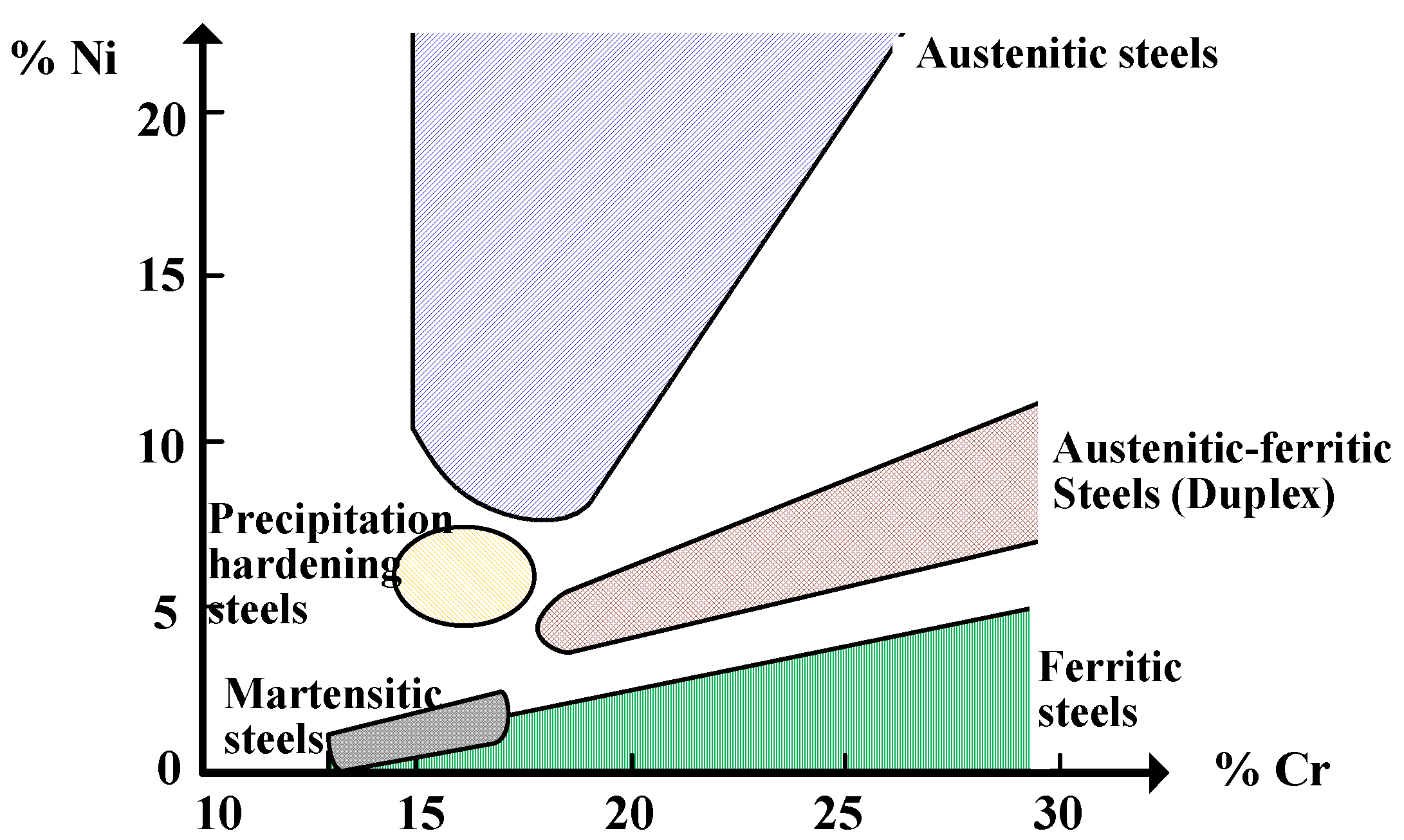
1. Introduction
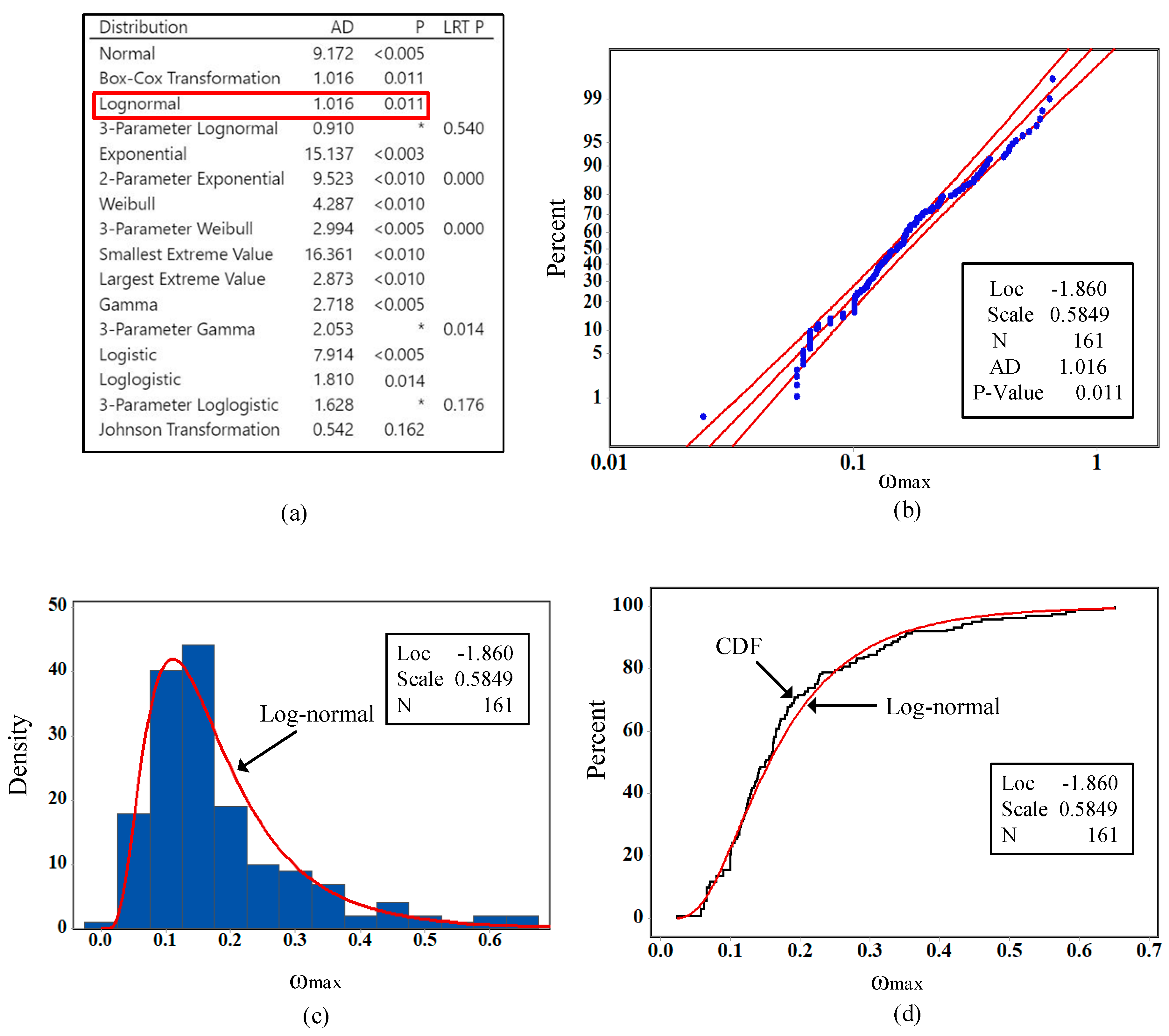
2. Statistical Analysis of the Maximum Localized Imperfection (ω)
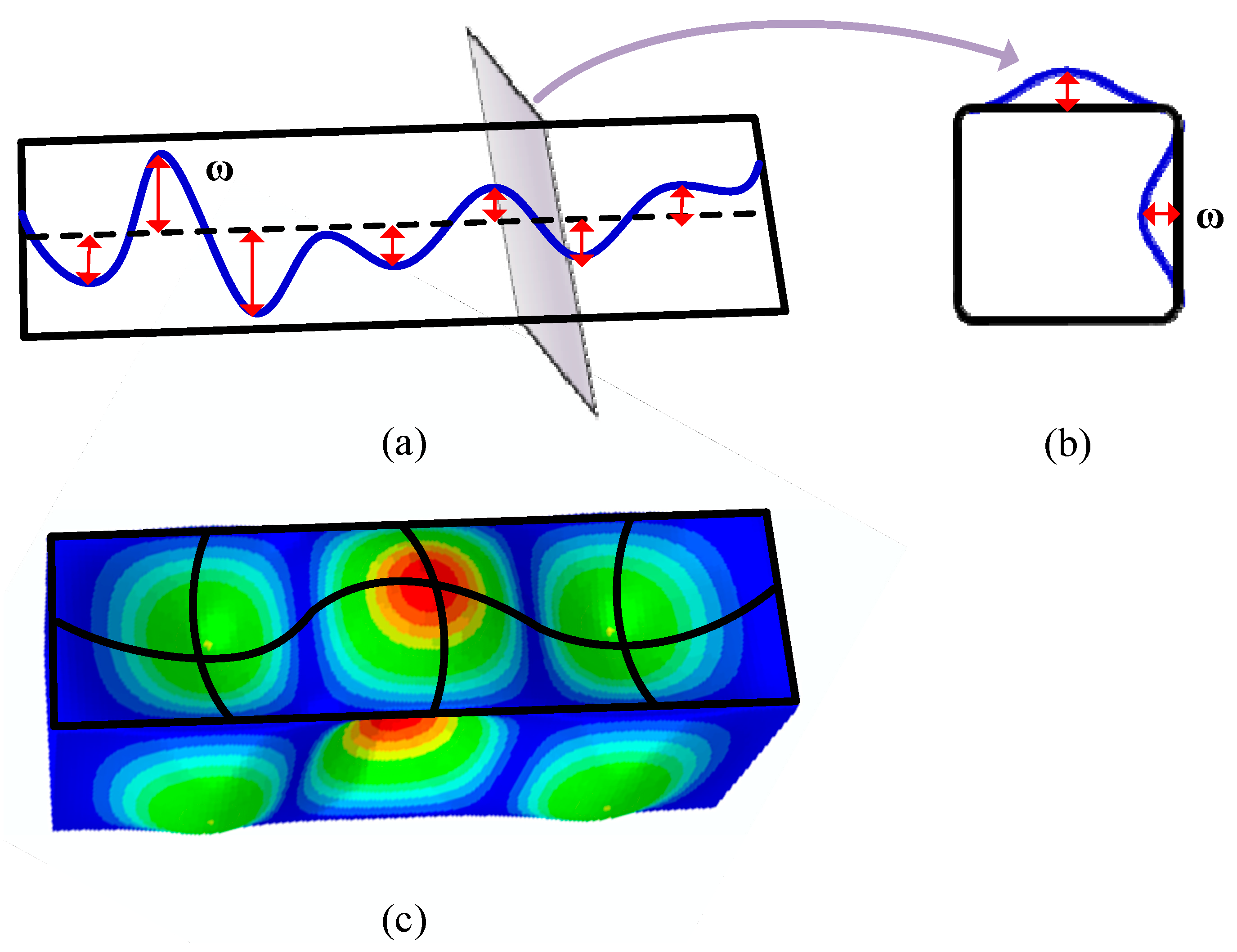
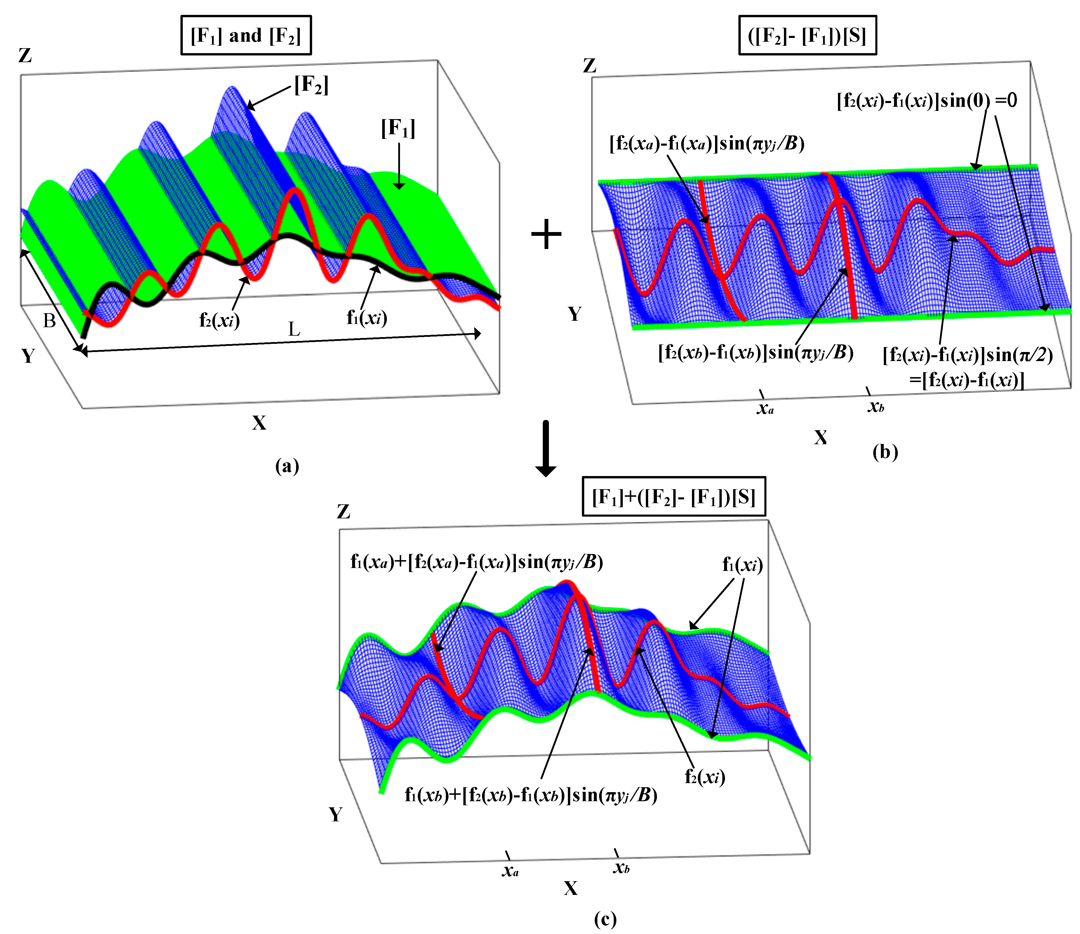
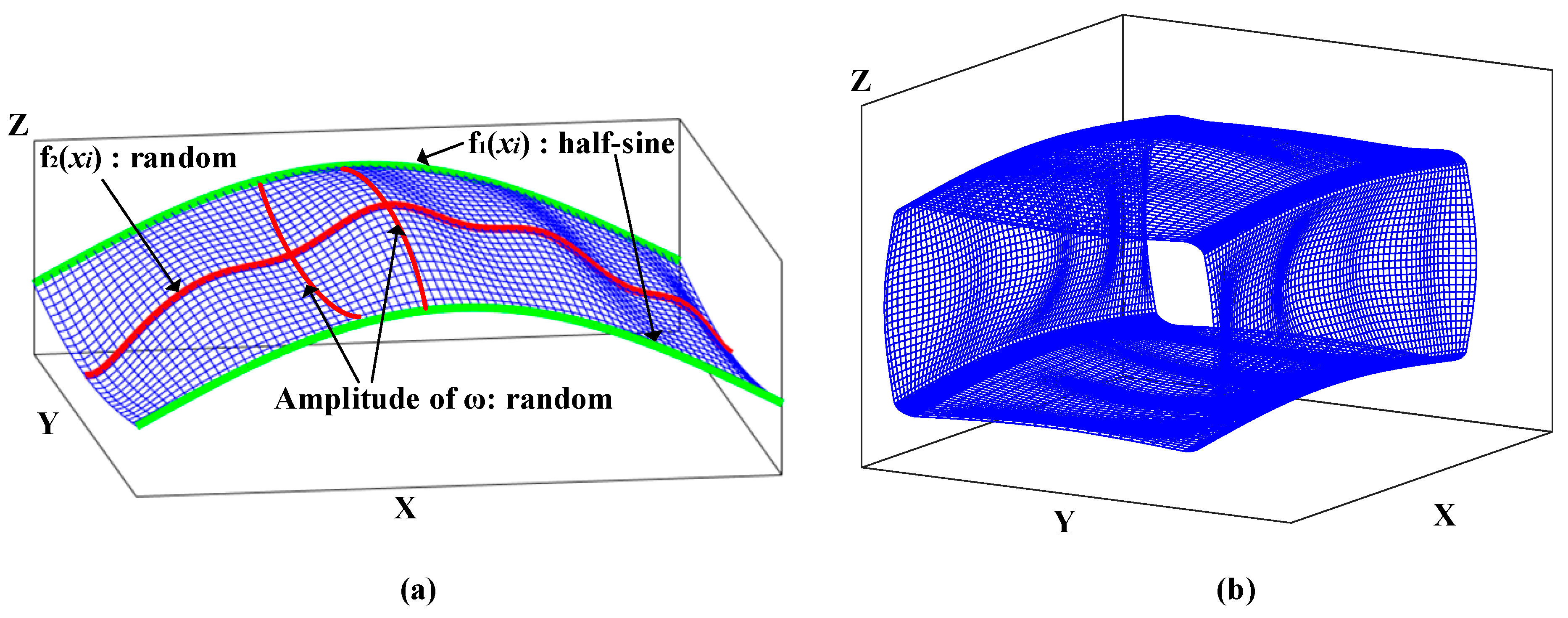
3. Fourier Series-Based 3D Models with Random ω
4. Case Study of Stainless Steel Columns with Cold-Formed RHS and SHS
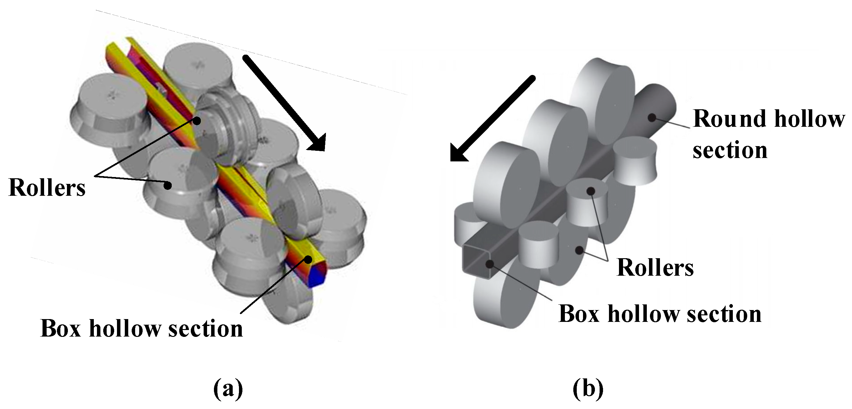
5. Generation of 3D Models of the Studied Columns and Finite Element (FE) Analysis
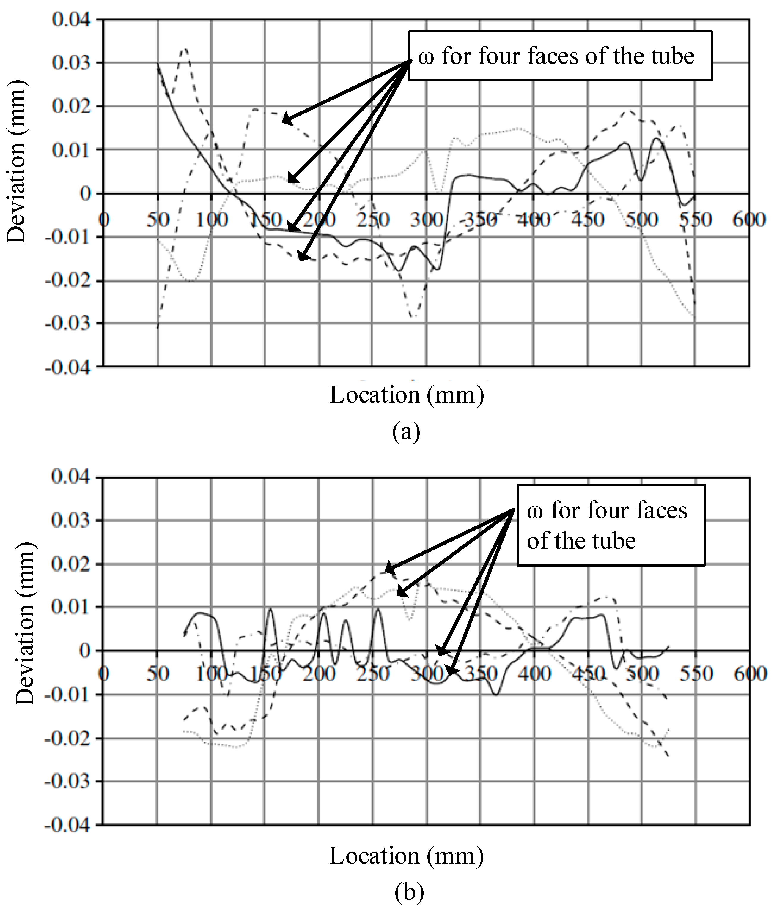
5.1. Generation of 3D Model with Random ω Using MATLAB
5.2. FE Analysis Using ABAQUS
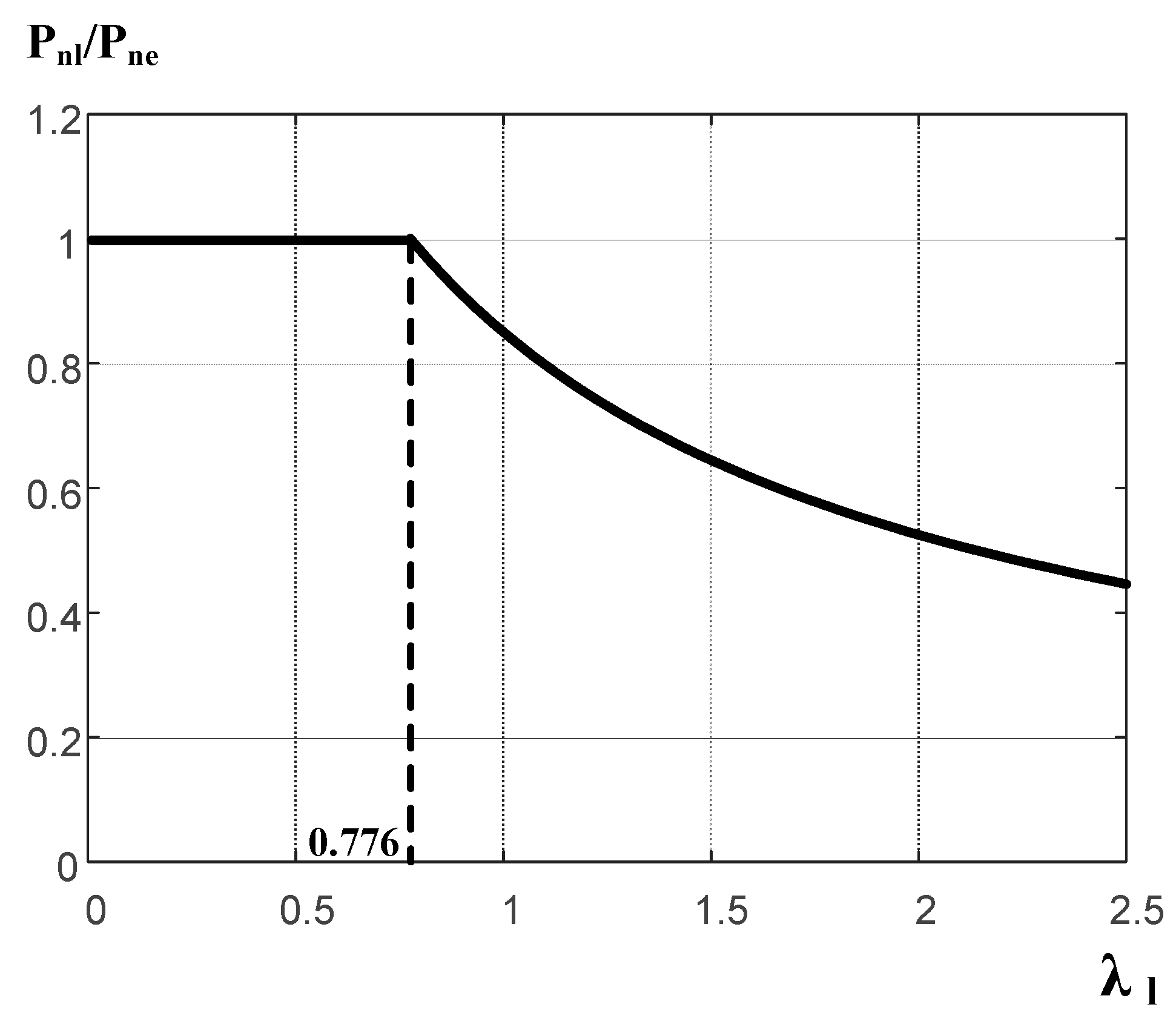
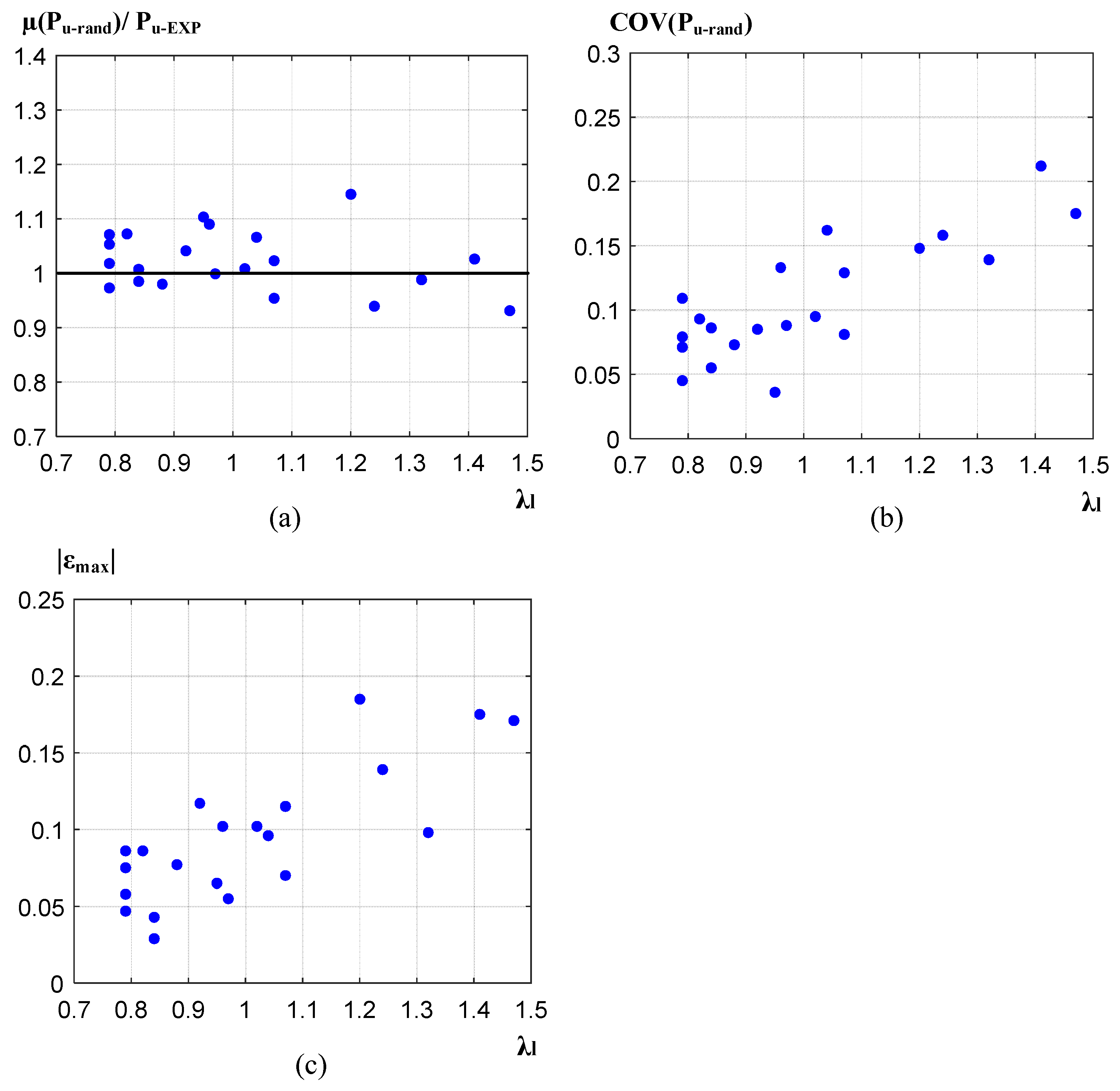
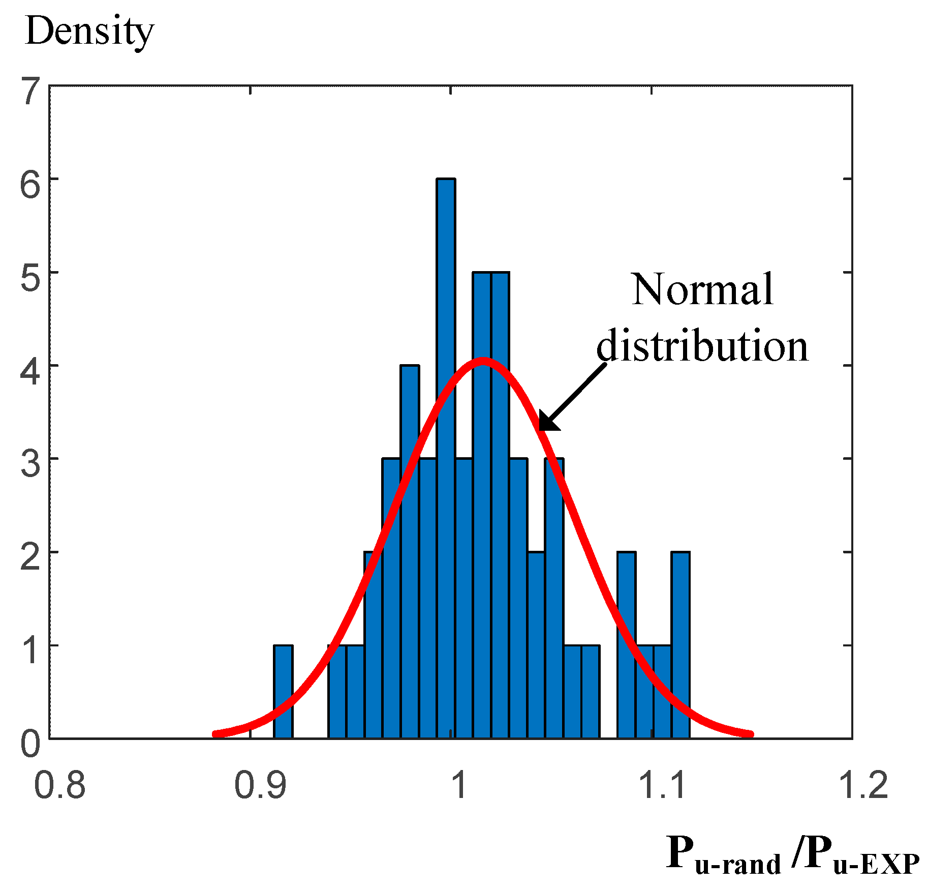
6. Effect of Uncertainty in ω on the Ultimate Compressive Strength of the Studied Columns
7. Conclusions
Author Contributions
Funding
Acknowledgments
Conflicts of Interest
References
- Rossi, B. Discussion on the Use of Stainless Steel in Constructions in View of Sustainability. Thin. Wall. Struct. 2014, 83, 182–189. [Google Scholar] [CrossRef]
- Zitelli, C.; Paolo Folgarait, P.; Schino, A.D. Laser Powder Bed Fusion of Stainless Steel Grades: A Review. Metals 2019, 9, 731. [Google Scholar] [CrossRef]
- Baddoo, N. Design Guide 27: Structural Stainless Steel; American Institute of Steel Construction (AISC): Chicago, IL, USA, 2013. [Google Scholar]
- Chen, X.M.; Xia, J.W.; Xu, B.; Ma, R.W. Mechanical Performance of Built-Up Columns Composed of Four Cold-Formed Square Steel Tubes. Appl. Sci. 2019, 9, 1204. [Google Scholar] [CrossRef]
- Li, H.T.; Young, B. Design of cold-formed high strength steel tubular sections undergoing web crippling. Thin. Wall. Struct. 2018, 133, 192–205. [Google Scholar] [CrossRef]
- López-Colina, C.; Serrano, M.A.; Lozano, M.; Gayarre, F.L.; Suárez, J. Simplified Models for the Material Characterization of Cold-Formed RHS. Materials 2017, 10, 1043. [Google Scholar] [CrossRef] [PubMed]
- Serrano, M.A.; López-Colina, C.; Gayarre, F.L.; Wilkinson, T.; Suárez, J. The Resistance of Welded Joints of Galvanized RHS Trusses with Different Vent Hole Geometries. Appl. Sci. 2019, 9, 1553. [Google Scholar] [CrossRef]
- Li, H.T.; Young, B. Material properties of cold-formed high strength steel at elevated temperatures. Eng. Struct. 2017, 141, 571–583. [Google Scholar] [CrossRef]
- Li, H.T.; Young, B. Behaviour of cold-formed high strength steel RHS under localised bearing forces. Eng. Struct. 2019, 183, 1049–1058. [Google Scholar] [CrossRef]
- Jo, B.; Okamoto, K.; Kasahara, N. Creep Buckling of 304 Stainless-Steel Tubes Subjected to External Pressure for Nuclear Power Plant Applications. Metals 2019, 9, 536. [Google Scholar] [CrossRef]
- Li, H.T.; Young, B. Cold-formed ferritic stainless steel tubular structural members subjected to concentrated bearing loads. Eng. Struct. 2017, 145, 392–405. [Google Scholar] [CrossRef]
- Peng, Y.; Chu, J.; Jun Dong, J. Compressive Behavior and Constitutive Model of Austenitic Stainless Steel S30403 in High Strain Range. Materials 2018, 11, 1023. [Google Scholar] [CrossRef] [PubMed]
- Corradi, M.; Osofero, A.I.; Borri, A. Repair and Reinforcement of Historic Timber Structures with Stainless Steel—A Review. Metals 2019, 9, 106. [Google Scholar] [CrossRef]
- Yrjola, P.; Saynajakangas, J.; Soderberg, K. Stainless Steel Hollow Sections Handbook; Finnish Constructional Steelwork Association: Helsinki, Finland, 2008. [Google Scholar]
- COPRA Reference Manual; Data M Sheet Metal Solutions GmbH: Valley, Germany, 2014.
- Nagamachi, T.; Nakako, T.; Nakamura, D. Effects of Roll Diameter and Offset on Sectional Shape of Square Steel Pipe Processed by Roll Forming. Mater. Trans. 2011, 52, 2159–2164. [Google Scholar] [CrossRef]
- Gardner, L.; Nethercot, D.A. Numerical Modeling of Stainless Steel Structural Components—A Consistent Approach. J. Struct. Eng. 2004, 130, 1586–1601. [Google Scholar] [CrossRef]
- Wang, J.; Afshan, S.; Schillo, N.; Theofanous, M.; Feldmann, M.; Gardner, L. Material properties and compressive local buckling response of high strength steel square and rectangular hollow sections. Eng. Struct. 2017, 130, 297–315. [Google Scholar] [CrossRef]
- Zhao, O.; Gardner, L.; Young, B. Experimental Study of Ferritic Stainless Steel Tubular Beam-Column Members Subjected to Unequal End Moments. J. Struct. Eng. 2016, 142, 04016091. [Google Scholar] [CrossRef]
- Zhao, O.; Rossi, B.; Gardner, L.; Young, B. Behaviour of structural stainless steel cross-sections under combined loading - Part I: Experimental study. Eng. Struct. 2015, 89, 236–246. [Google Scholar] [CrossRef]
- Young, B.; Lui, W.M. Behavior of Cold-Formed High Strength Stainless Steel Sections. J. Struct. Eng. 2005, 131, 1738–1745. [Google Scholar] [CrossRef]
- Lui, W.M.; Ashraf, M.; Young, B. Tests of cold-formed duplex stainless steel SHS beam–columns. Eng. Struct. 2014, 74, 111–121. [Google Scholar] [CrossRef]
- Li, H.T.; Young, B. Cold-formed high strength steel SHS and RHS beams at elevated temperatures. J. Constr. Steel. Res. 2019, 158, 475–485. [Google Scholar] [CrossRef]
- AISI S100-16 North American Specification for the Design of Cold-Formed Steel Structural Members, 2016th ed.; American Iron and Steel Institute (AISC): Washington, DC, USA, 2016.
- Zheng, B.F.; Shu, G.P.; Xin, L.C.; Yang, R.; Jiang, Q.L. Study on the Bending Capacity of Cold-formed Stainless Steel Hollow Sections. Structures 2016, 8, 63–74. [Google Scholar] [CrossRef]
- Arrayago, I.; Real, E.; Mirambell, E. Experimental study on ferritic stainless steel RHS and SHS beam-columns. Thin. Wall. Struct. 2016, 100, 93–104. [Google Scholar] [CrossRef]
- Theofanous, M.; Gardner, L. Testing and numerical modelling of lean duplex stainless steel hollow section columns. Eng. Struct. 2009, 31, 3047–3058. [Google Scholar] [CrossRef]
- Huang, Y.; Young, B. Tests of pin-ended cold-formed lean duplex stainless steel columns. J. Constr. Steel. Res. 2013, 82, 203–215. [Google Scholar] [CrossRef]
- Afshan, S.; Gardner, L. Experimental Study of Cold-Formed Ferritic Stainless Steel Hollow Sections. J. Struct. Eng. 2013, 139, 717–728. [Google Scholar] [CrossRef]
- Bock, M.; Arrayago, I.; Real, E. Experiments on cold-formed ferritic stainless steel slender sections. J. Constr. Steel. Res. 2015, 109, 13–23. [Google Scholar] [CrossRef]
- Arrayago, I.; Real, E. Experimental Study on Ferritic Stainless Steel RHS and SHS Cross-sectional Resistance Under Combined Loading. Structures 2015, 4, 69–79. [Google Scholar] [CrossRef]
- Minitab 18 Reference Manual; Minitab, LLC: State College, PA, USA, 2019.
- JG/T 178-2005 Cold-Formed Steel Hollow Sections for Building Structures; Standards Press of China: Beijing, China, 2005.
- CEN, EN-10219-2:2006 Cold Formed Welded Structural Hollow Sections of Non-Alloy and Fine Grain Steels. Part 2: Tolerances, Dimensions and Sectional Properties; European Committee for Standardization: Brussels, Belgium, 2006.
- Davis, J.C. Statistics and Data Analysis in Geology, 3rd ed.; Wiley & Sons: New York, NY, USA, 1973. [Google Scholar]
- Higgins, J.R. Sampling Theory in Fourier and Signal Analysis: Foundations, 1st ed.; Clarendon Press: Oxford, UK, 1996. [Google Scholar]
- Young, B.; Lui, W.M. Tests of cold-formed high strength stainless steel compression members. Thin. Wall. Struct. 2006, 44, 224–234. [Google Scholar] [CrossRef]
- Young, B.; Liu, Y.H. Experimental Investigation of Cold-Formed Stainless Steel Columns. J. Struct. Eng. 2003, 129, 169–176. [Google Scholar] [CrossRef]
- Gardner, L.; Nethercot, D.A. Experiments on stainless steel hollow sections-Part 2: Member behavior of columns and beams. J. Constr. Steel. Res. 2004, 60, 1319–1332. [Google Scholar] [CrossRef]
- Arrayago, I.; Rasmussen, K.J.R.; Real, E. Full slenderness range DSM approach for stainless steel hollow cross-sections. J. Constr. Steel. Res. 2017, 133, 156–166. [Google Scholar] [CrossRef]
- Arrayago, I.; Rasmussen, K.J.R.; Real, E. Full slenderness range DSM approach for stainless steel hollow cross-section columns and beam-columns. J. Constr. Steel. Res. 2017, 138, 246–263. [Google Scholar] [CrossRef]
- Abaqus, v. 6.13 Reference Manual; Simulia, Dassault Systemes: Johnston, RI, USA, 2013. [Google Scholar]
- MATLAB 2017(b) Reference Manual; The MathWorks: Natick, MA, USA, 2019.
- Riks, E. An incremental approach to the solution of snapping and buckling problems. Int. J. Solids Struct. 1979, 15, 529–551. [Google Scholar] [CrossRef]
- Jandera, M.; Machacek, J. Residual stress influence on material properties and column behavior of stainless steel SHS. Thin. Wall. Struct. 2014, 83, 12–18. [Google Scholar] [CrossRef]


| Reference | Stainless Steel Groups | Grade | No. of Samples with Measured ω |
|---|---|---|---|
| B.F. Zheng et al., 2016 [25] | Austenitic | EN1.4301 | 4 |
| I. Arrayago. et al., 2016 [26] | Ferritic | EN1.4003 | 12 |
| B. Young and W.M. Lui, 2005 [21] | Duplex | EN1.4162 | 5 |
| O. Zhao et al., 2015 [20] | Austenitic | EN1.4301 | 10 |
| Austenitic | EN1.4571 | 6 | |
| Austenitic | EN1.4307 | 6 | |
| Austenitic | EN1.4404 | 6 | |
| Duplex | EN1.4162 | 6 | |
| M. Theofanous and L. Gardner, 2009 [27] | Duplex | EN1.4162 | 8 |
| W.M. Lui et al., 2014 [22] | Duplex | EN1.4462 | 10 |
| Y. Huang and B. Young, 2013 [28] | Duplex | EN1.4162 | 22 |
| S. Afshan and L. Gardner, 2013 [29] | Ferritic | EN1.4003 | 6 |
| Ferritic | EN1.4509 | 2 | |
| M. Bock et al., 2015 [30] | Ferritic | EN1.4003 | 8 |
| I. Arrayago and E. Real, 2015 [31] | Ferritic | EN1.4003 | 26 |
| O. Zhao et al., 2016 [19] | Ferritic | EN1.4003 | 24 |
| Total: 161 |
| Reference | Specimen | b1 (mm) | b2 (mm) | t (mm) | R (mm) | L (mm) | λc | λl | ωg |
|---|---|---|---|---|---|---|---|---|---|
| [37] | SHS2L300 | 50.1 | 50.3 | 1.58 | 2.8 | 300 | 0.14 | 0.8 | - |
| RHS1L3000 | 140.1 | 79.9 | 3.01 | 10.0 | 3000 | 0.71 | 0.9 | 0.927 | |
| [28] | C5L200 | 100.1 | 50.1 | 2.5 | 3.7 | 200 | 0.18 | 1.0 | - |
| C6L200 | 150.0 | 50.1 | 2.5 | 4.3 | 200 | 0.18 | 1.5 | - | |
| C6L550 | 150.1 | 50.2 | 2.49 | 4.5 | 550 | 0.48 | 1.4 | 0.5 | |
| C5L900R | 100.1 | 50.4 | 2.49 | 3.5 | 900 | 0.79 | 0.8 | 0.857 | |
| C6L900 | 150.4 | 50.3 | 2.47 | 4.7 | 900 | 0.79 | 1.3 | 0.857 | |
| C6L1200 | 149.9 | 50.5 | 2.46 | 4.5 | 1200 | 1.04 | 1.2 | 1.143 | |
| C6L1550 | 150.5 | 50.3 | 2.49 | 4.5 | 1550 | 1.35 | 1.0 | 1.476 | |
| [29] | RHS 120 × 80 × 3-SC2 | 120.0 | 80.0 | 2.83 | 6.7 | 362 | 0.16 | 0.82 | - |
| RHS 120 × 80 × 3-1077 | 120.0 | 79.9 | 2.87 | 6.8 | 1077 | 0.35 | 0.8 | 0.95 | |
| RHS 120 × 80 × 3-1577 | 120.0 | 79.9 | 2.81 | 6.4 | 1577 | 0.51 | 0.8 | 0.96 | |
| [38] | R1L1200 | 120.1 | 40.1 | 1.94 | 5.0 | 1199 | 0.48 | 1.1 | 0.254 |
| R1L2000 | 120.2 | 40.0 | 1.95 | 5.1 | 2000 | 0.80 | 1.0 | 0.444 | |
| R3L2000 | 120.0 | 80.0 | 2.80 | 6.7 | 2000 | 0.44 | 0.8 | 0.381 | |
| [39] | SHS100 × 100 × 2-LC-2 m | 99.8 | 99.9 | 1.86 | 3.2 | 2000 | 0.73 | 1.0 | 0.1 |
| RHS100 × 50 × 2-LCJ-2 m | 99.8 | 49.8 | 1.83 | 3.7 | 2000 | 0.80 | 0.9 | 0.6 | |
| RHS100 × 50 × 2-LC-1 m | 99.8 | 50.0 | 1.82 | 3.6 | 1000 | 0.69 | 1.0 | 0.1 | |
| RHS120 × 80 × 3-LC-1 m | 120.0 | 80.2 | 2.86 | 5.7 | 1001 | 0.45 | 0.8 | 1 | |
| [21] | 160 × 80 × 3 | 160.1 | 80.8 | 2.87 | 9.0 | 600 | 0.09 | 1.2 | - |
| 200 × 110 × 4 | 196.2 | 108.5 | 4.01 | 13.0 | 600 | 0.07 | 1.1 | - |
| Specimen | λl | Pu-EXP (kN) | µ(Pu-rand) (kN) | µ(Pu-rand) /Pu-EXP | COV(Pu-rand) | |εmax| |
|---|---|---|---|---|---|---|
| SHS2L300 | 0.84 | 175.7 | 177.8 | 0.985 | 0.086 | 0.043 |
| RHS1L3000 | 0.88 | 513.5 | 454.7 | 0.980 | 0.073 | 0.077 |
| C5L200 | 0.95 | 370.1 | 387.5 | 1.103 | 0.036 | 0.065 |
| C6L200 | 1.47 | 404.1 | 413.2 | 0.931 | 0.175 | 0.171 |
| C6L550 | 1.41 | 353.2 | 388.1 | 1.026 | 0.212 | 0.175 |
| C5L900R | 0.84 | 336.0 | 326.0 | 1.007 | 0.055 | 0.029 |
| C6L900 | 1.32 | 333.5 | 345.2 | 0.988 | 0.139 | 0.098 |
| C6L1200 | 1.20 | 284.5 | 300.7 | 1.142 | 0.108 | 0.185 |
| C6L1550 | 1.02 | 230.0 | 249.2 | 1.008 | 0.095 | 0.102 |
| RHS 120 × 80 × 3-SC2 | 0.82 | 441.0 | 434.2 | 1.072 | 0.093 | 0.086 |
| RHS 120 × 80 × 3-1077 | 0.79 | 463.0 | 432.1 | 1.018 | 0.109 | 0.075 |
| RHS 120 × 80 × 3-1577 | 0.79 | 382.0 | 401.5 | 0.973 | 0.045 | 0.058 |
| R1L1200 | 1.07 | 167.0 | 153.5 | 1.02 | 0.129 | 0.115 |
| R1L2000 | 0.97 | 141.3 | 137.9 | 0.999 | 0.088 | 0.055 |
| R3L2000 | 0.79 | 394.0 | 355.7 | 1.071 | 0.071 | 0.047 |
| SHS100 × 100 × 2-LC-2 m | 1.04 | 176.0 | 183.0 | 1.066 | 0.162 | 0.096 |
| RHS100 × 50 × 2-LCJ-2 m | 0.92 | 157.0 | 145.3 | 1.041 | 0.085 | 0.117 |
| RHS100 × 50 × 2-LC-1 m | 0.96 | 163.0 | 151.4 | 1.090 | 0.133 | 0.102 |
| RHS120 × 80 × 3-LC-1 m | 0.79 | 448.0 | 415.5 | 1.053 | 0.079 | 0.086 |
| 160 × 80 × 3 | 1.24 | 537.3 | 505.0 | 0.939 | 0.158 | 0.139 |
| 200 × 110 × 4 | 1.07 | 957.0 | 928.0 | 0.958 | 0.081 | 0.070 |
© 2019 by the authors. Licensee MDPI, Basel, Switzerland. This article is an open access article distributed under the terms and conditions of the Creative Commons Attribution (CC BY) license (http://creativecommons.org/licenses/by/4.0/).
Share and Cite
Shen, Y.; Chacón, R. Effect of Uncertainty in Localized Imperfection on the Ultimate Compressive Strength of Cold-Formed Stainless Steel Hollow Sections. Appl. Sci. 2019, 9, 3827. https://doi.org/10.3390/app9183827
Shen Y, Chacón R. Effect of Uncertainty in Localized Imperfection on the Ultimate Compressive Strength of Cold-Formed Stainless Steel Hollow Sections. Applied Sciences. 2019; 9(18):3827. https://doi.org/10.3390/app9183827
Chicago/Turabian StyleShen, Yanfei, and Rolando Chacón. 2019. "Effect of Uncertainty in Localized Imperfection on the Ultimate Compressive Strength of Cold-Formed Stainless Steel Hollow Sections" Applied Sciences 9, no. 18: 3827. https://doi.org/10.3390/app9183827
APA StyleShen, Y., & Chacón, R. (2019). Effect of Uncertainty in Localized Imperfection on the Ultimate Compressive Strength of Cold-Formed Stainless Steel Hollow Sections. Applied Sciences, 9(18), 3827. https://doi.org/10.3390/app9183827