On Video Analysis of Omnidirectional Bee Traffic: Counting Bee Motions with Motion Detection and Image Classification

Abstract

Omnidirectional bee traffic is the number of bees moving in arbitrary directions in close proximity to the landing pad of a given hive over a given period of time. Video bee traffic analysis has the potential to automate the assessment of omnidirectional bee traffic levels, which, in turn, may lead to a complete or partial automation of honeybee colony health assessment. In this investigation, we proposed, implemented, and partially evaluated a two-tier method for counting bee motions to estimate levels of omnidirectional bee traffic in bee traffic videos. Our method couples motion detection with image classification so that motion detection acts as a class-agnostic object location method that generates a set of regions with possible objects and each such region is classified by a class-specific classifier such as a convolutional neural network or a support vector machine or an ensemble of classifiers such as a random forest. The method has been, and is being iteratively field tested in BeePi monitors, multi-sensor electronic beehive monitoring systems, installed on live Langstroth beehives in real apiaries. Deployment of a BeePi monitor on top of a beehive does not require any structural modification of the beehive’s woodenware, and is not disruptive to natural beehive cycles. To ensure the replicability of the reported findings and to provide a performance benchmark for interested research communities and citizen scientists, we have made public our curated and labeled image datasets of 167,261 honeybee images and our omnidirectional bee traffic videos used in this investigation.

Dataset: The three image datasets (BEE1, BEE2_1S and BEE2_2S) used in this investigation are publicly available at https://usu.box.com/s/0a5yurmn7ija15cp236awa1re65mbcnr, https://usu.box.com/s/p7y8v95ot9u9jvjbbayci61no3lzbgx3 and https://usu.box.com/s/3ccizd5b1qzcqcs4t0ivawmrxbgva7ym, respectively. The omnidirectional bee traffic videos and the corresponding human bee motion counts are included in the Supplementary Materials.

1. Introduction

Honeybees (Apis mellifera) provide approximately 14% of the overall pollination services in agricultural production [1]. Honeybee traffic, i.e., the number of bees that move in close proximity to a beehive per a given time period, is an important indicator of how bee colonies react to foraging opportunities, weather events, pests, and diseases. For example, pollen supply affects brood rearing rates [2] and worker longevity [3], both of which may, in turn, affect honeybee traffic. Many commercial and amateur beekeepers watch honeybee traffic near their hives to ascertain the state of their colonies, because honeybee traffic carries information on colony behavior and phenology. Honeybee traffic is an indicator of colony exposure to stressors such as failing queens, predatory mites, and airborne toxicants.

While experienced beekeepers can arguably tell which honeybee traffic patterns are produced by stressed colonies, they may not always be physically present to observe them in time to administer appropriate treatment due to fatigue or problems with logistics. The cost of transportation is also a factor, as many beekeepers drive longer distances to their far flung apiaries due to ever increasing urban and suburban sprawl. Insomuch as beekeepers cannot monitor their hives continuously, electronic beehive monitoring (EBM) can help extract valuable information on honeybee colonies without invasive hive inspections or transportation costs [4,5].

Deep learning (DL) and computer vision (CV) have so far remained relatively unexplored in EBM [4,6,7,8,9]). However, several researchers have used both DL and CV in their projects. Rodriguez et al. [10] proposed a system for pose detection and tracking of multiple insects and animals, which they used to monitor the traffic of honeybees and mice. The system uses a deep neural network to detect and associate detected body parts into whole insects or animals. The network predicts a set of 2D confidence maps of present body parts and a set of vectors of part affinity fields that encode associations detected among the parts. Greedy inference is subsequently used to select the most likely predictions for the parts and compiles the parts into larger insects or animals. No details appear to be given on what hive was used in the experiments. From the pictures given in the publication, it appears that the hive used in the experiments is a smaller laboratory hive, not a standard Langstroth or Dadant hive used by many beekeepers worldwide. The system requires a structural modification of the beehive in that a transparent acrylic plastic cover located on top of the ramp ensures the bees remain in the focal plane of the camera. The system uses trajectory tracking to distinguish entering and leaving bees, which works reliably under smaller bee traffic levels. The dataset consists of 100 fully annotated frames, where each frame contains 6–14 honeybees. Since the dataset does not appear to be public, the experimental results cannot be independently replicated.

Babic et al. [11] proposed a system for pollen bearing honeybee detection in surveillance videos obtained at the entrance of a hive. The system’s hardware includes a specially designed wooden box with a raspberry pi camera module inside. The box is mounted on the front side of a standard hive above the hive entrance. There is a glass plate placed on the bottom side of the box, 2 cm above the flight board, which forces the bees entering or leaving the hive to crawl a distance of ≈11 cm. Consequently, the bees in the field of view of the camera cannot fly. The training dataset contains 50 images of pollen bearing honeybees and 50 images of honeybees without pollen. The test dataset consists of 354 honeybee images. Since neither dataset appears to be public, the experimental results cannot be independently replicated.

DL methods have been successfully applied to image classification [12,13,14], speech recognition and audio processing [15,16], music classification and analysis [17,18,19], environmental sound classification [20], and bioinformatics [21,22]. Convolutional neural networks (ConvNets) are DL feedforward neural networks that have been shown to generalize well on large quantities of digital data [23]. In ConvNets, filters of various sizes are convolved with a raw input signal to obtain a stack of filtered signals. This transformation is called a convolutional layer. The size of this layer is equal to the number of convolutional filters. The convolved signals are typically normalized. A standard normalization choice is non-linear activation functions such as the rectified linear unit (ReLU) that converts all negative values to 0s [24,25,26]. The size of the output signal from a layer can be downsampled with a maxpooling layer, where a window is shifted in steps, called strides, across the input signal retaining the maximum value from each window. A fully connected (FC) layer treats a stack of processed signals as a 1D vector so that each value in the output from a previous layer is connected via a synapse (a weighted connection that transmits a value from one unit to another) to each node in the next layer. In addition to these layers, there can be custom layers that implement arbitrary functions to transform signals between consecutive layers.

Krizhevsky, Sutskever, and Hinton [12] did the ground breaking research on applying deep ConvNet architectures to large image datasets that rekindled interest in deep neural networks. The researchers trained a deep ConvNet to classify 1.2 million images in the ImageNet LSVRC-2010 content into 1000 different classes. The network consisted of five convolutional layers, some of which were followed by maxpooling layers, and three FC layers with a final 1000-way softmax layer and dropouts [27] of various rates. The network consisted of 60 million parameters and included 650,000 neurons. Variants of this architecture still dominate the image classification literature and have so far yielded the best results on such publicly available datasets as MNIST [23], CIFAR [28], and ImageNet [29].

A standard way to improve the performance of deep ConvNets is by increasing the number of layers and the number of neurons in each layer. For example, Szegedy et al. [30] proposed a deep ConvNet architecture, called Inception, that improves the utilization of the computational resources inside the network. The architecture is implemented in GoogLeNet, a deep network with 22 layers. This network approximates the expected optimal sparse structure by using dense building blocks available within the network.

A recent development in the state of the art object recognition with ConvNets is the Regions with ConvNets (R-CNN) [31,32]. Given an image, an R-CNN system uses a class-independent object location method (e.g., selective search [33]) to generate a set of region proposals, computes a set of features for each region with a ConvNet, and then classifies these features with a class-specific classifier such as a support-vector machine (SVM) or another ConvNet. YOLO [34] is an object detection system that, instead of applying trained models to multiple locations and scoring them for objects, applies a single neural network to entire images. The network itself divides the image into sub-images and calculates bounding boxes and probabilities for different locations. SSD [35] is another approach to object classification by neural networks that starts with a set of pre-computed, fixed size bounding boxes (called priors) that closely match the distribution of the ground truth object boxes and regresses the priors to the ground truth boxes. Tiny SSD [36] is a recent development of the SSD multi-box approach. It is a deep ConvNet based on SSD for real-time embedded object detection. It is composed of an optimized, non-uniform Fire sub-network stack and a non-uniform sub-network stack of optimized SSD-based auxiliary convolutional feature layers for minimizing model size without negatively affecting object detection performance.

In this article, we contribute to the body of research on object recognition in videos by proposing a two-tier system that couples motion detection with image classification. Unlike R-CNN systems that use static image features to find candidate regions, our system uses motion to extract possible object regions and does not extract any additional features from the identified regions with other ConvNets. Instead, motion detection functions as a class-agnostic object location method that generates a set of regions with possible objects. Each region is subsequently classified by a class-specific classifier (e.g., a ConvNet or an SVM) or an ensemble of classifiers such as a random forest (RF) [37]. Our system is agnostic to motion detection or image classification algorithms in that different motion detection and image classification algorithms can be coupled.

In this investigation, we focus on designing and evaluating different ConvNet architectures to classify candidate regions identified by motion detection algorithms and compare their performance with RFs and linear SVMs. Specifically, we experimented with coupling three motion detection algorithms available in OpenCV 3.0.0 (KNN [38], MOG [39], and MOG2 [40]) with manually and automatically designed ConvNets, support vector machines, and random forests to classify objects in detected motion regions. We contribute to the body of research on EBM by experimentally demonstrating that computer vision, which has so far not been actively included in EBM systems (e.g., [4,6,7,8,9]), can be put to productive use in estimating omnidirectional bee traffic levels through bee motion counts.

A long-term objective of this project is to develop an open source, open design, and open data citizen science platform of software tools and hardware designs for researchers, practitioners, and citizen scientists worldwide who want to monitor their beehives or use their beehives as environmental monitoring stations [41]. Our approach is based on the following four principles. First, the EBM hardware should be not only open design but also 100% replicable, which we ensure by using exclusively readily available off-the-shelf hardware components [42,43]. Second, the EBM software should also be 100% replicable, which we achieve by using and building upon only open source resources. Third, the project’s hardware should be compatible with standard beehive models used by many beekeepers worldwide (e.g., the Langstroth beehive [44] or the Dadadant beehive [45]) without any structural modifications of beehive woodenware. Fourth, the sacredness of the bee space must be preserved in that the deployment of EBM sensors should not be disruptive to natural beehive cycles.

To ensure the replicability of our findings and to establish performance benchmarks for research communities, citizen scientists, and apiarists, we have made public our three manually labeled and curated image datasets (BEE1 [46], BEE2_1S [47], and BEE2_2S [48]) used in this investigation. We have also included in the Supplementary Materials the omnidirectional bee traffic videos on which we partially evaluated how closely the bee motion counts returned by the proposed system approximate the human bee motion counts.

The remainder of this article is organized as follows. In Section 2, we describe the hardware and software of the BeePi system, our multi-sensor EBM monitor, where we implemented our two-tier method for counting bee motions to estimate levels of omnidirectional bee traffic in bee traffic videos from live beehives. In Section 3, we describe our experiments on training, testing, and validating different classifiers used in the second tier of our method. In Section 4, we present a preliminary evaluation of the whole system on several bee traffic videos. In Section 5, we discuss our results and outline several possible directions of our future work. In Section 6, we present our conclusions.

2. Materials and Methods

2.1. Hardware

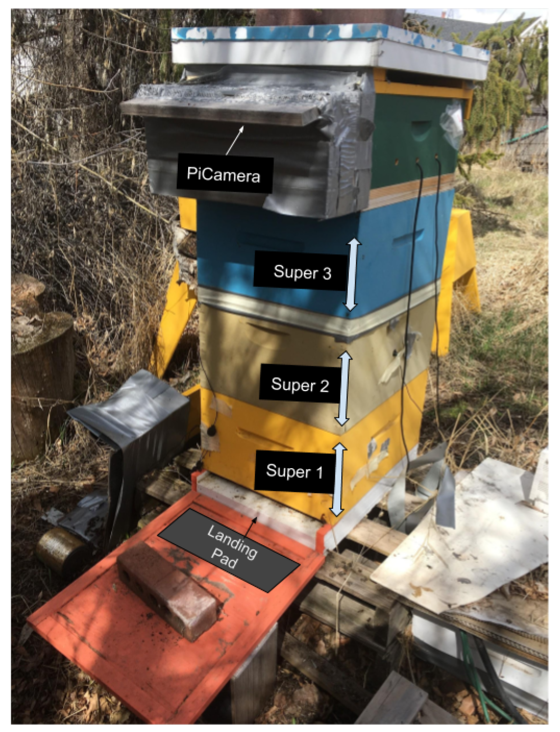
All video data for this investigation were captured by BeePi monitors, multi-sensor EBM systems we designed and built in 2014 [49], and have since been iteratively modifying [5,42,43,50,51]. Each BeePi monitor consists of a raspberry pi 3 model B v1.2 computer, a pi T-Cobbler, a breadboard, a waterproof DS18B20 temperature sensor, a pi v2 8-megapixel camera board, a v2.1 ChronoDot clock, and a Neewer 3.5 mm mini lapel microphone placed above the landing pad. All hardware components fit in a single Langstroth super (see Figure 1, Figure 2 and Figure 3). BeePi units operate either on the grid or on rechargeable batteries.

BeePi monitors have so far had five field deployments. The first deployment was in Logan, UT (September 2014) when a single BeePi monitor was placed into an empty hive and ran on solar power for two weeks. The second deployment was in Garland, UT (December 2014–January 2015), when a BeePi monitor was placed in a hive with overwintering honeybees and successfully operated for nine out of the fourteen days of deployment on solar power to capture ≈200 MB of data. The third deployment was in North Logan, UT (April 2016–November 2016) where four BeePi monitors were placed into four beehives at two small apiaries and captured ≈20 GB of data. The fourth deployment was in Logan and North Logan, UT (April 2017–September 2017), when four BeePi units were placed into four beehives at two small apiaries to collect ≈220 GB of audio, video, and temperature data [50]. The fifth deployment started in April 2018, when four BeePi monitors were placed into four beehives at an apiary in Logan, UT. This deployment is still ongoing, because in, September 2018, we made the decision to keep the monitors deployed through the winter to stress test the equipment in the harsh weather conditions of northern Utah. We have so far collected over 400 GB of video, audio, and temperature data. Data collection software is written in Python 2.7.9 [52].

2.2. Bee Motion Counting and Image Data

2.2.1. Bee Motion Counting

In this investigation, we focused on training and evaluating three types of classifiers— automatically and manually designed ConvNets, RFs, and linear SVMs—to classify motion regions. The curation of the image datasets, described in detail in the next two sections, is best construed in the context of the BeePi bee motion counting algorithm shown in Figure 4 and illustrated in the performance videos in the Supplementary Materials. Once mounted on top of a Langstroth beehive (see Figure 1), a BeePi monitor captures a 30-s video every 15 min from 8:00 to 21:00 at a resolution of 360 × 240 or 1920 × 1080 pixels. All frames from each captured video are processed for motion detection. We experimented with three motion detection algorithms available in OpenCV 3.0.0: KNN [38], MOG [39], and MOG2 [40]. Although all three algorithms performed on par, we experimentally found that MOG2 worked slightly better than either KNN or MOG, because it was less sensitive to shadows [51,53].

The output of the motion detection module is a set of image regions centered around detected motion points. We call these image regions motion regions. In Figure 4, the image with the subtitle “Motion Regions” shows detected motion regions as yellow squares. The yellow squares depict the cropped region boundaries around each detected motion point. The size of each square is a height-dependent parameter of the algorithm.

To understand how we chose the values of the height parameter, it is helpful to understand the basic beekeeping cycle in a Langstroth hive. Initially, after a beekeeper hives a fresh bee package in a Langstroth beehive, the hive consists of a single deep super (a rectangular wooden box 50.48 cm long, 41.28 cm wide and 24.45 cm high) with ten empty frames where the newly hived colony starts to develop. In a hive with a single deep super, a BeePi monitor is placed on top of that super. As the bees fill the frames in the first deep super with comb, pollen, and brood, the beekeeper places a second deep super with another ten frames on top of the first deep super to give the bee colony more space to expand and grow. After the second super is placed on top of the first one, the BeePi monitor is placed on top of the second super. While Langstoth hives with healthy colonies can potentially grow to be four or even five supers high, we confined the scope of this investigation to hives with one or two supers. We refer to the data captured from BeePi monitors on first supers as 1-super data and to the data captured from BeePi monitors on second supers as 2-super data. When the monitor is placed on a single super, the monitor’s camera is ≈35 cm above the hive’s landing pad and the camera’s field of view is ≈50 cm high and ≈80 cm wide. When the monitor is placed on the second super, the monitor’s camera is ≈60 cm above the landing pad and the camera’s field of view is ≈100 cm high and ≈160 cm wide.

When the BeePi monitor is placed on the first super (i.e., the camera is ≈35 cm above the landing pad), the size of each motion region is set to 150 × 150 pixels (see yellow squares in Figure 5). We experimentally found this size to be optimal in that, when cropped, 150 × 150 motion regions had a higher probability of containing at least one full-size bee than the other motion region sizes we tested. Specifically, to discover this size, we took samples of n × n motion regions from 1-super videos, where n ranged from 50 to 250 in increments of 10, and manually counted the percentage of samples containing at least one full-size bee for each sample size. The size of 150 × 150 had the highest percentage of regions with at least one full-size bee. When the monitor is placed on the second super (i.e., the camera is ≈60 cm above the landing pad), the size of each motion region is set to 90 × 90 pixels. This size was also experimentally found to be optimal in the same fashion as in the case of the single super in that 90 × 90 motion regions from 2-super videos contained the highest number of regions with at least one full-size bee.

Each detected motion region is classified by a trained classifier (e.g., a ConvNet, an RF, or an SVM) into two classes—BEE or NO-BEE. When a detected motion region is classified by a ConvNet, it is resized to fit the dimensions of the input layer of a particular ConvNet (i.e., 32 × 32 pixels or 64 × 64 pixels). In the case of an RF or an SVM, the size of each detected motion region is left unchanged. In Figure 4, two motion regions are shown under the title “Motion Region”. The upper region contains a bee while the bottom one does not. Similarly, in Figure 5, some motion regions contain bees or parts thereof while others do not. For each video, the BeePi video processing algorithm returns the number of omnidirectional bee motions within the camera’s field of view over a 30-s period. We call these numbers bee motion counts and use them as estimates of omnidirectional bee traffic levels.

Algorithm 1 outlines the pseudocode of our bee motion counting method described above. On Line 2, the video is segmented into frames. In each frame, all motions are detected on Line 3. On Lines 4–13, each motion point is boxed to become a motion region, resized when necessary, classified by a classifier, and the total bee motion count is increased if a bee is detected in the motion region. On Line 15, the count of detected bee motions is returned.

Algorithm 1CountBeeMotions (Video V, MotionDetector $MD$, Classifier $CL$, int H, and int W).

1: BeeMotionCount = 0; 2: For each frame F in V Do 3:  MotionPoints = Use $MD$ to detect motions in F; 4:  For each motion point P in MotionPoints Do 5:   MotionRegion = crop H x W box around P; 6:   If $CL$ is a ConvNet Then 7:    MotionRegion = Resize MotionRegion to the size of $CL$’s input layer 8:   End If 9:   CLR = Use $CL$ to classify Box; 10:   If CLR == BEE Then 11:    BeeMotionCount = BeeMotionCount + 1; 12:   End If 13:  End For 14: End For 15: Return BeeMotionCount;

2.2.2. BEE1 Dataset

The first dataset of 54,382 labeled images for this investigation, henceforth referred to as BEE1, was obtained from the videos captured by four BeePi monitors placed on four Langstroth hives with Italian honeybee colonies. Two monitors were deployed in an apiary in North Logan, UT, USA (${41.7694}^{\circ }$ N, ${111.8047}^{\circ }$ W) and the other two in an apiary in Logan, UT, USA (${41.7370}^{\circ }$ N, ${111.8338}^{\circ }$ W) from April 2017 to September 2017. The two apiaries were approximately 17 km apart. All four honeybee colonies were hived by the first author in late April 2017. We refer to the two hives with BeePi monitors in the first apiary (North Logan) as M${}_{17}^1$ and M${}_{17}^2$ and to the two hives with BeePi monitors in the second apiary (Logan) as M${}_{17}^3$ and M${}_{17}^4$. (The superscripts refer to monitor numbers; the subscripts refer to year 2017.) M${}_{17}^1$ and M${}_{17}^2$ were approximately 10 m apart with M${}_{17}^1$ facing west and M${}_{17}^2$ facing east. M${}_{17}^1$ was under a tree immediately to the north of it and received sunlight only from 15:00 to 18:30. M${}_{17}^2$ had no trees around it. M${}_{17}^3$ and M${}_{17}^4$ were completely under trees with only occasional sun rays penetrating the foliage.

Each video had a resolution of 360 × 240 with a frame rate of ≈25 frames per second. We randomly selected 40 videos from June 2017 and July 2017 and then sampled 400 frames from each video. Each selected frame was segmented into 32 × 32 images by randomly selecting the start and end coordinates of each region. This image segmentation process generated a total of 54,382 32 × 32 images. We used this image curation process, because, in 2017, motion detection was not yet integrated into the BeePi video analysis algorithm. Instead, a window-sliding approach was used on each frame.

We obtained the ground truth classification for BEE1 by manually labeling the 54,382 32 × 32 images with two categories—BEE (if it contained at least one bee) or NO-BEE (if it contained no bees or only a small part of a bee). The image dataset from the apiary in North Logan, UT (i.e., M${}_{17}^1$ and M${}_{17}^2$) was used for validation. The image dataset from the apiary in Logan, UT (i.e., from M${}_{17}^3$ and M${}_{17}^4$) was used for model training and testing. In BEE1, no differentiation was made between 1-super and 2-super images. Figure 6 shows a sample of images from BEE1. There were 19,082 BEE and 19,057 NO-BEE images randomly selected for training, 6362 BEE and 6362 NO-BEE images randomly selected for testing, and 1801 BEE and 1718 NO-BEE images randomly selected for validation.

We executed the MANOVA [54] analysis of BEE1 to determine whether its training (class 0), testing (class 1), and validation (class 2) images are statistically significantly different. We used the following image features as independent variables in our analysis: contrast [55], energy [56], and homogeneity [57]. The dependent variables were class 0, class 1, and class 2. The MANOVA analysis gave the Pillai coefficient of 0.018588, the F value of 107.47, and $Pr(>F)<2.2\times {10}^{-16}$. Since the p-value is <0.05, the training, testing and validation datasets of BEE1 are significantly different in terms of contrast, energy, and homogeneity.

We would like to note in passing that, while some publications that evaluate various data classification models split their data into training and testing datasets, we prefer to split our data into training, testing, and validation datasets that are statistically significantly different from each other according to the MANOVA analysis. This three-way splitting of the data lowers the chances of the training and testing datasets having a non-empty intersection with the validation dataset. The training and testing datasets are used for model training and testing (i.e., evaluation). The validation dataset is used exclusively for model selection. We also ensure that the data for the training and testing datasets and the data for the validation datasets come from different sources (i.e., different hives).

2.2.3. BEE2 Dataset

The second dataset of 112,879 labeled images for this investigation, henceforth referred to as BEE2, was obtained from the videos captured by four BeePi monitors on four Langstroth beehives with Carniolan honeybee colonies in Logan, UT, USA (${41.7370}^{\circ }$ N, ${111.8338}^{\circ }$ W) in May and June 2018. All colonies were hived in late April 2018 by the first author. We refer to the four hives with BeePi monitors as M${}_{18}^1$, M${}_{18}^2$, M${}_{18}^3$, and M${}_{18}^4$. (The superscripts denote monitor numbers; the subscripts refer to year 2018.) M${}_{18}^1$ and M${}_{18}^2$ were approximately 10 m apart with M${}_{18}^1$ facing south and M${}_{18}^2$ facing southwest. South-facing M${}_{18}^3$ was approximately 30 m north of M${}_{18}^1$ and M${}_{18}^2$. M${}_{18}^4$ was approximately 20 m west of M${}_{18}^3$ and faced south-west. M${}_{18}^1$ and M${}_{18}^2$ were completely under trees with only occasional sun rays penetrating the foliage. M${}_{18}^3$ was under the sun from 9:00 to approximately 13:00. M${}_{18}^4$ received direct sunlight from approximately 15:00 to 16:30.

A total of 5509 1-super videos and 5460 2-super videos were captured. All videos had a resolution of 1920 × 1080 pixels. The 1-super videos were captured from 5 May 2018 to the first week of June 2018, when the second supers were mounted on all four beehives and the BeePi monitors started capturing videos from the second deep supers. The 2-super videos were captured from the first week of June 2018 to the end of the first week of July 2018, when the third supers were mounted on all four beehives.

We randomly selected 50 1-super videos and another 50 2-super videos. The ground truth was obtained by using the MOG2 algorithm to automatically extract 58,201 150 × 150 detected motion regions from the 1-super videos and 54,678 90 × 90 detected motion regions from the 2-super videos. We manually labeled each region as BEE (if it contained at least one bee) or NO-BEE (if it contained no bees or only a small part of a bee). 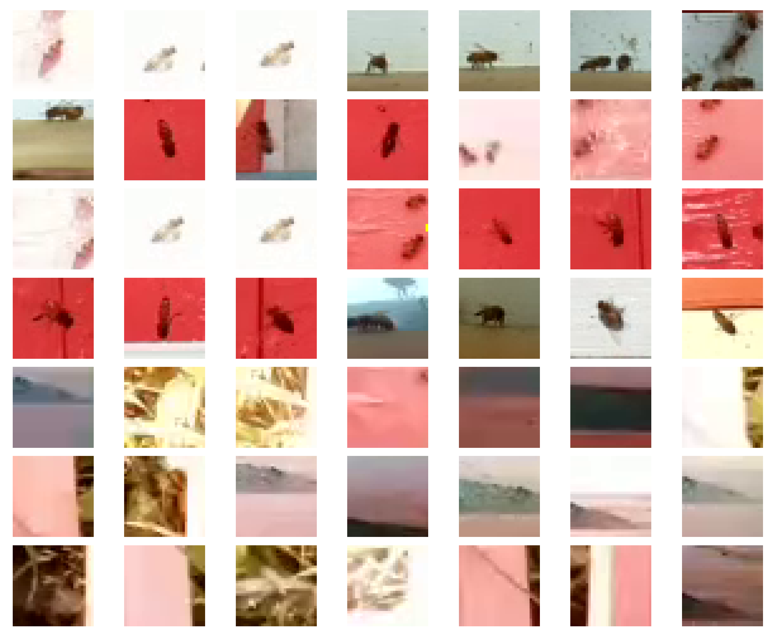Figure 7 and Figure 8 show samples of 1-super and 2-super images, respectively. We refer to the 1-super image dataset as BEE2_1S and to the 2-super image dataset as BEE2_2S.

Table 1. Numbers of images in BEE2_1S and BEE2_2S (collectively referred to as BEE2) used for training, testing, and validation.

	Train/Test (BEE)	Train/Test (NO-BEE)	Validate (BEE)	Validate (NO-BEE)	Total
BEE2_1S	11,094	36,143	8298	2666	58,201
BEE2_2S	17,176	21,310	6823	9369	54,678
Total	28,270	57,453	15,121	12,035	112,879

gives the exact numbers of labeled images in BEE2_1S and BEE2_2S used for training, testing, and validation. In both BEE2_1S and BEE2_2S, the images used for training and testing came from $M_{18}^1$ and $M_{18}^2$, while the validation images came from $M_{18}^3$ and $M_{18}^4$.

We executed the MANOVA [54] analyses of BEE2_1S and BEE2_2S to determine whether its training (class 0), testing (class 1), and validation (class 2) images are statistically significantly different. We used the following image features as independent variables: contrast [55], energy [56], and homogeneity [57]. The dependent variables were class 0, class 1, and class 2. For BEE2_1S, the MANOVA analysis gave the Pillai coefficient of 0.28849, the F value of 168.33, and $Pr(>F)<2.2\times {10}^{-16}$. For BEE2_2S, the MANOVA analysis gave the Pillai coefficient of 0.067891, the F value of 35.091, and $Pr(>F)<2.2\times {10}^{-16}$. Thus, since the p-value is <0.05 for both datasets, in both BEE2_1S and BEE2_2S, the training, testing, and validation images are significantly different from each other in terms of contrast, energy, and homogeneity.

2.3. Greedy Auto-Design of Convolutional Networks

A recent trend in the DL literature is the automation of designing DL architectures (e.g., [28,58]). The proponents of this approach argue that since successful DL models require considerable architecture engineering, it is worth it to automate DL model design for specific datasets. A disadvantage of this approach for low budget research projects or citizen scientist initiatives is the requirement of continuous access to considerable computational resources. For example, Baker et al. [58] used a Q-learning training procedure to develop constrained ConvNet architectures for a variety of image datasets on four GPUs for 8–10 days. Zoph et al. [28] used their Neural Architecture Search (NAS) framework to learn transferable DL architectures for CIFAR-10 and ImageNet on 500 GPUs over four days resulting in 2000 GPU-hours.

Since our research group had access to only one GPU for this investigation, we designed a multi-generational greedy grid search (GS) algorithm to automatically look for best-performing ConvNets by restricting the number of the DL architectural parameters and their value ranges and taking the hyperparameter values from the top N ConvNets, for different values of N given below, from the previous generation, where the generation number is the number of hidden layers (i.e., the number of convolutional and maxpooling layer pairs). Instead of exhaustively searching through each possible parameter value, as is done in standard grid search, our algorithm searches the space of ConvNet architectures constrained by the number of convolutional and maxpooling layer pairs (i.e., hidden layers), filter sizes, and the number of nodes in each hidden layer. An addition of a convolutional layer is always followed by an addition of a maxpooling layer with a kernel size of 2. All hidden layers use the ReLU activation function and the Adam optimizer [59]. The learning rate is set to 0.001; the loss function is the categorical cross-entropy that measures the probability error in classification tasks with mutually exclusive classes. Henceforth we refer to each ConvNet auto-designed through our greedy GS algorithm as ConvNetGS-x, where x denotes the number of hidden layers.

In searching the ConvNet architectures with one hidden layer, the number of nodes in the convolutional layer of the hidden layer varied from 1 to 32 and the filter size from 1 to 16. Algorithm 2 gives the pseudocode of our procedure for auto-designing ConvNets with a single hidden layer that consists of one convolutional layer followed by one maxpooling layer. On Line 3, an input layer of a specific size is created. On Lines 4–6, convolutional, maxpooling, and output layers are created. On Line 7, a ConvNet is created that consists of the input layer, the hidden layer (i.e., the convolutional layer followed by the maxpooling layer), and the output layer. The activation function in all layers of the newly created ConvNet is set to ReLU. The learning rate of the ConvNet is set to 0.001. The ConvNet’s optimizer function is set to adam. Each created ConvNet is then persisted on the disk. After the ConvNets are created and persisted on the disk, each of them is inflated from the disk, trained, evaluated, and persisted along with its validation performance, which is shown on Lines 13–15 in Algorithm 2.

Algorithm 2TrainGen1ConvNets (TrainSet TRS, TestSet TTS, ValidSet VST, and int NE).

1: For number of nodes $1\le N\le 32$ Do 2:  For filter size $1\le S\le 16$ Do 3:   IL = create input layer of size I × I, where I = 32 or I = 64; 4:   CL = create convolutional layer with N nodes and filter size S; 5:   ML = create maxpooling layer with kernel size 2; 6:   OL = create an output layer with two nodes: BEE and NO-BEE; 7:   NN1 = create a ConvNet that consists of IL, CL, ML, OL; 8:   Set NN1’s activation function to ReLU; 9:   Set NN1’s learning rate to 0.001; 10:   Set NN1’s optimizer function to adam; 11:   Persist NN1 on disk; 12:  End For 13:  Train and test each persisted NN1 on TRS and TTS for number of epochs given by NE; 14:  Validate each NN1 on VST; 15:  Perist NN1 and its validation results; 16: End For

In the ConvNet architectures with two hidden layers, for the first hidden layer, the numbers of hidden nodes and filter sizes were taken from the Top 15 best performing one-hidden-layer models. In the second hidden layer, the number of hidden nodes in the convolutional layer ranged from 34 to 65 and the filter size from 7 to 12. Algorithm 3 shows the pseudocode of our procedure for auto-designing ConvNets with two hidden layers. On Line 1, 15 top performing one-layer ConvNets are taken for a given validation dataset. In the outer for loop that starts on line 2, an input layer is created of a given size and the hidden layer’s architecture is taken from one of the top performing one-layer ConvNets. In the two nested for loops on Lines 5–14, two-layer ConvNets are created one by one. The architecture of the first hidden layer comes from a top performing single layer ConvNet. The parameters for the second hidden layer are defined by the specified ranges for the number of nodes and for the filter size. Each created ConvNet is persisted for later training, testing, and validation. On Lines 18–20, each newly created two-layer ConvNet is trained, tested, validated, and persisted with its trained weights and validation results.

Algorithm 3TrainGen2ConvNets (TrainSet TRS, TestSet TTS, ValidSet VST, and int NE).

1: NN1List = Take Top 15 best performing NN’s with 1 hidden layer; 2: For each NN1 in NN1List Do 3:  IL = create an input layer of size I × I, where I = 32 or I = 64; 4:  HL = take NN1’s hidden layer; 5:  For number of nodes $34\le N\le 65$ Do 6:   For filter size $7\le S\le 12$ Do 7:    CL2 = create convolution layer with N nodes and filter size S; 8:    ML2 = create a maxpooling layer with a kernel size 2; 9:    OL2 = create an output layer with 2 nodes: BEE and NO-BEE; 10:    NN2 = create a ConvNet that consists of IL, HL, CL2, ML2, OL2; 11:    Set NN2’s activation function to ReLU; 12:    Set NN2’s learning rate to 0.001; 13:    Set NN2’s optimizer function to adam; 14:    Persist NN2; 15:   End For 16:  End For 17: End For 18: Train and test each persisted NN2 on TRS and TST for number of epochs given by NE; 19: Validate NN2 on VST; 20: Perist NN2 and its validation results;

The algorithms for auto-designing deeper ConvNets are similar to Algorithms 1 and 2, and are not shown due to space considerations. In each deeper ConvNet with L hidden layers, the architectures of the previous $L-1$ layers are taken from the top N performing ConvNets with $L-1$ hidden layers. Thus, in the ConvNet architectures with three hidden layers, for the first and second hidden layers, the numbers of hidden nodes and filter sizes were taken from the Top 15 best performing two-hidden-layer models. For the third layer, the number of nodes in the convolutional layer ranged from 65 to 130 and the filter size from 7 to 12. In the ConvNet architectures with four hidden layers, for the first, second and third hidden layers, the numbers of hidden nodes and filter sizes were taken from the Top 10 best performing three-hidden-layer models. The number of hidden nodes in the fourth layer ranged from 120 to 300 and the filter size from 7 to 12. In the ConvNet architectures with five hidden layers, for the first, second, third and fourth hidden layers, the numbers of hidden nodes and filter sizes were taken from the Top 10 best performing four-hidden-layer models. The number of hidden nodes in the fifth layer ranged from 240 to 650 and the filter size from 7 to 12. In the ConvNet architectures with six hidden layers, for the first, second, third, fourth, and fifth hidden layers, the numbers of hidden nodes and filter sizes ranged from the Top 5 best performing five-hidden-layer models. The number of hidden nodes in the sixth layer ranged from 600 to 1240 and the filter size from 7 to 12.

3. Experiments and Results

3.1. Experiments with BEE1

In the first set of our experiments, we focused on our auto-designed ConvNets. The actual training, testing, and validation procedures were implemented in Python 3.4 with tflearn [60] and executed on an Ubuntu 16.04.S LTS computer with an AMD Ryzen 7 1700X Eight-Core Processor with 16 GiB of DDR4 RAM and a GeForce GTX 1080 Ti GPU with 11 GB of onboard memory. Each model was trained for 50 epochs with a batch size of 50. Each image was normalized to have the pixel values on each channel to be in the range [0, 1].

Table 2. Performance of best auto-designed ConvNet models on BEE1. Each network was trained for 50 epochs. The number following the model type (ConvNetGS—GS stands for greedy search) shows the number of hidden layers in each ConvNet. A hidden layer consists of a convolutional layer followed by a maxpooling layer. The validation accuracies are sorted from highest to lowest. The architecture of ConvNetGS-3 is given in Figure A1 in Appendix A.

Model	BEE Acc.	NO-BEE Acc.	Valid Accuracy
ConvNetGS-3	98.48%	99.66%	99.09%
ConvNetGS-5	98.37%	99.66%	99.03%
ConvNetGS-2	98.25%	99.06%	98.66%
ConvNetGS-4	97.72%	99.50%	98.63%
ConvNetGS-1	98.71%	0.88%	48.52%

gives a performance summary of the best auto-designed ConvNets with the number of hidden layers in the range [1, 5] on the validation dataset of BEE1. The best one-hidden-layer model had a filter size of 9, 29 hidden nodes, and a validation accuracy of 48.52%. The best performing two-hidden-layer model had 31 nodes with a filter size of 12 in the first hidden layer and 40 notes with a filter size of 10 in the second hidden layer. This model had a validation accuracy of 98.66%. The best performing three-hidden-layer model had 27 hidden nodes in Layer 1 with a filter size of 9, 42 hidden nodes in Layer 2 with a filter size of 11, 105 hidden nodes with a filter size of 11 in Layer 3, and a validation accuracy of 99.09%. The best performing four-hidden-layer model had 27 hidden nodes with a filter size of 9 in layer 1, 38 hidden nodes with a filter size of 9 in Layer 2, 85 hidden nodes with a filter size of 9 in Layer 3, 220 hidden nodes with a filter size of 10 in Layer 4, and a validation accuracy of 98.63%. The best performing five-hidden-layer model had 27 hidden nodes with a filter size of 9 in layer 1, 38 nodes with a filter size of 9 in Layer 2, 85 nodes with a filter size of 9 in Layer 3, 260 nodes with a filter size of 8 in Layer 4, 240 nodes with a filter size of 9 in Layer 5, a testing loss of 0.03, and a validation accuracy of 99.03%.

In the ConvNet architectures with six hidden layers (not shown in Table 2), for the first, second, third, fourth, and fifth hidden layers, the numbers of hidden nodes and filter sizes ranged from the Top 5 best performing five-hidden-layer ConvNets. The number of hidden nodes in Layer 6 ranged from 600 to 1240 and the filter size from 7 to 12. The best performing six-hidden-layer model had 27 hidden nodes with a filter size of 9 in layer 1, 38 nodes with a filter size of 9 in Layer 2, 85 nodes with a filter size of 9 in Layer 3, 260 nodes with a filter size of 8 in Layer 4, 240 nodes with a filter size of 9 in Layer 5, 1160 nodes with a filter size of 9 in Layer 5, and a validation accuracy of 99.03%, which was not better than the performance results of ConvNetGS-5 from the previous generation. Adding more hidden layers (seven and eight) did not improve the validation performance of the auto-designed ConvNets in that the average validation accuracy varied from 98.90% to 99.09%.

We next compared the performance of our auto-designed ConvNets with hand-designed ConvNets on the same dataset. Toward that end, we organized a deep learning competition on BEE1. The competition was organized as a longitudinal class project in a graduate Computer Science course taught by the first author at Utah State University in Fall 2018. There were 52 graduate and upper-level undergraduate students enrolled in this course. The students received detailed instruction on the best ConvNet design practices [12,29,61,62] and the ConvNet design and training tools (e.g., tflearn [60] and TensorFlow [63]) and were asked to design, train, and test ConvNets on the training and testing images of BEE1. Each ConvNet was evaluated on the validation dataset of BEE1, which was withheld from the students during the design, training, and testing phases. Only the networks with a validation accuracy of 97% or above were chosen, which gave us nine ConvNets.

The architecture of the best performing hand-designed ConvNet (ConvNet 1) with a validation accuracy of 99.45% is given in Figure 9. In addition to the input and output layers, this ConvNet has six hidden layers. Specifically, it consists of three convolutional layers, each of which is followed by a maxpooling layer. Each convolutional layer doubles the number of filters in the convolutional layer: the first convolutional layer has 64 3 × 3 filters, the second one 128 3 × 3 filters, and the third one 256 3 × 3 filters. All convolutional layers have the ReLU activation function and a weight decay of 0.001. The convolutional and maxpooling layers are followed by four FC layers of 512 units, 256 units, 128 units, and 64 units. Each of these layers has the ReLU activation function and a dropout of 0.5. The last FC layer has the softmax activation function, the adam optimizer, a learning rate of 0.0001, and the categorical cross entropy as its loss function.

To obtain the standard machine learning (ML) benchmarks, we trained and validated RFs and SVMs on BEE1. Each image was normalized and flattened so that the inputs to the SVMs and RFs were the same as the inputs to the ConvNets. We varied the number of trees in RFs from 20 to 100 in increments of 20. All RFs were trained with the gini entropy function. The minimum number of samples required to split and the minimum number of samples required to be at a leaf node were both set to 2. The best performing RF on the validation dataset of BEE1 (see

Table 3. Performance of top hand-designed ConvNet, ResNet32, and VGG16 models (trained for 100 epochs), RFs, and SVMs on BEE1. The number following the RF abbreviation denotes the number of trees. The two top performing auto-designed ConvNets on BEE1 (ConvNetGS-3 and ConvNetGS-5) are included for comparison. The validation accuracies are sorted from highest to lowest.

Model	BEE Acc.	NO-BEE Acc.	Valid Accuracy
ConvNet 1	99.06%	99.89%	99.48%
ResNet32	99.12%	99.83%	99.48%
ConvNetGS-3	98.48%	99.66%	99.09%
ConvNet 2	99.07%	99.12%	99.09%
ConvNetGS-5	98.37%	99.66%	99.03%
ConvNet 3	99.07%	98.95%	99.01%
VGG16	97.90%	99.83%	98.87%
ConvNet 4	98.95%	98.78%	98.87%
ConvNet 5	98.37%	99.17%	98.77%
ConvNet 6	98.60%	98.84%	98.72%
ConvNet 7	97.96%	98.28%	98.13%
ConvNet 8	98.43%	96.19%	97.31%
ConvNet 9	97.67%	96.85%	97.26%
RF (40)	90.55%	96.80%	93.67%
RF (80)	90.88%	96.10%	93.49%
RF (100)	90.33%	96.16%	93.24%
RF (20)	89.89%	96.16%	93.02%
RF (60)	89.89%	95.98%	92.94%
SVM	58.29%	69.03%	63.66%

) was the RF with 40 trees whose accuracy was 93.67%. All SVMs used the linear kernel with the max-iter parameter varying from 10 to 1000, an L2 penalty, a squared hinge loss function, and a tolerance of 0.0001. The best accuracy of 63.66% on the validation dataset was achieved by the linear SVM with a max-iter of 1000. For more thorough comparison, we also trained, tested, and validated ResNet32 [64] and VGG16 [14], two popular ConvNet architectures frequently referenced in the DL literature on image classification. We did not use any pre-trained weights in ResNet32 or VGG16. Both ConvNets were trained from scratch with no internal layer optimization.

Table 3 summarizes the performance results of the ConvNets, RFs, and SVMs and compares them with the results of the two top performing auto-designed ConvNets (ConvNetGS-3 and ConvNetGS-5) on BEE1. The results in Table 2 and Table 3 show that, on BEE1, ResNet32 and ConvNet 1 tied for first place with a validation accuracy of 99.48%. The best auto-designed ConvNet (ConvNetGS-3) came a close second with a validation accuracy of 99.09%. Thus, the top two ConvNets performed only slightly better than the top performing auto-designed ConvNet. ConvNetGS-3 tied for the second place with ConvNet 2 and outperformed all other ConvNets, VGG16, RFs, and SVMs. The RFs performed much better than the linear kernel SVMs but were ≈6% below the best hand- and auto-designed ConvNets.

3.2. Experiments with BEE2

To transfer the representations learned on BEE1 over to BEE2, we started our experiments on BEE2 with the ConvNets automatically designed with greedy grid search on BEE1. Specifically, we took the five ConvNetGS models (see Table 2) and trained and validated them on BEE2_1S and BEE2_2S (see Table 1). Each ConvNetGS was trained for 50 epochs.

Table 4. Performance of five auto-designed ConvNets on BEE2_1S validation dataset. Each ConvNet was trained for 50 epochs. The number in the first column following the abbreviation ConvNetGS specifies the number of hidden layers; validation accuracies are sorted from highest to lowest. The architecture of ConvNetGS-4 is given in Figure A2 in Appendix A.

Model	BEE Acc.	NO-BEE Acc.	Overall Acc.
ConvNetGS-4	84.86%	91.03%	86.36%
ConvNetGS-3	82.18%	90.73%	84.26%
ConvNetGS-1	82.09%	80.23%	81.63%
ConvNetGS-5	76.37%	95.76%	81.09%
ConvNetGS-2	76.21%	95.04%	80.79%

and

Table 5. Performance of five auto-designed ConvNets on BEE2_2S validation dataset. Each ConvNet was trained for 50 epochs. The number in the first column following the abbreviation ConvNetGS specifies the number of hidden layers. The validation accuracies are sorted from highest to lowest. The architecture of ConvNetGS-5 is given in Figure A3 in Appendix A.

Model	BEE Acc.	NO-BEE Acc.	Overall Acc.
ConvNetGS-5	74.52%	77.42%	76.20%
ConvNetGS-4	64.82%	83.39%	75.56%
ConvNetGS-3	64.94%	79.93%	73.61%
ConvNetGS-2	65.70%	76.77%	72.10%
ConvNetGS-1	66.04%	68.36%	67.38%

summarize the performance results of these auto-designed ConvNets on both validation datasets.

We took the Top 9 performing hand-designed ConvNets from BEE1 (see Table 3) and trained and validated them on both BEE2_1S and BEE2_2S. We also trained, tested, and validated ResNet32 [64] and VGG16 [14] on these datasets. To obtain the standard ML benchmarks, we again trained, tested, and validated on BEE2_1S and BEE2_2S the same linear SVMs and RFs that we trained, tested, and validated on BEE1. Each image was normalized and flattened so that the inputs to the SVMs and RFs were the same as the inputs to the ConvNets.

Table 6. Model performance on BEE2_1S validation dataset; all hand-designed ConvNets, ResNet32, and VGG16 were trained for 100 epochs each. The two top performing auto-designed ConvNets (ConvNetGS-4 and ConvNetGS-3) are included for comparison. The overall accuracy is sorted from highest to lowest.

Model	BEE Acc.	NO-BEE Acc.	Overall Acc.
ConvNet 1	94.34%	93.24%	94.08%
ConvNet 3	88.44%	88.44%	88.84%
VGG16	78.09%	95.12%	86.60%
ConvNetGS-4	84.86%	91.03%	86.36%
ConvNetGS-3	82.18%	90.73%	84.26%
ConvNet 7	81.64%	88.85%	83.39%
ConvNet 6	72.02%	86.45%	75.53%
ConvNet 2	67.99%	93.66%	74.82%
RF (100)	50.27%	98.31%	74.29%
RF (60)	50.07%	98.34%	74.21%
RF (80)	49.90%	97.86%	73.88%
RF (40)	49.53%	97.82%	73.67%
ConvNet 4	66.48%	95.87%	73.44%
RF (20)	46.62%	97.26%	71.94%
SVM	87.66%	51.06%	69.36%
ResNet-32	38.11%	99.70%	68.90%
ConvNet 9	60.49%	89.42%	67.53%
ConvNet 5	0%	100%	24.31%
ConvNet 8	0%	100%	24.31%

and

Table 7. Model performance on BEE2_2S validation dataset; all ConvNets, ResNet32, and VGG16 were trained for 100 epochs each. The two top performing auto-designed ConvNets (ConvNetGS-5 and ConvNetGS-4) are included for comparison. The overall accuracy is sorted from highest to lowest.

Model	BEE Acc.	NO-BEE Acc.	Overall Acc.
ConvNet 3	75.59%	81.31%	78.90%
ConvNet 1	69.98%	94.84%	78.17%
ConvNet 4	65.73%	84.36%	76.51%
ConvNetGS-5	74.52%	77.42%	76.20%
ConvNet 2	64.34%	90.51%	75.92%
ConvNetGS-4	64.82%	83.39%	75.56%
ConvNet 5	57.37%	90.06%	73.77%
ResNet32	64.10%	83.37%	73.73%
ConvNet 9	52.04%	87.49%	72.55%
VGG16	60.78%	82.54%	71.66%
ConvNet 6	51.77%	86.04%	68.90%
SVM	87.10%	41.95%	64.53%
RF (60)	39.05%	88.99%	64.02%
RF (80)	37.84%	88.34%	63.09%
RF (100)	37.71%	88.43%	63.07%
RF (40)	37.34%	87.83%	62.58%
RF (20)	35.36%	89.89%	62.62%
ConvNet 7	0%	100%	57.86%
ConvNet 8	0%	100%	57.86%

give the performance results of the hand-designed ConvNets, ResNet32, VGG16, the two top ConvNetGS models, and the ML models on BEE2_1S and BEE2_2S, respectively. In both tables, the parenthesized numbers following the RF abbreviation specify numbers of trees. The architecture of the best performing hand-designed ConvNet for BEE2_1S (ConvNet 1) is the same as the architecture of the best performing ConvNet for BEE1 (see Figure 9), except the input layer is 64 × 64, as shown in Figure 10. The architecture of the best performing hand-designed ConvNet on BEE2_2S (ConvNet 3) is shown in Figure 11. On BEE2_1S, ConvNetGS-4 was the best-performing auto-designed model; on BEE2_2S, it was outperformed by ConvNetGS-5.

As shown in Table 6, on BEE2_1S, the two hand-designed ConvNets (ConvNets 1, 3) outperformed all other models, including ResNet32 and VGG16. The two top performing auto-designed ConvNets (ConvNetGS-4 and ConvNetGS-3) ranked fourth and fifth, respectively. The performance of the auto-designed ConvNets was better than the performance of the other seven hand-designed ConvNets, ResNet32, the RFs and the SVMs. The performance of the random forests improved on BEE2_1S. In particular, the RF with 100 trees outperformed four hand-designed ConvNets, ResNet32, and the best linear kernel SVM by significant margins.

As shown in Table 7, on BEE2_2S, hand-designed ConvNets 3, 1, and 4 performed better than the two auto-designed ConvNets and took the Top 3 slots. The top performing auto-designed ConvNets, ConvNetGS-5 and ConvNetGS-4, ranked fourth and seventh, respectively. It is interesting to note that the auto-designed ConvNets outperformed both ResNet32 and VGG16. The best linear SVM model slightly outperformed the best RF with 60 trees and ranked much higher than on BEE1 or BEE2_1S.

4. Preliminary Evaluation on Omnidirectional Bee Traffic Videos

We made a preliminary, proof-of-concept evaluation of the system’s performance on four omnidirectional bee traffic videos with different levels of bee traffic. We took random samples of 30-s timestamped videos from the validation beehives (i.e., the hives from which we acquired the validation images for BEE2_1S and BEE2_2S) to ensure that there was no overlap with the videos from which the training and testing images were obtained. In particular, we took a random sample of 30 videos from the early morning period (06:00–08:00), a random sample of 30 videos from the early afternoon period (13:00–15:00), a random sample of 30 videos from the late afternoon (16:00–18:00), and a random sample of 30 videos from the evening videos (19:00–21:00). All videos were captured in June and July, 2018. We chose these time periods to ensure that we have videos with different levels of omnidirectional bee traffic. According to our beekeeping experience in Logan and North Logan, Utah, in June and July, there is no or low bee traffic early in the morning or late in the evening and higher bee traffic in the afternoon when foragers leave for and return with nectar, pollen, and water.

We then randomly chose one video from each sample of 30 videos to obtain one video for each time period. The Supplementary Materials include the four videos and their textual descriptions. We then counted full bee motions, frame by frame, in each video. The number of bee motions in the first frame of each video (Frame 1) was taken to be 0. In each subsequent frame, we counted the number of full bees that made any motion when compared to their positions in the previous frame. A full bee was considered to have made a motion if it was not in a previous frame but appeared in the following frame (e.g., when it flew into the camera’s field of view). The Supplementary Materials include four CSV files with frame-by-frame full bee motion counts. The four videos were arbitrarily classified on the basis of the human bee motion counts as no traffic (NT) (NT_Vid.mp4), low traffic (LT) (LT_Vid.mp4), medium traffic (MT) (MT_Vid.mp4), and high traffic (HT) (HT_Vid.mp4). It took us approximately 2 h to count bee motions in NT_Vid.mp4, 4 h in LT_Vid.mp4, 5.5 h in MT_Vid.mp4, and 6.5 h in HT_Vid.mp4, for a total of 18 h for all four videos.

We ran our system on each of the four videos. In each video, motion detection was done with MOG2 [40] while motion region classification was done with VGG16, ResNet32, ConvNetGS3, and ConvNetGS4. The Supplementary Materials include the performance videos for each configuration of the system (i.e., MOG2/VGG16, MOG2/ResNet32, MOG2/ConvNetGS3, MOG2/ConvNetGS4). Each video shows the real-time performance of the system on a specific video so that the green rectangle regions show detected motion regions classified as BEE and the blue rectangle regions show detected motion regions classified as NO-BEE. Given a video, the system returns the total number of bee motions detected in it (see Algorithm 1 in Section 2.2.1).

Table 8. Performance of the system on the four evaluation videos NT_Vid.mp4, LT_Vid.mp4, MT_Vid.mp4, and HT_Vid.mp4: the columns VGG16, ResNet32, ConvNetGS3, and ConvNetGS4 give the bee motion counts returned by the configurations MOG2/VGG16, MOG2/ResNet32, MOG2/ConvNetGS3, and MOG2/ConvNetGS4, respectively; the last column gives the human bee motion counts for each video.

Video	Num. Frames	VGG16	ResNet32	ConvNetGS3	ConvNetGS4	Human Count
NT_Vid.mp4	742	151	75	182	127	73
LT_Vid.mp4	744	47	25	57	43	353
MT_Vid.mp4	743	1245	145	597	316	2924
HT_Vid.mp4	744	16,647	13,362	16,569	15,109	5738

gives the bee motion counts returned by each configuration of the system and the human bee motion counts. For NT_Vid.mp4, where there is only one bee flying into a hive, the human bee count is 73 full bee motions, which is closely approximated by the MOG2/ResNet32 configuration. The other configurations roughly double the human bee motion count. When a bee is flying, the motion detection algorithm (e.g., MOG2) sometimes detects motion centered on several bee body parts (e.g., a thorax or a wing). In this case, the motion regions necessarily intersect on the same bee, in which case the motion region classifier (e.g., VGG16) is likely to classify some of the intersecting motion regions as BEE, which increases the bee motion counts. This overlapping classification can be observed in all the performance videos given in the Supplementary Materials.

The second most common cause of bee motion count overestimation was false positives, especially shadows. In many movies captured by BeePi monitors on sunny days, shadows either closely follow moving bees or reflect bees that are not even in the camera’s field of view. Figure 12 gives several motion regions that were classified as BEE by all convolutional neural networks. In attempting to explain this behavior, we concluded that the training datasets had insufficient numbers of bee shadow images in the NO-BEE category. This is the most likely explanation why the networks had a tendency to classify many bee shadows as BEE.

As shown in Table 8, in the case of the low traffic video, LT_mid.mp4, all four configurations underestimated the numbers of full bee motions. All four bee motion counts are less than 100, whereas the human bee motion count equals 353. A visual analysis of the four performance videos for this video included in the Supplementary Materials reveals that not all bee motion regions are detected. For example, if a bee is flying quickly, only a couple of bee motions may be detected and classified as a bee. In the case of the medium traffic video, MT_vid.mp4, all four configurations also underestimated the numbers of full bee motions. The MOG2/VGG16 configuration came closest to the human bee motion count while the other three configurations significantly underestimated it. The four performance videos for MT_vid.mp4 (see the Supplementary Materials) indicate that not all bee motion regions were detected in the medium traffic video. Hence, the underestimation of the human count by all four system configurations. For the high traffic video, HT_mid.mp4, all four configurations overestimated the human count of full bee motions. The performance videos for HT_mid.mp4 in the Supplementary Materials show that all ConvNets misclassified many motion regions with grass blade or leaf motions as BEE.

In a preliminary test of whether the system can distinguish among different levels of omnidirectional bee traffic, we randomly selected another four videos from the same four time periods: early morning, early afternoon, late afternoon, and late evening. These four videos (NT_Vid02.mp4, LT_Vid02.mp4, MT_Vid02.mp4, HT_Vid02.mp4) are also included in the Supplementary Materials. We did not obtain human bee motion counts for these videos. Rather, we watched each video and qualitatively classified it as no traffic (NT), low traffic (LT), medium traffic (MT), or high traffic (HT).

Table 9. Performance of the system on NT_Vid02.mp4, LT_Vid02.mp4, MT_Vid02.mp4, and HT_Vid02.mp4: the columns VGG16, ResNet32, ConvNetGS3, and ConvNetGS4 give the bee motion counts returned by the configurations MOG2/VGG16, MOG2/ResNet32, MOG2/ConvNetGS3, and MOG2/ConvNetGS4, respectively.

Video	Num. Frames	VGG16	ResNet32	ConvNetGS3	ConvNetGS4
NT_Vid02.mp4	743	140	188	175	173
LT_Vid02.mp4	744	530	1101	1439	10,000
MT_Vid02.mp4	743	1095	343	1179	871
HT_Vid02.mp4	744	13,002	9716	9960	9885

gives the bee motion counts of the four configuration for each video. The results indicate that the MOG2/VGG16 configuration distinguishes among NT, LT, MT, and HT in terms of bee motion counts. The other three configurations are not as consistent. In LT_Vid02.mp4 and MT_Vid02.mp4, the three ConvNets classify as BEE regions with grass blade or leaf motions or regions with leaf motions that contain dead bees.

5. Discussion

Our experiments indicate that the proposed two-tier method of coupling motion detection with image classification to count bee motions in close proximity to the landing pad of a given hive has the potential to improve estimates of omnidirectional bee traffic levels in EBM. In the proposed method, motion detection acts as a class-agnostic object location method to suggest regions with possible objects, each of which is subsequently classified with a trained classier such as a ConvNet or an SVM or an ensemble of classifiers such as an RF.

In our experiments, the hand-designed ConvNets performed slightly better than or on par with the auto-designed ConvNets on two of the three image datasets (BEE1 and BEE2_1S). When the hand-designed ConvNets outperformed the auto-designed ConvNets, the performance margins were not wide. Specifically, on BEE1 (see Table 2 and Table 3), the best hand-designed ConvNet (ConvNet 1) and ResNet32 achieved a validation accuracy of 99.48% while the performance of the best auto-designed ConvNet (ConvNetGS-3) was 99.09%. Thus, the best auto-designed ConvNet performed almost exactly on par with the best hand-designed ConvNet and ResNet32 and outperformed the remaining seven hand-designed ConvNets, VGG16, and all RFs and SVMs. The performance margin between the best hand-designed ConvNet (ConvNet 1) and the best auto-designed ConvNet (ConvNetGS-3) was only 0.39%.

On BEE2_1S (see Table 4 and Table 6), the top two hand-designed ConvNets (ConvNets 1 and 3) outperformed all other models with the respective validation accuracies of 94.08% and 88.84%. The two best performing auto-designed ConvNets (ConvNetGS-4 and ConvNetGS-3) ranked fourth and fifth with the respective validation accuracies of 86.36% and 84.26%. Thus, the auto-designed ConvNets outperformed the remaining seven hand-designed ConvNets, ResNet32, and all RFs and SVMs. The performance margin between the best hand-designed ConvNet (ConvNet 1) and the best auto-designed ConvNet (ConvNetGS-4) was 7.7%.

On BEE2_2S (see Table 5 and Table 7), the top three places were taken by hand-designed ConvNets (ConvNets 3, 1, and 4). These ConvNets outperformed the other models with the respective validation accuracies of 78.90%, 78.17%, and 76.51%. The top auto-designed model (ConvNetGS-5) ranked fourth with a validation accuracy of 76.20% and outperformed both ResNet32 and VGG16. The performance margin between the best performing hand-designed ConvNet and the best performing auto-designed ConvNet narrowed to 2.7%.

A solid performance of the RFs on BEE1 and BEE2_1S is noteworthy. Typically, RFs do well on datasets of items structured as sets of features [37]. However, in our experiments, we trained and validated the RFs on raw images without extracting any features. Each pixel position and its corresponding value can, of course, be construed as a feature-value pair, but this does not require any computationally intensive feature extraction typically done for classifiers that use feature-value pairs. While the RFs did not outperform any hand- or auto-designed ConvNets on BEE1, the validation accuracy of all RFs was above 90%. On BEE2_1S, the top performing RF with 100 decision trees performed better than four hand-designed ConvNets, ResNet32, and the best linear SVM. Our experiments suggest that a more principled automation of RF designs for specific image datasets may yield classifiers whose performance approaches the performance of hand- or auto-designed ConvNets. An advantage of RFs for EBM projects or for other low budget research projects and citizen science initiatives is that their training and validation is much faster than the training and validation of ConvNets or SVMs and does not require continuous access to large GPU farms. For example, it took us a total of 917.52 GPU hours (38.23 days) to finish training, testing, and validating all ConvNets with greedy GS and another 360.25 GPU hours (15 days) to train, test, and validate all hand-designed ConvNets, ResNet32, and VGG16. By way of comparison, training, testing, and validating all RFs on the same GPU computer took only ≈15 h.

Another observation we made is that our hand- and auto-designed ConvNets appear to have performed mostly on par with ResNet32 or VGG16, which suggests that all training and validation of DL models is local. ConvNet architectures that do well on large generic datasets are not guaranteed to do well on more specialized datasets. The overall performance of all classifiers on BEE1 was better than their overall performance on BEE2. A visual comparison of BEE1 and BEE2 datasets shows that BEE1 appears to be more homogenous in that the images in the training, testing, and validation datasets, while statistically significantly different in terms of contrast, energy, and homogeneity, appear to be more qualitatively similar to each other than the images in the training, testing, and validation datasets of BEE2. Another qualitative difference between BEE1 and BEE2 is that the validation dataset of BEE2 contains many more images of bee shadows than the validation dataset of BEE1. The image size of BEE1 (32 × 32) is smaller than the image size of BEE2 (64 × 64), which indicates that ConvNets, random forests, and SVMs may generalize better on smaller images than on larger ones.

Our evaluation of the proposed method on bee traffic videos is only preliminary. Hence, our observations should be interpreted with caution. Nonetheless, they provide valuable insights into how bee motion counts can be used in estimating omnidirectional bee traffic levels. These insights will inform our future work on video analysis of bee traffic. In some cases, the proposed method overestimated the human bee motion counts. Our analysis of the performance videos (see the Supplementary Materials) showed that a major cause of overestimation was overlapping motion regions. When several motion points were detected around a single bee, the motion regions cropped around them included the same bee whose motion was counted several times. This limitation can be met by obtaining estimates of overlap and counting motion regions with significant overlap as one motion region. Another cause of overestimation was false positives when the second tier of the proposed bee motion counting method misclassified motion regions containing bee shadows, grass blades or leaves as bees. One way to address false positives is to make training and testing datasets more representative by adding to them more samples of bee shadows, grass blades, and leaves.

In some cases, the proposed method underestimated the human bee motion counts. This underestimation appears to have been caused by false negatives, when second tier classifiers failed to recognize bees, as well as motion detection failures when the first tier motion detectors failed to detect motion altogether. The latter was observed with fast flying bees. We plan to experiment with higher video resolutions to estimate whether they can help us capture fast motions more accurately.

When we ran our system on the four videos with different levels of bee traffic, for which we did not obtain human counts, we discovered that some motion detection and classification configurations (e.g., MOG2/VGG16) could distinguish no traffic, low traffic, medium traffic and high traffic in terms of bee motion counts. This observation, while obviously preliminary, raises an important question of how accurately bee motion counts obtained by the proposed method should approximate the human bee motion counts. In some sense, the closeness of approximation may be irrelevant so long as automatically obtained bee motion counts enable the system to distinguish different bee traffic levels in order to track omnidirectional bee traffic over time. More experiments are obviously needed to validate this conjecture. The necessity to conduct more experiments leads to another important question of what ground truth videos are needed and how they should be obtained. The fact that it took us ≈18 h to obtain human bee motion counts on four videos of live bee traffic indicates that obtaining the ground truth in this manner is very labor intensive. A less expensive approach may be to obtain qualitative human classifications of bee traffic videos as no traffic, low traffic, medium traffic, and high traffic and then to seek ranges of automatic bee motion counts that enable the system to reliably distinguish different bee traffic levels.

Our current beekeeper logs capture such variables as drawn comb, liquid honey, eggs, pollen, larvae, capped brood, capped honey, drone brood, and comb. In the future, we plan to add bee traffic estimates to our logs. While accurate visual evaluations of bee traffic levels when bee traffic is very high are difficult and time-consuming, they may provide solid ground truth for videos with low or medium bee traffic levels.

To approximate human beekeepers’ assessments of bee colony health, future EBM monitors will need robust models capable of correlating digital interpretations of captured sensor data with human beekeeper observations. When such correlations become reasonably accurate, EBM monitors will be able to make more accurate assessments of bee colony health or of environmental states. An important knowledge engineering task ahead is the formalization of human beekeeper observations so that they can be correlated in a meaningful way with digital observations. It remains to be seen whether such formalizations can be generated by computer vision from field pictures of hive frames.

6. Conclusions

In this investigation, we proposed, implemented, and partially evaluated a two-tier method for counting bee motions in video analysis of omnidirectional bee traffic. Our method couples motion detection with image classification so that motion detection acts as a class-agnostic object location method that generates a set of regions with possible objects and each such region is classified by a class-specific classifier or an ensemble of classifiers such as a random forest. The method has been, and is being field tested in multiple BeePi monitors, our multi-sensor EBM systems. Our evaluation of several DL and ML models on three large image datasets obtained from the data captured by different BeePi monitors indicates that image classification can be added to a repertoire of EBM algorithms. In our future work, we plan to work on correlating omnidirectional bee motion counts with ambient temperature readings and formalized human beekeeper observations. To ensure the replicability of the reported findings and to provide a performance benchmark for interested research communities and citizen science initiatives, we have made public our curated image datasets, BEE1 (54,382 images) and BEE2 (112,879 images), used in this investigation. The Supplementary Materials include four bee traffic videos with corresponding human motion counts, sixteen performance videos that illustrate how different system configurations process bee traffic videos, and four bee traffic videos with no human motion counts which we used to estimate if the proposed system can distinguish among different bee traffic levels.