Article

Pressure Observer Based Adaptive Dynamic Surface Control of Pneumatic Actuator with Long Transmission Lines

1
School of Mechatronic Engineering, China University of Mining and Technology, Xuzhou 221116, China
2
National Quality Supervision and Inspection Centre of Pneumatic Products, Ningbo 315500, China
*
Author to whom correspondence should be addressed.
Appl. Sci. 2019, 9(17), 3621; https://doi.org/10.3390/app9173621
Submission received: 22 July 2019 / Revised: 24 August 2019 / Accepted: 26 August 2019 / Published: 3 September 2019
(This article belongs to the Special Issue Engineering for Surgery)

Abstract

:

Featured Application

This research dedicates to develop a pressure observer based nonlinear controller for precise position control of the MRI-compatible pneumatic servo system with long transmission lines.

Abstract

In this paper, the needle insertion motion control of a magnetic resonance imaging (MRI) compatible robot, which is actuated by a pneumatic cylinder with long transmission lines, is considered and a pressure observer based adaptive dynamic surface controller is proposed. The long transmission line is assumed to be an intermediate chamber connected between the control valve and the actuator in series, and a nonlinear first order system model is constructed to characterize the pressure losses and time delay brought by it. Due to the fact that MRI-compatible pressure sensors are not commercially available, a globally stable pressure observer is employed to estimate the chamber pressure. Based on the model of the long transmission line and the pressure observer, an adaptive dynamic surface controller is further designed by using the dynamic surface control technique. Compared to the traditional backstepping design method, the proposed controller can avoid the problem of “explosion of complexity” since the repeated differentiation of virtual controls is no longer required. The stability of the closed-loop system is analytically proven by employing the Lyapunov theory. Extensive experimental results are presented to demonstrate the effectiveness and the performance robustness of the proposed controller.

1. Introduction

The magnetic resonance imaging (MRI) technique is widely used in clinical diagnosis due to its ability to image without the use of ionizing x-rays and superior soft tissue contrast as compared to computed tomography (CT) scanning. Recently, pneumatically actuated MRI-compatible robots, which enable real-time magnetic resonance (MR) image-guided needle placement, are designed for brachytherapy and biopsy by several researchers [1,2,3,4,5,6,7,8,9,10,11,12,13,14,15]. To fulfill the requirements for MR compatibility of the robotic systems, pneumatic valves are commonly placed outside the scanner room in the aforementioned works. Therefore, long transmission lines between the actuators and valves are used. Since long transmission lines have a significant influence on the pressure dynamics of the pneumatic system and MRI-compatible pressure sensors are not commercially available, precise position control is one of the main technical challenges in robot development.
Indeed, considerable research effort has been devoted to addressing the issue related to long transmission lines. Richer et al. [16] suggested a formula for the time delay and amplitude attenuation between the mass flows at the outlet and inlet of the line, as well as a formula for the pressure drop along the tube. Although this approach was later employed in many other studies (Jiang et al. [14]; Richer et al. [17]), it has been proven improper for long transmission lines (>2 m) [18]. Yang et al. [8] adopted a first order transfer function with time delay to describe the 9-m transmission line dynamics. However, for some unknown reason, the authors omitted the transmission line dynamics in the subsequent controller design. Based on the discretization of a general set of equations from fluid mechanics, two similar distributed models of long pneumatic transmission lines were derived by Li et al. [19] and Krichel et al. [20]. However, this type of model is not suitable for controller design for their high order and low computational speed. Turkseven et al. [21] developed a simplified distributed model to characterize the additional dynamics brought by the long transmission lines.
As previously mentioned, direct pressure measurement is unavailable for the lack of MRI-compatible pressure sensors. However, pressure states are commonly used in controller design for precise position control of a pneumatic actuator. To solve this problem, pressure observers were used in place of a pressure sensor in many studies. Pandian et al. [22] investigated two design methods of an observer to estimate the chamber pressures in a pneumatic cylinder. While a continuous gain observer was used to estimate one of the chamber pressures with the assumption that the other one is measured in the first method, a sliding mode observer was utilized to estimate both chamber pressures in the second method. In this study, the mass flow rate was assumed to be exactly known, which is apparently too restrictive in practice. Wu et al. [23] conducted an analysis on observability and concluded that the pressure states in the pneumatic servo system are not locally observable from the measurement of the output motion within several regions in the state space. Based on the actuator pressure dynamics, various observers are developed, such as the sliding-mode observer (Bigras [24]), energy-based Lyapunov observer (Gulati et al. [25]), and adaptive nonlinear observer (Langjord et al. [26]). It should be noted that the performance of these observers relies on the accuracy of the valve model. Driver et al. [27] developed a pressure estimation algorithm by utilizing the measured actuation force and the hypothesized average air pressure in the actuator. Turkseven et al. [18] presented a pressure observation method by using the measured force and piston displacement. However, the requirement for force sensing in the MRI environment is particularly burdensome because the MRI-compatible force sensor is not available commercially and its development cost is high.
Recently, the backstepping design method has been proven to be a very effective way to develop nonlinear robust controllers for pneumatic servo systems. However, this method has the problem of “explosion of complexity” since the requirement of repeated differentiation of virtual controls. Thus, a practical implementation is difficult. To solve this problem, Swaroop et al. [28] proposed the dynamic surface control (DSC) method, in which the calculation of the virtual control variable’s derivative was prevented by introducing a filter at each design step. Since then, the DSC method has been the topic of significant research efforts and a number of excellent theoretical contributions have been made. The applications of DSC can be found in many engineering fields, for example, hydraulic servo systems [29], underwater/autonomous surface vehicles [30], mobile wheeled inverted pendulum [31], pneumatic artificial muscle [32], and servo motor [33].
In this study, the needle insertion motion control of the MRI compatible robot developed in our lab is considered. The robot is actuated by a pneumatic cylinder with long transmission lines. The focus of this paper is dealing with the issue of long transmission lines and realizing a high accuracy control of a pneumatic actuator with a pressure observer. Therefore, the long transmission line is assumed to be an intermediate chamber connected between the control valve and the actuator in series, and a pressure observer based adaptive dynamic surface control is proposed. The main contributions are: (1) The long transmission line dynamic is approximated as a nonlinear first order system, which can estimate the pressure losses and time delay through the long transmission line precisely in real time. (2) A pressure observer, which is proven to be globally stable, is developed to estimate the chamber pressure in a pneumatic actuator with a long transmission line. (3) In contrast to most of the existing nonlinear robust controllers synthesized by the backstepping method, by using the dynamic surface control (DSC) technique, the proposed controller can cope with the problem of “explosion of complexity”, since the repeated differentiation of virtual controls is no longer required. The rest of this paper is organized as follows: Section 2 presents the dynamic models and problem statement; Section 3 gives the design and stability proof of the pressure observer based adaptive dynamic surface controller; Section 4 presents the experimental results to demonstrate the performance of the proposed controller; and Section 5 draws the conclusions.

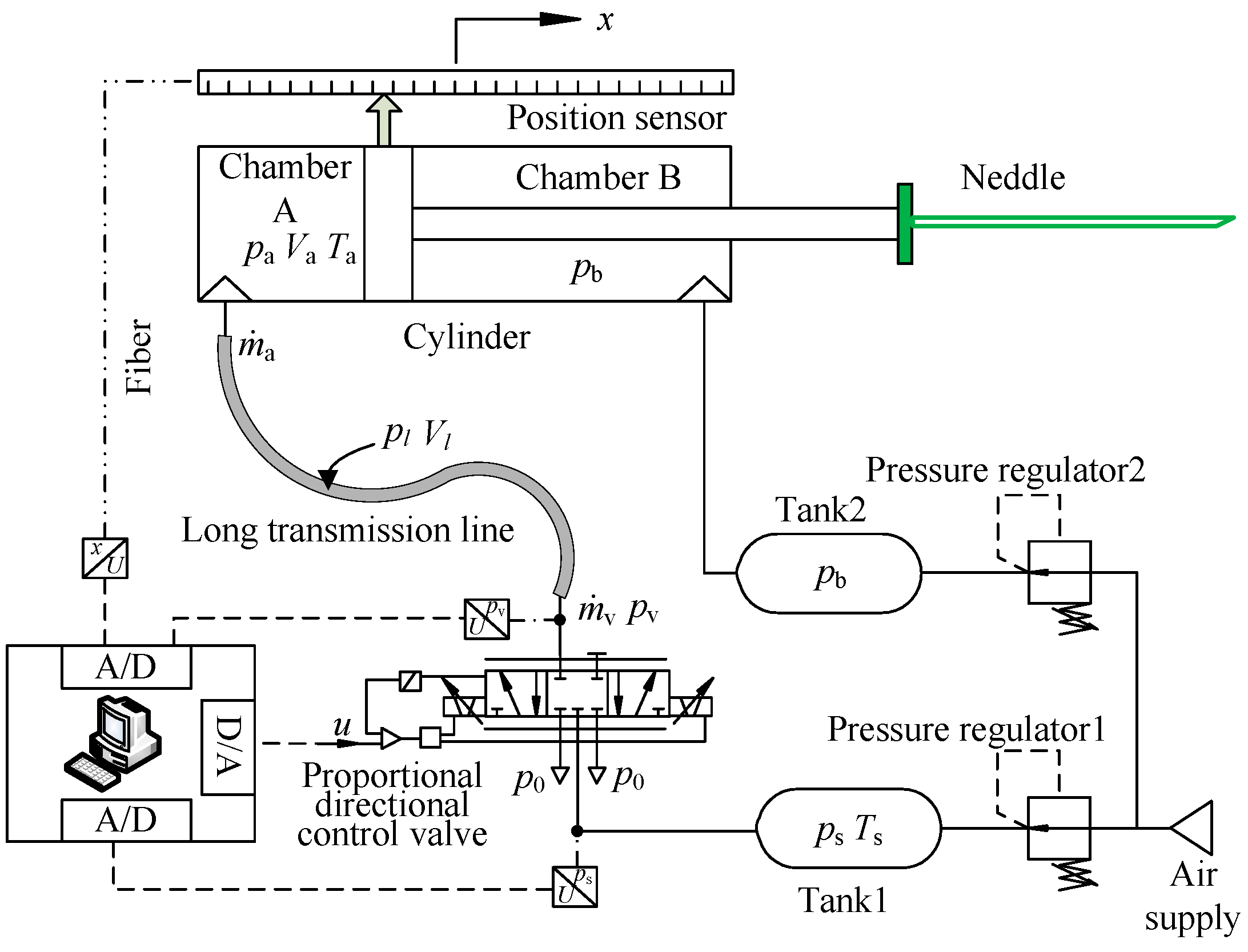
2. Dynamic Models and Problem Formulation

As shown in Figure 1, a 5-DOF (degree of freedom) MRI compatible robot for abdominal and thoracic punctures was built in our laboratory. The robot’s mechanism design was developed such that all motions were decoupled and actuated by pneumatic cylinders. With the help of the robot, the physician could manipulate the needle remotely without moving the patient out of the MRI scanners. A schematic of the pneumatic servo system driving the needle insertion motion is depicted in Figure 2. The pneumatic cylinder (customized product from XMC Corp., Ningbo, China), which had a 150 mm stroke and 10 mm diameter bore, was made of nonmagnetic material to ensure MRI compatibility. While Chamber A was controlled by a proportional directional control valve (FESTO MPYE-5-M5-010-B), a tank was used to maintain the pressure of Chamber B at a specified constant level for safety reasons. The control valve was connected to the cylinder via a 10 m transmission line since it had to be placed away from the MRI scanner. A pressure observer was needed to estimate the pressure of Chamber A, since direct measurement was expensive for the lack of MRI-compatible pressure sensors. The main purpose of this paper was to find a way to deal with the issue of the long transmission line and realize high accuracy control of a pneumatic cylinder with pressure observation. For the purpose of comparison, the pressures at the two ends of the long transmission line, as well as the supply pressure were measured by three pressure sensors (FESTO SDET-22T-D10-G14-I-M12). The piston position was obtained with an optical position sensor (Micronor MR328). The controller was programmed in Simulink on a dSPACE DS1103 control system with a 1 ms sampling period.
As shown in [34], the motion of the piston–rod–needle assembly can be expressed as:
m x ¨ = p a A a p b A b p 0 A r b x ˙ F f S f ( x ˙ ) d f ,
where x, x ˙ , and x ¨ are the piston position, velocity, and acceleration, respectively, m is the normal mass of the piston–rod–needle assembly, pa and pb denotes the absolute pressures of actuator chambers, p0 is the ambience pressure, Aa and Ab are the cross section areas of piston chambers, Ar is the cross section area of the rod, b is the total load and cylinder viscous friction coefficient, Ff is the unknown friction coefficient, Sf( x ˙ ) is a continuous function, which is always chosen as Sf( x ˙ ) = 2 π arctan ( 900 x ˙ ) , FfSf( x ˙ ) is utilized as the smooth approximation for the usual static discontinuous Coulomb friction force, and df represents the unmodeled dynamics and external disturbances.
With the assumption that the discharging and charging processes are both isothermal, the pressure dynamic in the actuator chamber can be modeled as [16,35]:
p ˙ a = R T s V a m ˙ a A a p a V a x ˙ , V a = V a 0 + A a ( L c 2 + x ) ,
where R is the gas constant, Ts is the ambient temperature, Va is the volume of the cylinder chamber A, m ˙ a is the mass flow entering or exiting the chamber A, Va0 is the dead volume of the cylinder chamber A, and Lc is stroke of the actuator. m ˙ a can be calculated by [16]:
m ˙ a = ( p l p a ) p v A l D l 32 R T s L l μ ,
where pl is the average air pressure in the transmission line, pv is the measured air pressure at the work port of the control valve, Ll, Al, and Dl denote the length, cross section area, and inner diameter of the transmission line, respectively, and μ is the dynamic viscosity of air.
As shown in Figure 2, the long transmission line is assumed to be an intermediate chamber connected between the control valve and the actuator in series, thus, the following equation is formulated to represent the pressure dynamic of the line [16,35]:
p ˙ l = R T s V l ( m ˙ v m ˙ a ) ,
where Vl is the volume of the transmission line, and m ˙ v is the mass flow rate through the valve, which can be calculated by [35]:
m ˙ v = A ( u ) K q ( p u , p d , T u ) = { A ( u ) C d C 1 p u T u , p d p u p r , A ( u ) C d C 1 p u T u 1 ( p d p u p r 1 p r ) 2 , p d p u > p r ,
where A(u) is the effective valve orifice area, u is the control valve’s control input, Cd is the discharge coefficient, C1 is a constant with a value of 0.0404, pu and pd are the upstream pressure and the downstream pressure, respectively, Tu is the upstream temperature of air, and pr is the critical pressure ratio. Therefore, m ˙ v = A ( u ) K q ( p s , p v , T s ) when the line is charging, and m ˙ v = A ( u ) K q ( p v , p 0 , T s ) when the line is discharging.
Choose the state vectors x = [x1, x2, x3, x4]T as x1 = x, x2 = x ˙ , x3 = pa and x4 = pl, thus the system dynamics can be expressed in a state-space form as:
{ x ˙ 1 = x 2 m x ˙ 2 = A a x 3 A b p b p 0 A r b x 2 A f S f ( x 2 ) d f x ˙ 3 = R T s V a m ˙ a A a x 2 V a x 3 x ˙ 4 = R T s V l ( m ˙ v m ˙ a ) .
The control objective is to synthesize a control input u for the system Equation (6) such that x tracks the desired trajectory xd with a guaranteed transient and final tracking accuracy. Instead of using the pressure sensor, a globally stable pressure observer is developed to estimate the pressure in chamber A. The parametric uncertainties due to unknown b and Af and unknown external disturbances will be explicitly considered in this paper.
Assumption 1:
The desired trajectory xd is at least second-order differentiable, and xd, x ˙ d , and x ¨ d are bounded. Then, there exists a compact set Ω 0 = { [ x d , x ˙ d , x ¨ d ] T : x d 2 + x ˙ d 2 + x ¨ d 2 B 0 } such that [ x d , x ˙ d , x ¨ d ] T Ω 0 , where B 0 is a positive constant.
Assumption 2:
The extent of parametric uncertainties and external disturbances can be predicted and given by b min b b max , F fmin F f F fmax ,and d min d f d max .

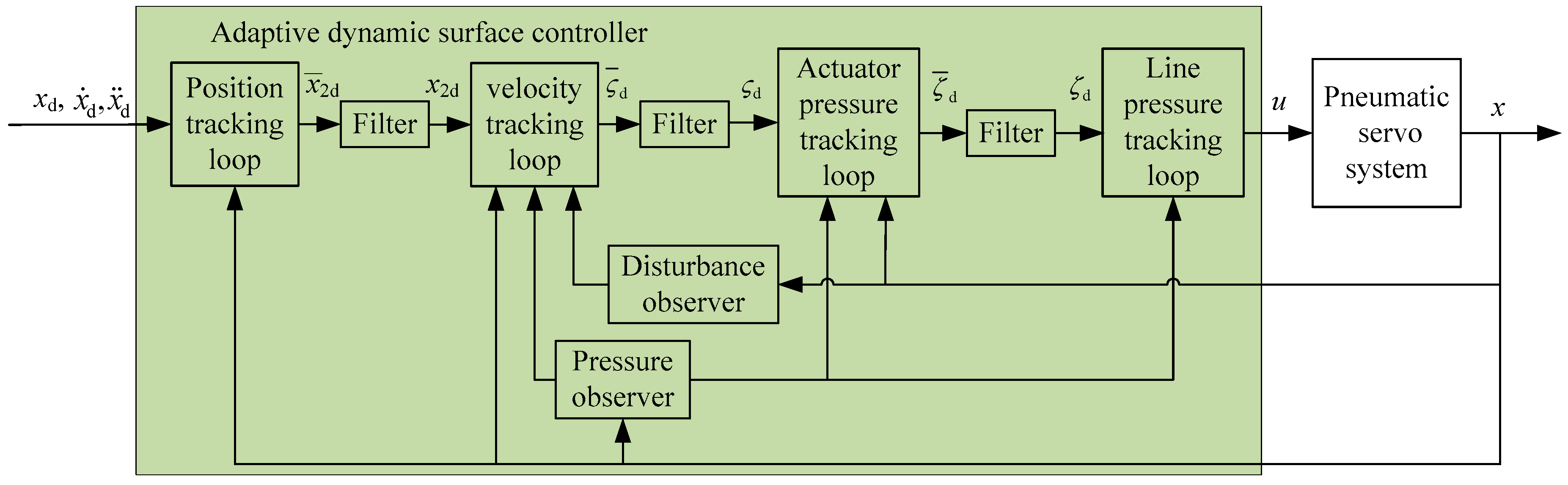
3. Controller Design

3.1. Pressure Observer

The following observer is proposed to estimate the pressure of the actuator chamber A and the average air pressure in the transmission line:
{ p ^ ˙ a = R T s V a m ˙ ^ a A a x ˙ V a p ^ a p ^ ˙ l = R T s V l ( m ˙ ^ v m ˙ ^ a ) ,
where p ^ a and p ^ l represent the estimates of p a and p l , m ˙ ^ a and m ˙ ^ v denote the estimated mass flow rates according to Equation (3) and Equation (5) based on p ^ a and p ^ l . It should be noted that the proposed observers are closed loop because of the relationship between the estimated mass flow rates and the estimated pressures. Proof of the convergence between the actual pressures and the estimated ones will be given later.
To verify the convergence between the actual pressures and the estimated pressures, the following Lyapunov function candidate was considered:
V o = V o 1 + V o 2 , V o 1 = 1 2 ( p ˜ a V a ) 2 , V o 2 = 1 2 ( p ˜ l V l ) 2 ,  
where p ˜ a = p a p ^ a , and p ˜ l = p l p ^ l .
The time derivative of V o 1 is:
V ˙ o 1 = ( p a V a p ^ a V a ) ( p ˙ a V a + p a V ˙ a p ^ ˙ a V a p ^ a V ˙ a ) = R T s V a ( p a p ^ a ) ( m ˙ a m ˙ ^ a )
According the Equation (3), one can obtain:
  • p a > p ^ a implies that m ˙ a < m ˙ ^ a , yielding ( p a p ^ a ) ( m ˙ a m ˙ ^ a ) < 0 .
  • p a < p ^ a implies that m ˙ a > m ˙ ^ a , yielding ( p a p ^ a ) ( m ˙ a m ˙ ^ a ) < 0 .
  • p a = p ^ a implies that m ˙ a < m ˙ ^ a , yielding ( p a p ^ a ) ( m ˙ a m ˙ ^ a ) = 0 .
Therefore, V ˙ o 1 is negative semi-definite.
The time derivative of V o 2 is:
V ˙ o 2 = ( p l V l p ^ l V l ) ( p ˙ l V l p ^ ˙ l V l ) = R T s V l ( p l p ^ l ) ( m ˙ v m ˙ ^ v ) R T s V l ( p l p ^ l ) ( m ˙ a m ˙ ^ a )
According the Equation (3), one can obtain:
  • p l > p ^ l implies that m ˙ a > m ˙ ^ a , yielding ( p l p ^ l ) ( m ˙ a m ˙ ^ a ) > 0 .
  • p l < p ^ l implies that m ˙ a < m ˙ ^ a , yielding ( p l p ^ l ) ( m ˙ a m ˙ ^ a ) > 0 .
  • p l = p ^ l implies that m ˙ a = m ˙ ^ a , yielding ( p l p ^ l ) ( m ˙ a m ˙ ^ a ) = 0 .
For the mass flow rate relationship given by Equation (5), it has proven in [25] that the term ( p l p ^ l ) ( m ˙ v m ˙ ^ v ) is always non-positive. Thus, V ˙ o 2 and V o are negative semi-definite, one can conclude that the proposed pressure observers are globally Lyapunov stable with regard to the errors in the estimated pressures.

3.2. Adaptive Dynamic Surface Controller

Step 1: Differentiate the trajectory tracking error e 1 = x 1 x d with respect to time leads to:
e ˙ 1 = x 2 x ˙ d .
Consider x2 as the first virtual control input, the virtual control law is designed as follows:
x ¯ 2 d = x ˙ d k 1 e 1 , k 1 > 0 ,
where k 1 is a positive control gain. Following the dynamic surface control theory [28], the signal x ¯ 2 d is fed to a low pass filter to obtain a new one x 2 d for the next design step:
τ 1 x ˙ 2 d + x 2 d = x ¯ 2 d , x 2 d ( 0 ) = x ¯ 2 d ( 0 ) , τ 1 > 0 ,
where τ 1 is the filter parameter.
Step 2: Define the first surface error as s 1 = x 2 x 2 d , its time derivative can be derived as:
s ˙ 1 = x ˙ 2 x ˙ 2 d = A ¯ a x 3 1 m [ p b A b + p 0 A r + b x 2 + F f S f ( x ˙ ) + d f ] 1 τ 1 ( x ¯ 2 d x 2 d ) ,
where A ¯ a = A a / m .
Define x ˜ 3 = x 3 x ^ 3 , and let ς = x ^ 3 be the second virtual control input, the virtual control law is designed as follows:
ς ¯ d = 1 A ¯ a { 1 m [ p b A b + p 0 A r + b ^ x 2 + F ^ f S f ( x ˙ ) + d ^ f ] + 1 τ 1 ( x ¯ 2 d x 2 d ) k 2 s 1 h 1 2 4 η 1 s 1 } ,
where k 2 > 0 is a positive control gain, η 1 > 0 is a controller parameter, and h1 is a known function that will be determined later, b ^ , F ^ f ,and d ^ f are the estimates of b, Ff, and df, respectively. b ^ , F ^ f , and d ^ f are updated by:
b ^ ˙ = Proj b ^ ( γ 1 m x 2 s 1 ) ,
F ^ ˙ f = Proj F ^ f ( γ 2 m S f ( x 2 ) s 1 ) ,
d ^ ˙ f = Proj d ^ f ( γ 3 m s 1 ) ,  
where γ 1 > 0 , γ 2 > 0 ,and γ 3 > 0 are the observer gains, and the projection mapping is defined as:
Proj ξ ^ ( ) = { 0 , if ξ ^ = ξ max and > 0 0 , if ξ ^ = ξ min and < 0 , otherwise ,
where ξ is a symbol that can be replaced by b, Ff, and df.
Similarly, the signal ς ¯ d is fed to a low pass filter to obtain a new one ς d for the next design step:
τ 2 ς ˙ d + ς d = ς ¯ d , ς d ( 0 ) = ς ¯ d ( 0 ) ,   τ 2 > 0 ,
where τ 2 is the filter parameter.
Step 3: Define the second surface error as s 2 = ς ς d , its time derivative can be derived as:
s ˙ 2 = ς ˙ ς ˙ d = x ^ ˙ 3 ς ˙ d = R T s V a m ˙ ^ a A a x 2 V a x ^ 3 1 τ 2 ( ς ¯ d ς d ) = R T s a V a x ^ 4 + ( R T s a V a A a x 2 V a ) x ^ 3 1 τ 2 ( ς ¯ d ς d )
where a = p v A l D l 32 R T s L l μ .
Let ζ = x ^ 4 be the third virtual control input, the virtual control law is designed as follows:
ζ ¯ d = V a R T s a [ ( A a x 2 V a R T s a V a ) x ^ 3 + 1 τ 2 ( ς ¯ d ς d ) k 3 s 2 ] ,
where k 3 > 0 is a positive control gain. Similarly, the signal ζ ¯ d is fed to a low pass filter to obtain a new one ζ d for the next design step:
τ 3 ζ ˙ d + ζ d = ζ ¯ d , ζ d ( 0 ) = ζ ¯ d ( 0 ) ,   τ 3 > 0 ,
where τ 3 is the filter parameter.
Step 4: Define the second surface error as s 3 = ζ ζ d , its time derivative can be derived as:
s ˙ 3 = ζ ˙ ζ ˙ d = x ^ ˙ 4 ζ ˙ d = R T s V l ( m ˙ ^ v m ˙ ^ a ) 1 τ 3 ( ζ ¯ d ζ d ) .
Similarly, the following control law qd for m ˙ ^ v is proposed:
q d = m ˙ ^ a R T s V l [ 1 τ 3 ( ζ ¯ d ζ d ) k 4 s 3 ] ,  
where k 4 > 0 is a positive control gain.
Once the qd is calculated, the desired effective valve orifice area A(u) can be calculated by:
A ( u ) = { q d K q ( p s , p v , T s ) q d > 0 q d K q ( p v , p 0 , T s ) q d 0 .
Thus, the input signal u for the proportional-directional control valve could be obtained according to the relation between the input signal and effective valve orifice area.
The proposed pressure observer based adaptive dynamic surface control is illustrated in Figure 3.

3.3. Proof of Stability

Theorem 1.
Consider the closed loop pneumatic servo system consisting of the plant Equation (6), the nonlinear control law Equation (25), the pressure observers Equation (7), and the parameter and disturbance estimation algorithm Equations (16)–(18) under the Assumption 1–2. If there exists a set of the feedback gains and the filter constants satisfying γ = min { k 1 1 , k 2 1 2 A ¯ a , k 3 A ¯ a 2 , 1 τ 1 1 , 1 τ 2 1 2 A ¯ a 2 } > 0 , then the closed loop system is uniformly and ultimately bounded.
Proof. 
Consider the following Lyapunov function candidate:
V c = V cs + V cz + V θ , V cs = 1 2 e 1 2 + 1 2 s 1 2 + 1 2 s 2 2 + 1 2 s 3 2 , V cz = 1 2 z 1 2 + 1 2 z 2 2 + 1 2 z 3 2 , V θ = 1 2 γ 1 1 b ˜ 2 + 1 2 γ 2 1 F ˜ f 2 + 1 2 γ 3 1 d ˜ f 2
where z 1 = x 2 d x ¯ 2 d , z 2 = ς d ς ¯ d , z 3 = ζ d ζ ¯ d . Substituting Equation (12) into Equation (11) gives:
e ˙ 1 = s 1 + z 1 k 1 e 1 .
Substituting Equation (15) into Equation (14) and noting x ^ 3 = s 2 + ς d = s 2 + z 2 + ς ¯ d yields:
s ˙ 1 = A ¯ a ( s 2 + z 2 ) 1 m [ b ˜ x 2 + F ˜ f S f ( x ˙ ) + d ˜ f ] + A ¯ a x ˜ 3 k 2 s 1 h 1 2 4 η 1 s 1 ,
where b ˜ = b b ^ , F ˜ f = F f F ^ f , d ˜ f = d f d ^ f .
Substituting Equation (22) into Equation (21) and noting x ^ 4 = s 3 + ζ d = s 3 + z 3 + ζ ¯ d yields:
s ˙ 2 = R T s a V a ( s 3 + z 3 ) k 3 s 2 .
Substituting Equation (25) into Equation (24) gives:
s ˙ 3 = k 4 s 3 .
Therefore, the time derivative of V 1 = V cs + V θ is:
V ˙ 1 = k 1 e 1 2 k 2 s 1 2 k 3 s 2 2 k 4 s 3 2 + e 1 s 1 + e 1 z 1 + A ¯ a ( s 1 s 2 + s 1 z 2 ) + R T s a V a ( s 3 + z 3 ) + γ 1 1 b ˜ [ b ^ ˙ ( γ 1 m x 2 s 1 ) ] + γ 2 1 F ˜ f [ F ^ ˙ f ( γ 2 m S f ( x 2 ) s 1 ) ] + γ 3 1 d ˜ f [ d ^ ˙ f ( γ 3 m s 1 ) ] + s 1 { h 1 2 4 η 1 s 1 1 m [ b ˜ x 2 + F ˜ f S f ( x ˙ ) + d ˜ f ] + A ¯ a x ˜ 3 }
It has been proved in [36] that with the projection mapping, the following properties hold:
b ˜ [ Proj b ^ ( γ 1 m x 2 s 1 ) ( γ 1 m x 2 s 1 ) ] 0 .
F ˜ f [ Proj F ^ f ( γ 2 m S f ( x 2 ) s 1 ) ( γ 2 m S f ( x 2 ) s 1 ) ] 0 .
d ˜ f [ Proj d ^ f ( γ 3 m s 1 ) ( γ 3 m s 1 ) ] 0 .
According to Assumption 1–2, there exists a known function h1 satisfies:
h 1 ( t ) 1 m [ | b max b min | | x 2 | + | F fmax F fmin | | S f ( x 2 ) | + | d max d min | ] + A ¯ a | ρ 1 | ,  
where ρ 1 is the bound of x ˜ 3 as proven in the above step. From the smoothed sliding mode control theory, the following inequality holds.
s 1 { h 1 2 4 η 1 s 1 1 m [ b ˜ x 2 + F ˜ f S f ( x ˙ ) + d ˜ f ] + A ¯ a x ˜ 3 } η 1 .
Substituting Equation (34) into Equation (32) yields
V ˙ 1 k 1 e 1 2 k 2 s 1 2 k 3 s 2 2 k 4 s 3 2 + e 1 s 1 + e 1 z 1 + A ¯ a ( s 1 s 2 + s 1 z 2 ) + R T s a V a ( s 3 + z 3 ) + η 1 .
The following inequalities can be obtained by using Young’s inequality.
e 1 s 1 e 1 2 2 + s 1 2 2 , e 1 z 1 e 1 2 2 + z 1 2 2 , s 1 s 2 s 1 2 2 + s 2 2 2 s 1 z 2 s 1 2 2 + z 2 2 2 , s 2 s 3 s 2 2 2 + s 3 2 2 , s 2 z 3 s 2 2 2 + z 3 2 2
Substituting Equation (37) into Equation (36) gives:
V ˙ 1 ( k 1 1 ) e 1 2 ( k 2 1 2 A ¯ a ) s 1 2 ( k 3 A ¯ a 2 R T s a V a ) s 2 2 ( k 4 R T s a 2 V a ) s 3 2 + 1 2 z 1 2 + A ¯ a 2 z 2 2 + R T s a 2 V a z 3 2 + η 1
Following the similar analysis as done in [28], the following inequalities hold.
z ˙ 1 + z 1 τ 1 | z ˙ 1 + z 1 τ 1 | ξ 1 , z ˙ 2 + z 2 τ 2 | z ˙ 2 + z 2 τ 2 | ξ 2 , z ˙ 3 + z 3 τ 3 | z ˙ 3 + z 3 τ 3 | ξ 3 ,
where ξ 1 ( e 1 , s 1 , z 1 , x d , x ˙ d , x ¨ d ) , ξ 2 ( e 1 , s 1 , s 2 , z 1 , z 2 , x d , x ˙ d , x ¨ d ) , and ξ 2 ( e 1 , s 1 , s 2 , s 3 , z 1 , z 2 , z 3 , x d , x ˙ d , x ¨ d ) are three continuous functions. Due to the fact that the set Ω 0 is compact in R 3 and the set Ω 1 = { [ e 1 , s 1 , s 2 , s 3 , z 1 , z 2 , z 3 ] T : e 1 2 + s 1 2 + s 2 2 + s 3 2 + z 1 2 + z 2 2 + z 3 2 2 B 1 } (where B 1 > 0) is compact in R 7 , Ω 0 × Ω 1 is thus compact in R 10 . Therefore, ξ 1 , ξ 2 , and ξ 3 have maximums on Ω 0 × Ω 1 . Let M1, M2, and M3 be the maximums of ξ 1 , ξ 2 , and ξ 3 on Ω 0 × Ω 1 , respectively, one can obtain that:
z 1 z ˙ 1 + z 1 2 τ 1 M 1 | z 1 | , z 2 z ˙ 2 + z 2 2 τ 2 M 2 | z 2 | , z 3 z ˙ 3 + z 3 2 τ 3 M 3 | z 3 | .
With the use of Young’s inequality, one can obtain that:
z 1 z ˙ 1 z 1 2 τ 1 + z 1 2 2 + M 1 2 2 , z 2 z ˙ 2 z 2 2 τ 2 + z 2 2 2 + M 2 2 2 , z 3 z ˙ 3 z 3 2 τ 3 + z 3 2 2 + M 3 2 2 .
Thus, the following inequalities can be obtained.
V ˙ cz 1 τ 1 z 1 2 1 τ 2 z 2 2 1 τ 3 z 3 2 + 1 2 z 1 2 + 1 2 M 1 2 + 1 2 z 2 2 + 1 2 M 2 2 + 1 2 z 3 2 + 1 2 M 3 2 .
Thus, the following inequalities can be obtained.
V ˙ 1 ( k 1 1 ) e 1 2 ( k 2 1 2 A ¯ a ) s 1 2 ( k 3 A ¯ a 2 R T s a V a ) s 2 2 ( k 4 R T s a 2 V a ) s 3 2 ( 1 τ 1 1 ) z 1 2 ( 1 τ 2 1 2 A ¯ a 2 ) z 2 2 ( 1 τ 3 1 2 R T s a 2 V a ) z 3 2 + 1 2 M 1 2 + 1 2 M 2 2 + 1 2 M 3 2 + η 1
By choosing k 1 > 1 , k 2 > 1 2 + A ¯ a , k 3 > A ¯ a 2 + R T s a V a , k 4 > R T s a 2 V a , τ 1 < 1 , τ 2 < 2 A ¯ a + 1 , and τ 3 < 2 V a R T s a + V a , one has:
γ = min { k 1 1 , k 2 1 2 A ¯ a , k 3 A ¯ a 2 R T s a V a , k 4 R T s a 2 V a , 1 τ 1 1 , 1 τ 2 1 2 A ¯ a 2 , 1 τ 3 1 2 R T s a 2 V a } > 0
Then, it can be readily obtained that the following inequality holds.
V ˙ 2 γ V + η ,
where η = 1 2 M 1 2 + 1 2 M 2 2 + 1 2 M 3 2 + η 1 . □
Clearly, if γ > η / 2 B 1 , then V ˙ 0 on set Ω 1 , thus V will remain V ( t ) B 1 for all t, provided that the initial conditions satisfy V ( 0 ) B 1 . Therefore, the errors e 1 , s 1 , s 2 , s 3 , z 1 , z 2 , z 3 are bounded. Hence, one can conclude that the closed loop system is uniformly and ultimately bounded.

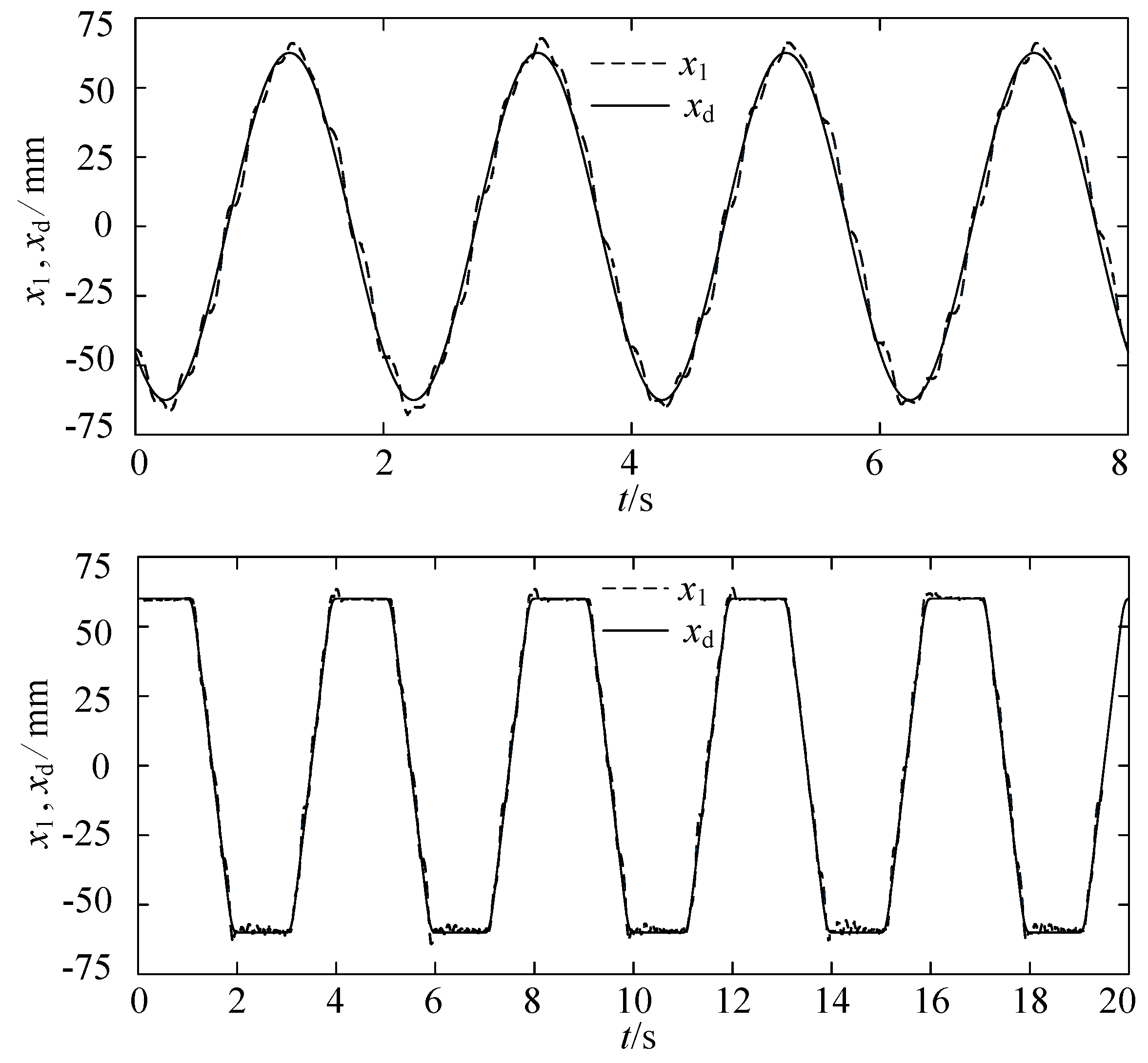
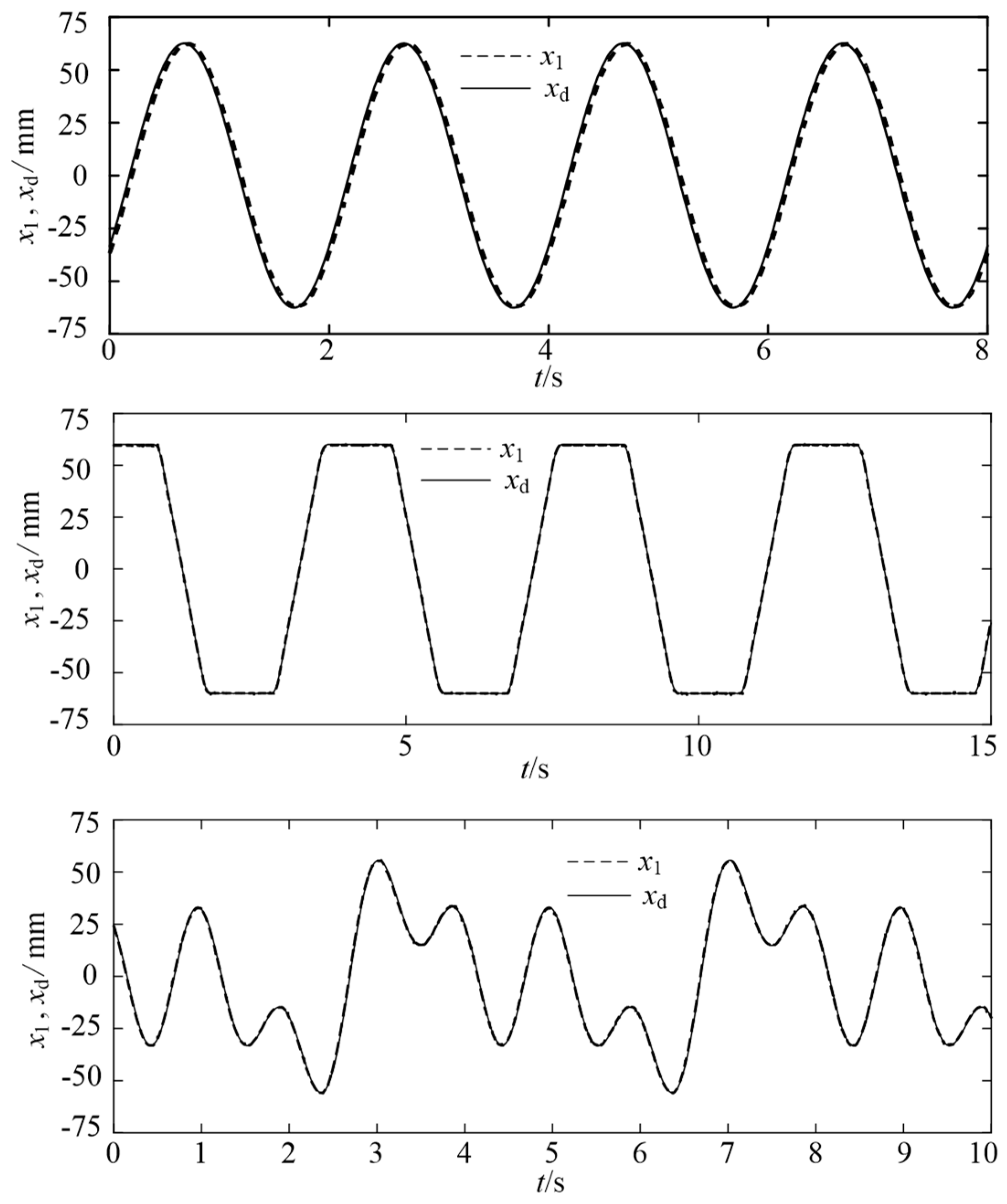
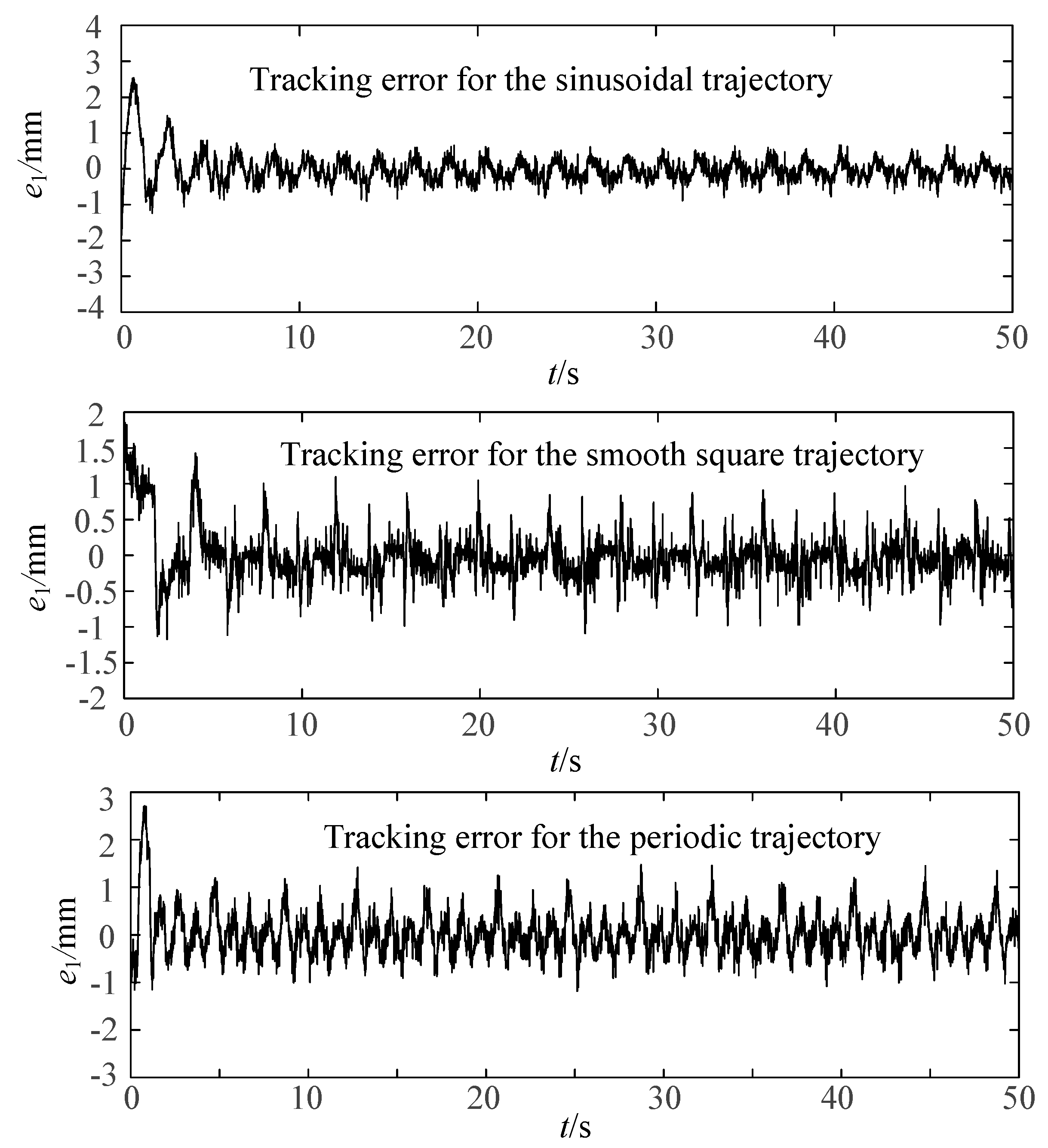
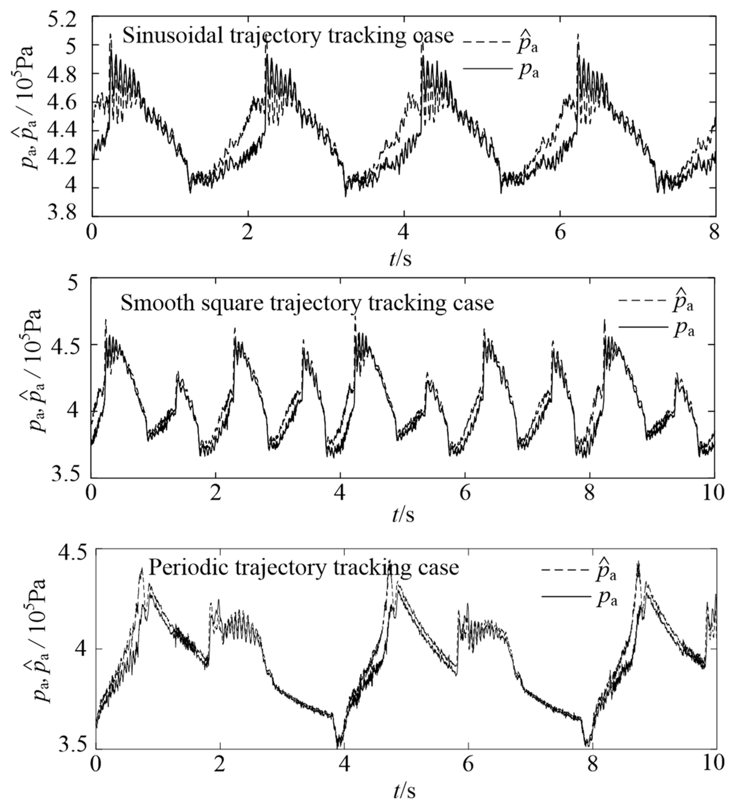
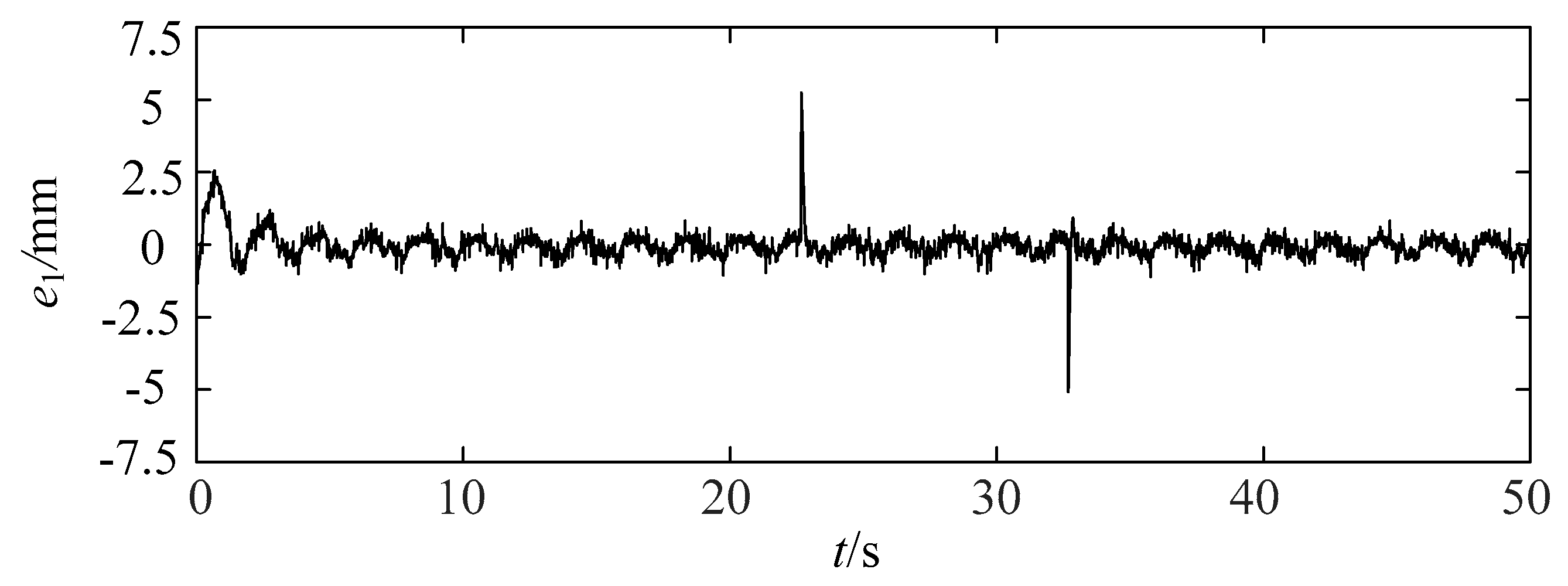
4. Experimental Results

In this section, the proposed controller was implemented for the servo control of the pneumatic servo system as shown in Figure 2. The cylinder forward chamber was controlled by the valve through a 10 m long transmission line with 4 mm inside diameter, while the pressure in the return chamber was maintained at about 3 bar by utilizing a tank. A gel phantom was used to perform the following needle insertion experiments. The system physical parameters and the parameters of the controller are given in Table 1.
The same control algorithm as the proposed controller, but in which the long transmission line was characterized as a part of the cylinder’s dead volume and the chamber pressure was directly measured, was first tested for tracking a sinusoidal trajectory and a smooth square trajectory. As shown in Figure 4, the performance was poor for practical application, which indicates the need for an advanced method to address the issue of long transmission line. The performance of the proposed controller was tested on three types of reference trajectories: A 0.5 Hz sinusoidal signal, a smooth square signal, and a 4 s periodic signal. Figure 5 shows the response of the system, and the tracking errors are presented in Figure 6. The maximum absolute tracking errors ( max t { | e 1 | } ) were about 2.51 mm, 2.68 mm, and 1.81 mm, while the final steady-state tracking errors ( max t 5 { | e 1 | } ) were about 0.96 mm, 1.05 mm, and 1.39 mm. As seen, the proposed controller could significantly improve the system performance, which indicates the effectiveness of the proposed long transmission line compensation method. However, it should be noted that these needle insertion experiments were performed in a gel phantom, whose resisting force behavior was simpler than real soft tissue. The interaction between needle and soft tissue is very complex and may decrease the needle insertion precision in practical. Since the current research focused on addressing the issue of long transmission line and realizing high accuracy control of a pneumatic actuator with a pressure observer, modeling of needle-tissue interaction and further improving needle insertion precision would be the subject of the next phase of this research.
The process of parameter and disturbance estimations is shown in Figure 7. It can be seen that the estimates converged quickly, and the tracking error improvement could be achieved within several seconds. Comparisons between the observed chamber pressure and the measured one are shown in Figure 8. As can be seen, the estimated chamber pressure was close to its actual value, which indicates the effectiveness of the proposed pressure observer. However, the estimation error during the charging process was slightly bigger than the one during the discharging process. This might be due to the fact that charging process was close to adiabatic and the discharging process was close to isothermal.
Experiments were also conducted to verify the performance robustness of the proposed controller. To simulate a sudden disturbance acting on the system, a big step signal was added to the output of the position sensor at t = 22 s, and removed 10 s later. Figure 9 shows the control accuracy of the proposed controller in this scenario for tracking a sinusoidal trajectory with a frequency of 0.5 Hz and amplitude of 62.5 mm. It can be seen that the system performance did not deteriorate except the transient spikes when the sudden disturbance was added or removed.

5. Conclusions

In this paper, the precise motion control of a MRI compatible 1-DOF pneumatic servo system was considered. The long transmission line was characterized as an intermediate chamber connected between the valve and the cylinder in series, and a nonlinear first order system was used to approximate its dynamics. Simultaneously, a globally stable pressure observer was developed to estimate the chamber pressure. Based on the model of the long transmission line and the pressure observer, a pressure observer based adaptive dynamic surface controller was developed and the stability of the closed-loop system was proved via the Lyapunov method. In contrast to most of the existing nonlinear controllers synthesized with the backstepping method, by employing the dynamic surface control technique, the proposed controller could cope with the problem of “explosion of complexity”, since the repeated differentiation of virtual controls was no longer required. The experimental results confirmed that the proposed controller was effective and had good performance robustness to sudden disturbances, thus enabling future application in pneumatically actuated MRI-compatible robots. However, precise motion control of pneumatic actuator did not necessarily lead to precise position control needle tip. Modeling of the interaction between needle and soft tissue, and incorporating a more accurate needle insertion force model in the controller design is an essential requirement for practical robot-assisted needle insertion. Thus, these issues will be explored further in the next phase of this research.

Author Contributions

D.M. and B.L. proposed the pressure observe based dynamic surface controller for precise position tracking control of the MRI-compatible pneumatic servo system. A.L. designed the experiments. J.Y. and Q.L. performed the experiments and analyzed the data. D.M. and A.L. wrote the paper.

Funding

This research was funded by [the Fundamental Research Funds for the Central Universities] grant number [2015XKMS020], [the National Natural Science Foundation of China] grant number [51505474], [the China Postdoctoral Science Foundation ] grant number [2016T90520], and [a Project Funded by the Priority Academic Program Development of Jiangsu Higher Education Institutions]. And the APC was funded by the Fundamental Research Funds for the Central Universities.

Acknowledgments

This work was supported by the National Natural Science Foundation of China (Grant No. 51505474), the Fundamental Research Funds for the Central Universities (Grant No. 2015XKMS020), the China Postdoctoral Science Foundation (Grant No. 2016T90520), and a Project Funded by the Priority Academic Program Development of Jiangsu Higher Education Institutions.

Conflicts of Interest

The authors declare no conflict of interest.

References

  1. Fischer, G.; Iordachita, I.; Csoma, C.; Tokuda, J.; DiMaio, S.; Tempany, C.; Hata, N.; Fichtinger, G. MRI-compatible pneumatic robot for transperineal prostate needle placement. IEEE/ASME Trans. Mechatron. 2008, 13, 295–305. [Google Scholar] [CrossRef] [PubMed]
  2. Stoianovici, D.; Jun, C.; Lim, S.; Li, P.; Petrisor, D.; Fricke, S.; Sharma, K.; Cleary, K. Multi-image compatible, MR safe, remote center of motion needle-guide robot. IEEE Trans. Biomed. Eng. 2018, 65, 165–177. [Google Scholar] [CrossRef] [PubMed]
  3. Stoianovici, D.; Kim, C.; Srimathveeravalli, G.; Sebrecht, P.; Petrisor, D.; Coleman, J.; Solomon, S.; Hricak, H. MRI-Safe Robot for Endorectal Prostate Biopsy. Trans. Mechatron. 2014, 19, 1289–1299. [Google Scholar] [CrossRef]
  4. Stoianovici, D.; Patriciu, A.; Petrisor, D.; Mazilu, D.; Kavoussi, L. A new type of motor: Pneumatic step motor. IEEE/ASME Trans. Mechatron. 2007, 12, 98–106. [Google Scholar] [CrossRef] [PubMed]
  5. Zemiti, N.; Bricault, I.; Fouard, C.; Sanchez, B.; Cinquin, P. LPR: A CT and MR-compatible puncture robot to enhance accuracy and safety of image-guided interventions. IEEE/ASME Trans. Mechatron. 2008, 13, 306–315. [Google Scholar] [CrossRef]
  6. Schouten, M.; Bomers, J.; Yakar, D.; Huisman, H.; Rothgang, E.; Bosboom, D.; Scheenen, T.; Misra, S.; Futterer, J. Evaluation of a robotic technique for transrectal MRI-guided prostate biopsies. Eur. Radiol. 2012, 22, 476–483. [Google Scholar] [CrossRef] [PubMed]
  7. Franco, E.; Brujic, D.; Rea, M.; Gedroyc, W.; Ristic, M. Needle-guiding robot for laser ablation of liver tumors under MRI guidance. IEEE/ASME Trans. Mechatron. 2016, 21, 931–944. [Google Scholar] [CrossRef]
  8. Yang, B.; Tan, U.; McMillan, A.; Gullapalli, R.; Desai, J. Design and control of a 1-DOF MRI-compatible pneumatically actuated robot with long transmission lines. IEEE/ASME Trans. Mechatron. 2011, 16, 1040–1048. [Google Scholar] [CrossRef] [PubMed]
  9. Yang, B.; Roys, S.; Tan, U.; Philip, M.; Richard, H.; Gullapalli, R.; Desai, J. Design, development, and evaluation of a master–slave surgical system for breast biopsy under continuous MRI. Int. J. Robot. Res. 2014, 33, 616–630. [Google Scholar] [CrossRef]
  10. Van den Bosch, M.; Moman, M.; van Vulpen, M.; Battermann, J.; Duiveman, E.; van Schelven, L.; de Leeuw, H.; Lagendijk, J.; Moerland, M. MRI-guided robotic system for transperineal prostate interventions: Proof of principle. Phys. Med. Biol. 2010, 55, 133–140. [Google Scholar] [CrossRef]
  11. Chen, Y.; Squires, A.; Seifabadi, R.; Xu, S.; Agarwal, H.; Bernardo, M.; Pinto, P.; Choyke, P.; Wood, B.; Tse, Z. Robotic system for MRI-guided focal laser ablation in the prostate. IEEE/ASME Trans. Mechatron. 2017, 22, 107–114. [Google Scholar] [CrossRef] [PubMed]
  12. Chen, Y.; Xu, S.; Squires, A.; Seifabadi, R.; Turkbey, I.; Pinto, P.; Choyke, P.; Wood, B.; Tse, Z. MRI-guided robotically assisted focal laser ablation of the prostate using canine cadavers. IEEE/ASME Trans. Mechatron. 2018, 65, 1434–1442. [Google Scholar] [CrossRef] [PubMed]
  13. Melzer, A.; Gutmann, B.; Remmele, T.; Wolf, R.; Lukoscheck, A.; Bock, M.; Bardenheuer, H.; Fischer, H. INNOMOTION for percutaneous image-guided interventions. IEEE Eng. Med. Biol. Mag. 2008, 27, 66–73. [Google Scholar] [CrossRef] [PubMed]
  14. Jiang, S.; Feng, W.; Lou, J.; Yang, Z.; Liu, J.; Yang, J. Modeling and control of a five-degrees-of-freedom pneumatically actuated magnetic resonance-compatible robot. Int. J. Med. Robot. Comput. Assist. Surg. 2014, 10, 170–179. [Google Scholar] [CrossRef] [PubMed]
  15. Comber, D.; Barth, E.; Webster, R. Design and control of a magnetic resonance compatible precision pneumatic active cannula robot. J. Med. Dev. 2014, 8, 1011003-1–1011003-7. [Google Scholar] [CrossRef]
  16. Richer, E.; Hurmuzlu, Y. A high performance pneumatic force actuator system: Part 1—nonlinear mathematical model. J. Dyn. Syst. Meas. Control 2000, 122, 416–425. [Google Scholar] [CrossRef]
  17. Richer, E.; Hurmuzlu, Y. A high performance pneumatic force actuator system: Part II—nonlinear controller design. J. Dyn. Syst. Meas. Control 2000, 122, 426–434. [Google Scholar] [CrossRef]
  18. Turkseven, M.; Ueda, J. An asymptotically stable pressure observer based on load and displacement sensing for pneumatic actuators with long transmission lines. IEEE/ASME Trans. Mechatron. 2017, 22, 681–692. [Google Scholar] [CrossRef]
  19. Li, J.; Kawashima, K.; Fujita, T.; Kagawa, T. Control design of a pneumatic cylinder with distributed model of pipelines. Precis. Eng. 2013, 37, 880–887. [Google Scholar] [CrossRef]
  20. Krichel, S.; Sawodny, O. Non-linear friction modeling and simulation of long pneumatic transmission lines. Math. Comput. Model. Dyn. Syst. 2014, 20, 23–44. [Google Scholar] [CrossRef]
  21. Turkseven, M.; Ueda, J. Model-based force control of pneumatic actuators with long transmission lines. IEEE/ASME Trans. Mechatron. 2018, 23, 1292–1302. [Google Scholar] [CrossRef]
  22. Pandian, S.; Takemura, F.; Hayakawa, Y.; Kawamura, S. Pressure observer-controller design for pneumatic cylinder actuators. IEEE/ASME Trans. Mechatron. 2002, 7, 490–499. [Google Scholar] [CrossRef]
  23. Wu, J.; Goldfarb, M.; Barth, E. On the observability of pressure in a pneumatic servo actuator. J. Dyn. Syst. Meas. Control 2004, 126, 921–924. [Google Scholar] [CrossRef]
  24. Bigras, P. Sliding-mode observer as a time-variant estimator for control of pneumatic systems. J. Dyn. Syst. Meas. Control 2005, 127, 499–502. [Google Scholar] [CrossRef]
  25. Gulati, N.; Barth, E. A globally stable, load-independent pressure observer for the servo control of pneumatic actuators. IEEE/ASME Trans. Mechatron. 2009, 14, 295–306. [Google Scholar] [CrossRef]
  26. Langjord, H.; Kassa, G.; Johansen, T. Adaptive nonlinear observer for electropneumatic clutch actuator with position sensor. IEEE Trans. Control Syst. Technol. 2012, 20, 1033–1039. [Google Scholar] [CrossRef]
  27. Driver, T.; Shen, X. Pressure estimation-based robust force control of pneumatic actuators. Int. J. Fluid Power 2013, 14, 37–45. [Google Scholar] [CrossRef]
  28. Swaroop, D.; Hedrick, J.K.; Yip, P.P.; Gerdes, J.C. Dynamic surface control for a class of nonlinear systems. IEEE Trans. Autom. Control 2000, 45, 1893–1899. [Google Scholar] [CrossRef] [Green Version]
  29. Kheowree, T.; Kuntanapreeda, S. Adaptive dynamic surface control of an electrohydraulic actuator with friction compensation. Asian J. Control 2015, 17, 855–867. [Google Scholar] [CrossRef]
  30. Peng, Z.; Wang, D.; Chen, Z.; Hu, X.; Lan, W. Adaptive dynamic surface control for formations of autonomous surface vehicles with uncertain dynamics. IEEE Trans. Control Syst. Technol. 2013, 21, 513–520. [Google Scholar] [CrossRef]
  31. Huang, J.; Ri, S.; Liu, L.; Wang, Y.; Kim, Y.; Pak, G. Nonlinear disturbance observer-based dynamic surface control of mobile wheeled inverted pendulum. IEEE Trans. Control Syst. Technol. 2015, 23, 2400–2407. [Google Scholar] [CrossRef]
  32. Wu, J.; Huang, J.; Wang, Y.; Xing, K. Nonlinear disturbance observer-based dynamic surface control for trajectory tracking of pneumatic muscle system. IEEE Trans. Control Syst. Technol. 2014, 22, 440–455. [Google Scholar] [CrossRef]
  33. Wang, M.; Ren, X.; Chen, Q.; Wang, S.; Gao, X. Modified dynamic surface approach with bias torque for multi-motor servomechanism. Control Eng. Pract. 2016, 50, 57–68. [Google Scholar] [CrossRef]
  34. Li, A.; Meng, D.; Lu, B.; Li, Q. Nonlinear cascade control of single-rod pneumatic actuator based on an extended disturbance observer. J. Cent. South Univ. 2019, 26, 1637–1648. [Google Scholar] [CrossRef]
  35. Meng, D.; Tao, G.; Chen, J.; Ban, W. Modeling of a pneumatic system for high-accuracy position control. In Proceedings of the International Conference on Fluid Power and Mechatronics, Beijing, China, 17–20 August 2011; pp. 505–510. [Google Scholar]
  36. Goodwin, G.; Mayne, D. A parameter estimation perspective of continuous time model reference adaptive control. Automatica 1989, 23, 57–70. [Google Scholar] [CrossRef]
Figure 1. Virtual prototype of a 5-DOF (degree of freedom) magnetic resonance imaging (MRI) compatible robot for abdominal and thoracic punctures.
Applsci 09 03621 g001
Figure 2. Schematic of the pneumatic servo system used to drive the needle insertion motion.
Applsci 09 03621 g002
Figure 3. Block diagram of the control system.
Applsci 09 03621 g003
Figure 4. Tracking response of the same control algorithm as the proposed controller but without using long transmission line compensation.
Applsci 09 03621 g004
Figure 5. Tracking response of the proposed controller for three different types of trajectories.
Applsci 09 03621 g005
Figure 6. Tracking errors of the proposed controller for three different types of trajectories.
Applsci 09 03621 g006
Figure 7. Parameter and disturbance estimations of the proposed controller when the reference is a 0.5 Hz sinusoidal trajectory.
Applsci 09 03621 g007
Figure 8. Actual and observed chamber pressure for the system tracking three different types of references.
Applsci 09 03621 g008
Figure 9. Tracking error of the proposed controller for 0.5 Hz sinusoidal trajectory with disturbance.
Applsci 09 03621 g009
Table 1. Parameters of the system and the proposed controller.
SymbolValueUnit
m0.32kg
Aa7.854 × 10−5m2
Ab6.597 × 10−4m2
Ar1.257 × 10−5m2
R287N m/(kg K)
Ts300K
ps6 × 105Pa
Va06 × 10−7m3
Lc0.125m
Vl1.257 × 10−4m3
Cd1.099 − 0.1075 × p u p d
pr0.29
Al1.257 × 10−5m2
Dl0.004m
Ll10m
μ 1.79 × 10⁻⁵N s/m2
p01 × 105Pa
b ^ ( 0 ) , b min , b max 9, 0, 15N s/m
F ^ f ( 0 ) , F ^ f min , F ^ f max 6, 0, 20N
d ^ f ( 0 ) , d min , d max 0, −10, 10N
k1, τ 1 40, 0.5
k2, h1, η 1 , τ 2 50, 40, 0.4, 0.75
k3, τ 3 50, 1.2
k490
γ 1 , γ 2 , γ 3 100, 10, 10

