Article

Semi-Supervised Convolutional Neural Network for Law Advice Online

1
The School of Computer Science and Technology, Chongqing University of Posts and Telecommunications, Chongqing 400065, China
2
The College of Automation, Chongqing University of Posts and Telecommunications, Chongqing 400065, China
*
Author to whom correspondence should be addressed.
These authors contributed equally to this work.
Appl. Sci. 2019, 9(17), 3617; https://doi.org/10.3390/app9173617
Submission received: 31 July 2019 / Revised: 26 August 2019 / Accepted: 28 August 2019 / Published: 3 September 2019

Abstract

:
With the rapid developments of Internet technology, a mass of law cases is constantly occurring and needs to be dealt with in time. Automatic classification of law text is the most basic and critical process in the online law advice platform. Deep neural network-based natural language processing (DNN-NLP) is one of the most promising approaches to implement text classification. Meanwhile, as the convolutional neural network-based (CNN-based) methods developed, CNN-based text classification has already achieved impressive results. However, previous work applied amounts of manually-annotated data, which increased the labor cost and reduced the adaptability of the approach. Hence, we present a new semi-supervised model to solve the problem of data annotation. Our method learns the embedding of small text regions from unlabeled data and then integrates the learned embedding into the supervised training. More specifically, the learned embedding regions with the two-view-embedding model are used as an additional input to the CNN’s convolution layer. In addition, to implement the multi-task learning task, we propose the multi-label classification algorithm to assign multiple labels to an instance. The proposed method is evaluated experimentally subject to a law case description dataset and English standard dataset RCV1 . On Chinese data, the simulation results demonstrate that, compared with the existing methods such as linear SVM, our scheme respectively improves by 7.76%, 7.86%, 9.19%, and 2.96% the precision, recall, F-1, and Hamming loss. Analogously, the results suggest that compared to CNN, our scheme respectively improves by 4.46%, 5.76%, 5.14% and 0.87% in terms of precision, recall, F-1, and Hamming loss. It is worth mentioning that the robustness of this method makes it suitable and effective for automatic classification of law text. Furthermore, the design concept proposed is promising, which can be utilized in other real-world applications such as news classification and public opinion monitoring.

1. Introduction

With the progress of information technology and the rapid development of Web2.0 network technology, the incredible development of the Internet has changed people’s lives, entertainment, and consumption pattern greatly. At present, as more and more users are willing to carry out online law advice, law case handling, and other services, several kinds of law service patterns were shown in [1,2]. How to find useful information quickly and accurately from law case description becomes very important for law text classification [3,4]. An decision support online law consulting platform is necessary to automatically recognize and assign the predefined law class, as shown in Figure 1. Firstly, a user enters text into the system for data preprocessing. Secondly, the processed data are input to the semi-supervised model for semantic analysis. Then, the semi-supervised model automatically recognizes and assigns the predefined law label. Finally, the user gets the information that he/she needs on the consulting system. We note that the system greatly reduces the workload of lawyers and brings convenience for people who lack law knowledge.
Natural language processing (NLP) is one of the representative areas whose purpose is to make the computer correctly handle natural language and then make an appropriate response [5]. In the field of NLP [6,7], text classification is an important component, which has become a research focus [8,9] and achieved a breakthrough in many life scenarios. Some commonly-used methods have been used for text classification, the two most typical types of which are statistical methods [10] and semantic analysis methods [11]. The main statistics-based classification algorithms are naive Bayes [12], support vector machine (SVM) [13], and K-nearest-neighbor (KNN) [14].
Now, we specifically talk about these three types of algorithms based on statistical methods. Firstly, learning a naive Bayesian classifier from data is an important technique for data classification [15]. In spite of its simplicity, the naive Bayesian classifier can perform surprisingly well in many domains. However, the naive Bayesian classifier violates the independence assumption, which assumes that the properties are independent of each other. The assumption is often not true in practical applications, which has some impact on the naive Bayesian classification. Then, SVM [16], being recognized as one of the most useful kernel-based tools for data classification, is widely used in real-world problems. To implement the structural risk minimization, SVM constructs two parallel optimal support hyperplanes, which maximize the margin between two classes. However, SVM needs to solve the quadratic programming problem, whose computational complexity is O m 3 where m is the scale of the dataset. Moreover, the time-consuming training stage of SVM may restrict its application to many real-world problems. In pattern recognition, KNN is a nonparametric learning algorithm that is used for the classification task [17]. Owing to the simple implementation and the high classification efficiency, it is commonly used as a standard classifier model to evaluate the performance of different feature selection algorithms [18]. In order to predict the label of a new instance, k closest neighbors, which are obtained according to the distance metric, are found first, and then, the dominant label among the k neighbors is assigned to the new instance. In addition, the class label of a new instance is determined by its closest neighbor when k = 1 . However, when the data size is too large, the computational efficiency of the algorithm is affected greatly.
To address these above-mentioned impediments, a simple, but effective deep learning technique based on semantic analysis methods is proposed for text classification. Deep learning-based methods are able to capture both the local and the global textual semantics to model high-order label correlations, having a tractable computational complexity at the same time. Deep learning methods have achieved great success across several domains and tasks in the past few years [19,20,21,22]. Empirical comparisons of our proposal with classical algorithms like naive Bayes, SVM, and KNN indicate the potential of deep learning-based methods as a powerful tool for text classification. Deep learning-based methods are an efficient version of neural networks, which can perform unsupervised [23], supervised [24], and semi-supervised learning [25]. However, these supervised learning models require a huge amount of labeled data to train thousands of attached parameters iteratively in the task domain, which makes it unfeasible in situations where sufficient amounts of manually-annotated data are not available or even do not exist. In addition, numerous annotated samples increase the labor cost and reduce the adaptability of the approach. Therefore, it raises the urgency of considering other alternatives to text classification. Here, we present a new semi-supervised model based on deep learning to solve the problem of data annotation.
The deep neural network (DNN)-based semi-supervised method is one of the most promising approaches to implement text classification. As DNN-based methods developed, many intelligent approaches such as the deep belief network (DBN) [26], the recurrent neural network (RNN) [27,28], the convolution neural network (CNN) [29], and other DNN-based approaches have been established. This paper introduces the application of CNN [30], which can effectively capture the internal feature of text data. CNN was originally designed for computer vision in order to consider feature information extraction and image classification as one task [31,32,33]. CNN is very successful in image processing, but its use in NLP is relatively new, which has some peculiarities. Text data are a one-dimensional representation compared with the image bi-dimensional representation. The convolution operation is designed as the temporal convolutions owing to this property. More work was done on using CNN to train text classifiers by representing natural language in a way similar to an image where each word has the representation [34]. This representation (namely embedding) is usually obtained through the application of a word vector model. This enabled a CNN to classify text with more high-level information. We note that a CNN can intuitively understand words from pixels, sentences from words, and more complex concepts from sentences. A CNN-based model with one layer was initially used for text processing. Based on this work, deeper architectures were proposed [35,36]. The work in [37] was the first to present very deep CNN, which was applied to text classification. It is worth mentioning that CNN proved its ability to learn automatically from scratch using vector representations of text without prior knowledge of the language structure. As previously mentioned, CNN allows high-level understanding, provided the availability of sufficient data.
As we all known, the CNN-based approach applies an amount of manually-annotated data, which increases the labor cost and reduces the adaptability of the approach [38]. Moreover, label data are difficult to obtain, which requires human experts for annotation. In fact, many machine-learning researchers find that unlabeled data can produce considerable improvement in learning performance [39]. Thus, a framework of semi-supervised learning is designed by small amounts of labeled data and large amounts of unlabeled data to learn effective feature representation for text classification [40]. When the number of label data is insufficient to train the parameters of the classifier, the paper [41] devised a boosting technique-based semi-supervised model, which can approximate the prior distribution of the classification functions.
Our focus is on studying law text classification using CNN that emphasizes feature learning rather than manual feature engineering. In this paper, we propose the semi-supervised CNN (SSC) applied in the law text classification. SSC directly learns text region embedding of unlabeled law data with the two-view-embedding model and then puts it into the supervised CNN. The working mechanism of the online law advice system mainly includes the following steps. Firstly, we extract high-frequency words from the dataset. The dataset consists of 16,000 items of training data, 2000 items of validation data, and 2000 items of test data. It is not necessary to use all data to implement text classification, in that keeping these input data requires much resource, leading to the waste of resources. Secondly, the data are put into the one-hot model, the output of which is regarded as the input of the two-view-embedding model. Thirdly, the two-view-embedding model learns the embedding of small text regions from unlabeled data. Finally, the learned embedding is integrated into the supervised CNN to implement the text classification.
We summarize our key contributions as follows:
  • To solve the data annotation problem, the two-view-embedding model is presented, which learns the embedding of small text regions from unlabeled data to reduce the labor cost and time expenditure, while considering not sacrificing the system performance.
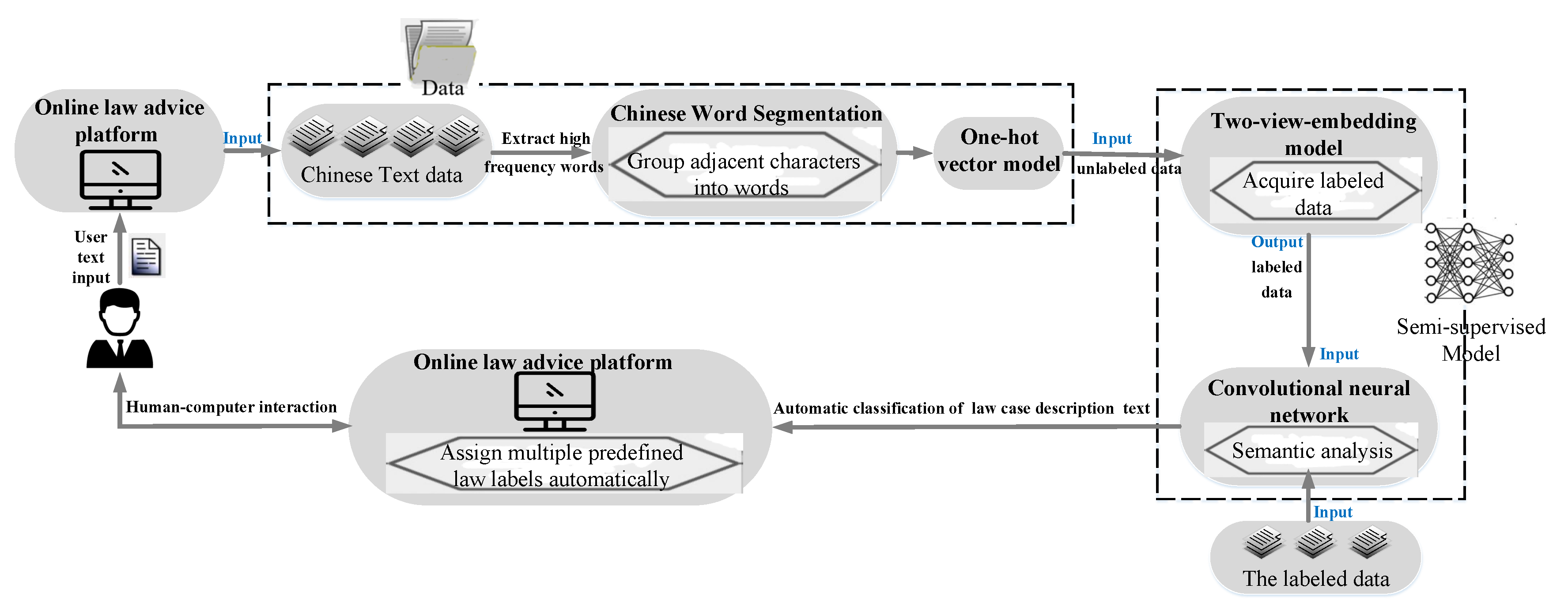
  • We propose a novel SSC-based model, with general adaptability and good scalability, to realize the Chinese text classification. Unlike English, there is no obvious division between Chinese words. To apply it to Chinese NLP tasks, firstly, a Chinese sentence needs to be segmented to get words. Then, deeper information of Chinese words is exploited to learn Chinese word vector representation. Finally, the learned word vector is integrated into the SSC model.
  • The proposed method is evaluated experimentally subject to a Chinese law case description dataset. On Chinese data, results suggest that compared to SVM, our scheme respectively improves by 7.76%, 7.86%, 9.19% and 2.96% in terms of precision, recall, F-1, and Hamming loss.
The rest of the paper is organized as follows. Section 2 presents the related work. Section 3 describes the problem of the current existing schemes to introduce the design of our scheme. We describe the implementation details of our scheme in Section 4. We evaluate the performance of our algorithm in Section 5. Finally, the paper is concluded in Section 6.

2. Related Work

In this section, the fundamentals of CNN are introduced, and then, the process is built up to understand deeply CNN applied to NLP.

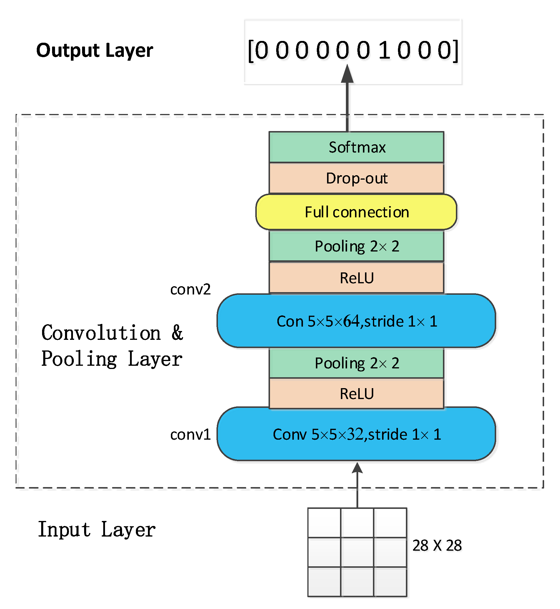
2.1. Fundamentals of CNN

CNN is a kind of feed-forward neural network that can make use of the internal structure of data. Some famous architectures have been proposed such as AlexNet [42], LeNet [43], GoogLeNet [44], VGG-16, and NiN . It is equipped with convolution layers interleaved with subsampling layers and then passes to the fully-connected layer [45]. Next, the top layer makes use of the features generated by lower layers to make the classification. Finally, the output layer exports the result, as illustrated in Figure 2. A convolution layer includes many computation units, each of which regards a region vector as the input. We apply a non-linear activation function to each vector component. The non-linear activation function may be a kind of sigmoid, tanh, rectified linear unit (ReLU) [46], and other types of activation functions. The paper uses ReLU, which is widely used at present. First of all, it is worth mentioning that CNN with ReLU trains several times faster than its equivalent with tanh.
The output of the convolution layer is the input of the subsampling layer. The subsampling layer essentially lessens the size of the input via merging neighboring regions, so that higher layers can handle more abstract and global information. A subsampling layer consists of subsampling units, each of which has a connection with a small region of the input. Average-subsampling and max-subsampling are commonly-used merging methods, which respectively calculate the channel-wise average/maximum of each region [47].
Different from most existing feed-forward networks, CNN is marked by the local connection, weight sharing, and pooling. At first, local connection reduces the number of the parameters in each layer and the model complexity [48]. Then, another distinguishing characteristic of the convolution layer is weight sharing [49], the concept of which derives from the optic nerve receptive field. Weight sharing makes the model obtain translation invariance and enhance the generalization ability. Moreover, the weight sharing operation cuts down the number of parameters as well. Finally, subsampling is another important concept of CNN. As previously mentioned, the design goal of the subsampling-based operation is to condense the adjacent region vectors of a certain size into a vector, which makes text regions narrow with a certain proportion. According to the different scaling algorithms, commonly-used scaling algorithms are the average-subsampling algorithm and the max-subsampling algorithm, which respectively calculate the channel-wise average and maximum of each region.

2.2. The Applications of CNN in NLP

Recent progress in computing power has prompted the rise of a newly-emerging technique called CNN, which has successfully been applied to image processing tasks. CNN has significant implications for image domains, but rather than being limited to image tasks, it is possible that CNN can also be applied to NLP domains. More work was done on using CNN to train text classifiers by representing natural language in a way similar to an image where each word is represented as a vector. In fact, CNN can intuitively understand words from pixels, sentences from words, and more complex concepts from sentences. The goal behind this work is to apply CNN to build models that allow an automatically-generated context-based and rich representation for the NLP task. One of the key distinctions between CNN and traditional machine learning approaches such as SVM is the ability of learning complex feature representations.
The input of NLP tasks is the sentence or the document, which is represented as a matrix [50]. Each row of the matrix corresponds to one token, typically a word, but it could also be a character. That is, each row is a vector that represents a word and a character. Typically, the vector is the word embedding such as word2vec [51], GloVe [52], and the one-hot embedding [53].
In the convolution layer for text, we represent each region (which each computation unit responds to) by a concatenation of the vectors. In the following example, there are three kinds of region sizes: 2, 4, and 6, each of which has two filters, as is shown in Figure 3. Every filter performs convolution on the sentence matrix and generates variable-length feature maps. Then one-max pooling is performed over each feature map, the maximum of which is recorded. Thus, a univariate feature vector is generated from six maps, and these six features are concatenated to form a feature vector in the penultimate layer. The final softmax layer receives this feature vector as input and uses it to classify the sentence. Here, we assume the multi-label classification task as three, so three possible output states are depicted, as is shown in Figure 3.
CNN has made great progress in NLP such as machine translation (MT), sentiment analysis, and topic assignment tasks. Benefiting from the successful application, several open-source architectures have been proposed to explore NLP [54]. Text classification can help users effectively handle and exploit useful information hidden in large-scale text. In [55], a unified framework that was based on word embedding clustering and CNN was proposed to expand short texts. Firstly, semantic cliques were discovered via fast clustering. Then, the representation of multi-scale semantic units was computed by additive composition. Next, the restricted nearest word embedding of the semantic units was chosen to constitute expanded matrices in embedding spaces. Finally, the projected matrix and expanded matrices were fed into the CNN. In [56], a series of new latent semantic models based on CNN were presented to learn the low-dimensional semantic vector from search queries and web documents.
Learning to extract semantic relations between entity pairs plays a vital role in information extraction. For relation extraction, a typical work [57] focused on the supervised framework by CNN. To obtain comparable expressivity with fewer parameters, some research [58] deeply explored an empirical study on the use of character-level CNN for text classification. Considering morphologically-rich languages, the intra-word information cannot be ignored, and the work in [59] learned character-level representation of words and associated them with usual word representations to perform POS tagging.

3. Problem Formulation and Challenges

In this section, we describe the problem of the current existing schemes. The purpose of the discussion is to make a wise decision in the design of our scheme.

3.1. Problem Description and Solutions

In recent years, the application requirement for text classification has increased dramatically. Practical text classification technology will provide convenient, natural, and effective humanized services for human–machine interaction. Benefiting from the deep learning model’s ability to learn syntactic and semantic features proactively, the human–machine interaction becomes feasible. However, for large-scale learning tasks, the supervised model applies a number of manually-designed rules and features, which come from the observations on the training set. These particular manual efforts increase the labor cost and reduce the adaptability of the learning algorithm. In this paper, the CNN framework based on the semi-supervised learning mechanism is introduced to solve the problem of data annotation and feature extraction.

3.2. Scheme

We propose an SSC framework for multi-label classification, which effectively learns the semantic information of text data. The semi-supervised model directly learns the embedding of text regions from unlabeled data with the two-view (tv)-embedding model and then integrates the learned embedding into supervised CNN. The tv-embedding model and the supervised CNN model are described in more detail in Section 4.2 and Section 4.3, respectively. The framework of the proposed model is shown in Algorithm 1.
Algorithm 1: SSC training algorithm.
Input: training data T, validation data V and test data E.
Output: the classification results R.
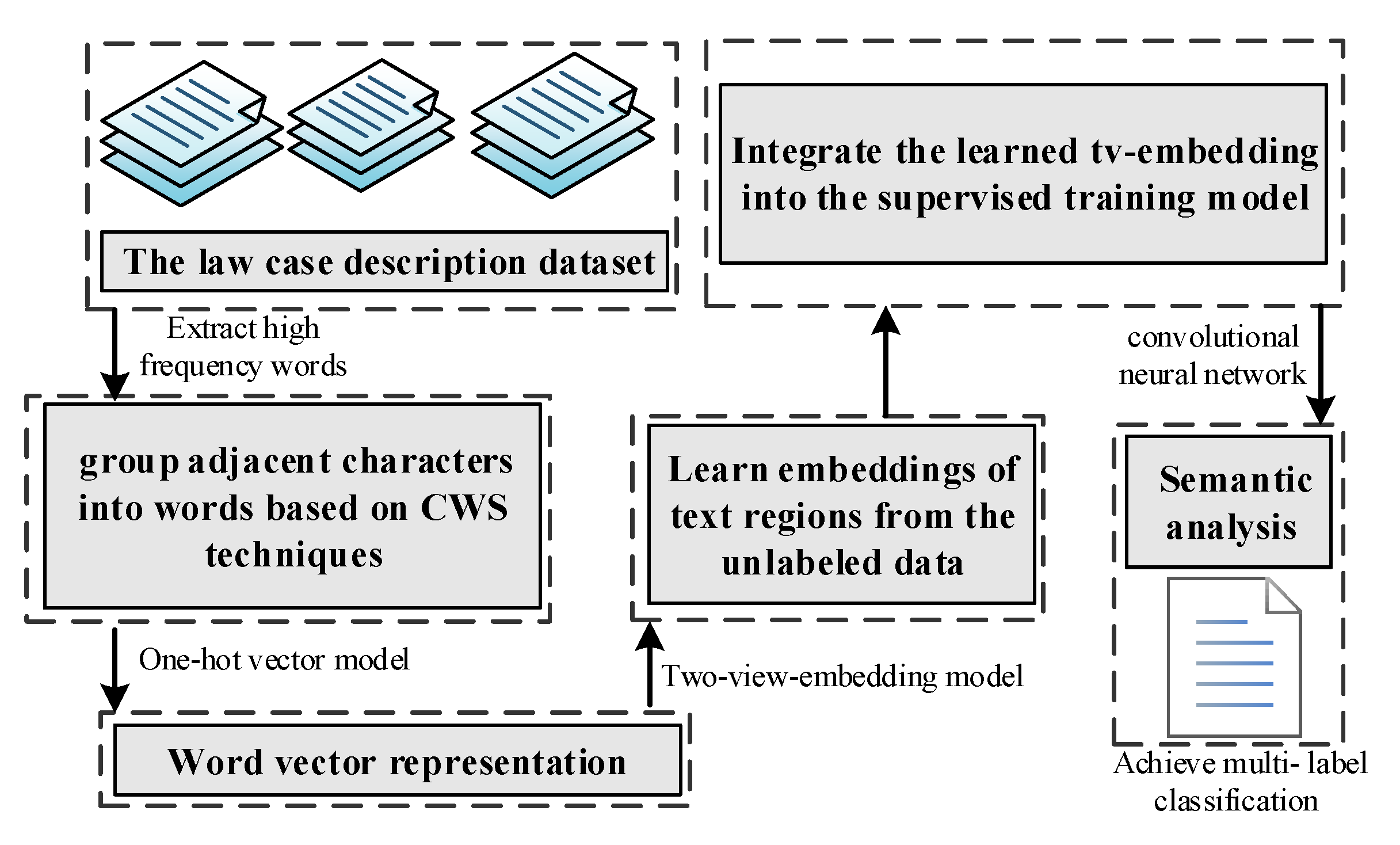
1.   extract high frequency words from the text data T;
2.   group adjacent characters into words based on the Chinese word segmentation (CWS) technique;
3.   generate the input data of the tv-embedding model by the bow-one-hot language model;
4.   train the tv-embedding model defined as P X 2 | X 1 = g 1 f 1 X 1 , X 2
        to predict adjacent regions from each small text region;
5.   set a threshold θ ;
6.   while the precision P < θ do
7.      for all convolution layers in CNN do
8.           integrate the learned tv-embedding into the CNN’s convolution layer calculated as
                 σ W · r i x + V · ν i x + b ;
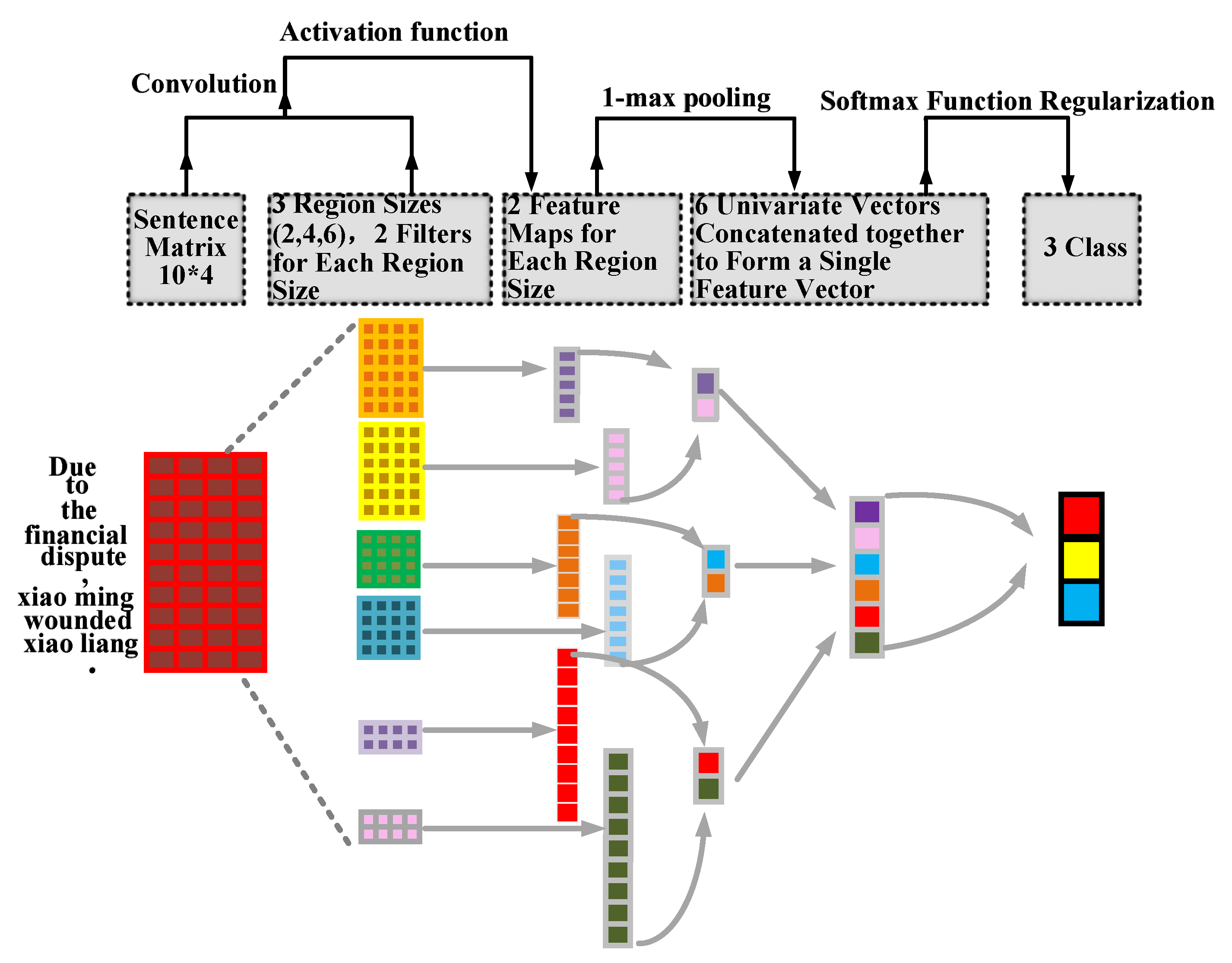
9.           the filter performs the convolution operation on the sentence matrix;
10.         get different degrees of feature dictionaries D;
11.      end for
12.      for all pooling layers in CNN do
13.         maximum pooling operation;
14.         generate a set of univariate feature vectors U;
15.      end for
16.      for softmax layer in CNN do
17.         feature vectors U are used as input to classify the text;
18.      end for
19.   return the classification results R;
20.   end while
21.   enter the validation set V, and then, adjust the classifier parameters;
22.   enter the test set E and test the classification capacity of the model.
Firstly, extract high-frequency words from dataset. For example, high-frequency words (e.g., developer, defaulted, wages, migrant workers, three years) are extracted from a legal case description: A developer has defaulted on wages to migrant workers for three years. Here, it is not necessary to use all data to implement text classification, in that keeping these input data requires much resource, leading to the waste of resources.
Secondly, based on the Chinese word segmentation (CWS) technique, adjacent characters are grouped into words.
Thirdly, generate the input data of tv-embedding learning by the bow-one-hot language model. The bow-one-hot vector is provided, which is converted from the r | V | -dimensional region vector to the | V | -dimensional vector.
Then, train the tv-embedding model to predict adjacent regions (target regions) from each small text region. The definition of tv-embedding is that if there exists a function g ( e . g . , P X 2 | X 1 = g 1 f 1 X 1 , X 2 ) , the function f 1 is the tv-embedding of χ 1 w . r . t . χ 2 for any X 1 , X 2 χ 1 × χ 2 . Given a document x, for a computation unit associated with the i th region, the convolution layer of the tv-embedding learning model calculates: ν i x = σ ν W ν · r i ν x + b ν , where σ is a predefined non-linear activation function ReLU. r i ν x is the input region vector for the i th text region. W v and b v , which are learned through training, are shared by the computation units in the same layer. The top layer uses v i x as the input vector. Note that the tv-embedding learning model is different from supervised CNN in that each small region is in contact with its own output.
Next, integrate the learned tv-embedding into the CNN’s convolution layer. The convolution layer is described using the following equations: σ W · r i x + V · ν i x + b , where ν i x is the output of the convolution layer of the tv-embedding learning model, which is associated with the i th region. We update the weight matrix W, V, bias vector b, and the top-layer parameters.
Again, train the supervised CNN model.
After that, enter the validation set, and then, adjust the classifier parameters. The function of validation set is to evaluate the single evaluation index (e.g., accuracy, precision, or recall rate). Through this evaluation index, the algorithm parameters can be adjusted by comparing the training set with the validation set. For example, if the recall rate of the training set is 0.9 and the recall rate of the validation set is 0.6, we may have an overfitting situation. In order to reduce fitting, the number of iterations needs to be reduced or L 2 regulars need to be set.
Finally, enter the test set, and test the classification capacity of the model.

3.3. Challenges

In a nutshell, data annotation and feature extraction are two very important issues in text classification. Based on CNN theory, two main technical challenges should be considered to improve the classification precision and speed up the classification performance. We conclude the challenges as the following aspects:
  • For large-scale learning tasks in NLP, the training data need to be manually annotated, which increases the labor and time costs and tremendously limits the general adaptability of NLP.
  • It is important to note that while the CNN-based online law consulting system has achieved better intelligent experience than other studies, significant challenges remain on the internal structure of the model, such as fewer network layers to extract text feature.
Note that a refined vector representation of the law data is a prerequisite for dealing with a mass of law cases urgently and classifying the law text automatically. Before we improve the model performance, we first realize the refined vector representation of law data and the full extraction of feature information in order to implement text classification accurately.

4. The Implementation of Our Scheme

In this section, we will describe the implementation details of our scheme. Firstly, extract high-frequency words from the law case description document. Secondly, based on the Chinese word segmentation (CWS) techniques, adjacent characters are grouped into words. Thirdly, generate the input data of tv-embedding learning by the one-hot language model. Then, train the tv-embedding model to learn the embedding of text regions from unlabeled data. Finally, integrate the learned label embedding into the CNN’s convolution layer. In this section, we mainly describe the one-hot language model, the tv-embedding model, and the supervised CNN.

4.1. One-Hot Embedding for Small Text Regions

The CNN-based model is a kind of DNN framework, which can use the internal structure of the data. In this paper, we study CNN on text processing to use the 1D structure (namely, word order) of text data for the effective semantic analysis task. We directly learn vector representations of the high-dimensional text regions to obtain the predictive ability of co-present and absent words in the classification task. In contrast, a low-dimensional word vector is trained to only represent individual words in isolation. In this sense, a text region can be more expressive than the simple average of word vectors in isolation.
In practical application, the feature values are not always continuous values. Sometimes, they are classified values (namely, discrete values) such as gender characteristics, which can be divided into boys and girls. In machine learning, such feature information is usually digitized. In this paper, we introduce the one-hot vector model to implement effective mathematical representation for the discrete values.
For text classification, one-hot CNN has been successfully applied, as illustrated in Figure 4, where it applies CNN to high-dimensional one-hot vectors directly and learns directly the embedding of small text regions [53]. Now, we consider the application of one-hot embedding to text data. Suppose that the text description of a law case L with vocabulary V, which is represented by L = τ 1 , τ 2 , · · · , τ n , is given. For text, a straightforward representation would be to treat each word as a pixel and the entire sentence as an image, which is L × 1 pixels with V channels. The goal here is to represent each word as a | V | -dimensional one-hot vector. For example, suppose that vocabulary V = a , developers , default , migrant , pay , time , on , workers , wages , which is in alphabetical order, and that the text description of a law case L = (Developers default on migrant workers’ wages). Then, we have a one-hot-vector: t = 010000000 001000000 000000100 000100000 000000010 000000001 .
Next, we introduce the seq-one-hot-vector (“seq” for keeping sequences of words) and bow-one-hot-vector. For text representation, each text region is represented by a concatenation of the pixels (namely, each word). Each region, which each computation unit responds to, makes r | V | -dimensional region vectors where r is the region size fixed in advance. For example, on the example text vector t above, with r = 3 and s t r i d e = 2 , we would have three regions “developers default on”, “on migrant workers”’, and “workers’ wages”, represented by the following seq-one-hot-vector: r 0 t = 010000000 001000000 000000100 , r 1 t = 000000100 000100000 000000010 , r 2 t = 000000010 000000001 000000000 . However, a potential problem of the seq-one-hot-vector method is that the dimensionality of each region vector r i t could be very high if the number of the vocabulary V is very large. Therefore, it raises the urgency of considering other alternatives to the word vector representation. Here, an alternative is provided to perform the bow-one-hot-vector, which is converted from the r | V | -dimensional region vector to the | V | -dimensional vector. For example, the seq-one-hot-vector above would be converted to: r 0 t = 011000100 , r 1 t = 000100110 , r 2 t = 000000011 . With bow-one-hot-vector representation, fewer parameters are learned. In this paper, we use the bow-one-hot vector representation to alleviate the problem of high-dimensional data and solve the problem caused by the discrete values.

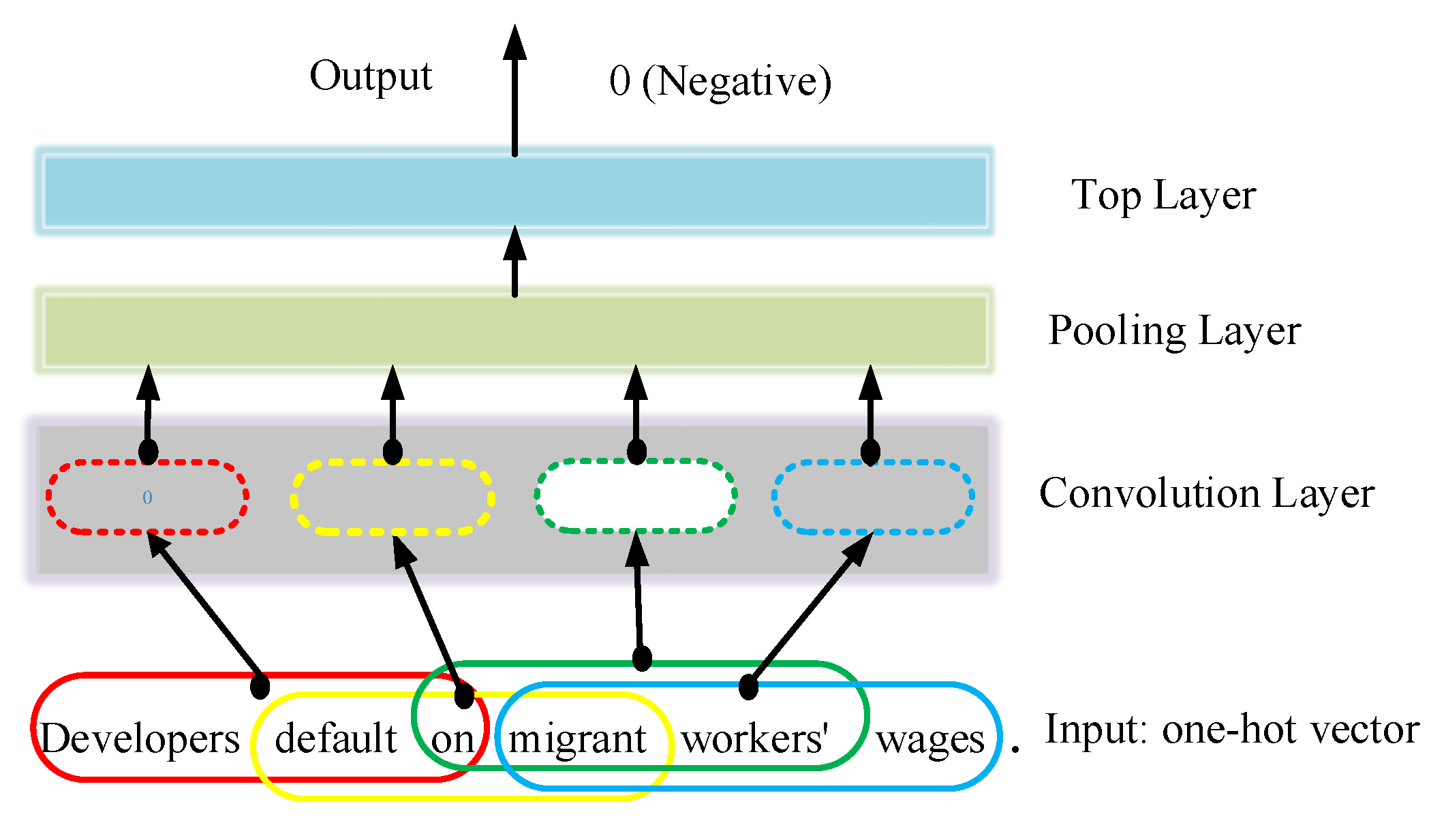
4.2. tv-Embedding Model

The semi-supervised learning framework includes the following two steps: tv-embedding (tv represents two-view) learning and supervised learning. Semi-supervised model directly learns the embedding of text regions from unlabeled data with the tv-embedding learning model and then integrates the learned embedding into supervised CNN. The learned embedding regions (the output of the tv-embedding learning model) are used as the additional input to the supervised model.
The first step of the semi-supervised learning model is to learn the region embedding from no-label text data, as illustrated in Figure 5. The definition of tv-embedding is that if there exists a function g ( e . g . , P X 2 | X 1 = g 1 f 1 X 1 , X 2 ) , the function f 1 is the tv-embedding of χ 1 w . r . t . χ 2 for any X 1 , X 2 χ 1 × χ 2 . A tv-embedding of a view (X1) keeps the required structure in order to generate another view (X2), which learns useful feature vectors from no-label text data. For the tv-embedding learning model, a neural network is trained to predict the adjacent regions from each small text region. That is, convolution layers produce useful feature vectors from each small text region. Then, the classifier in the top layer uses the feature vectors. Since each small text region is associated with its own output, the tv-embedding model has a distinguishing difference from CNN. We conclude the goals that the tv-embedding model mainly implements as the following aspects:
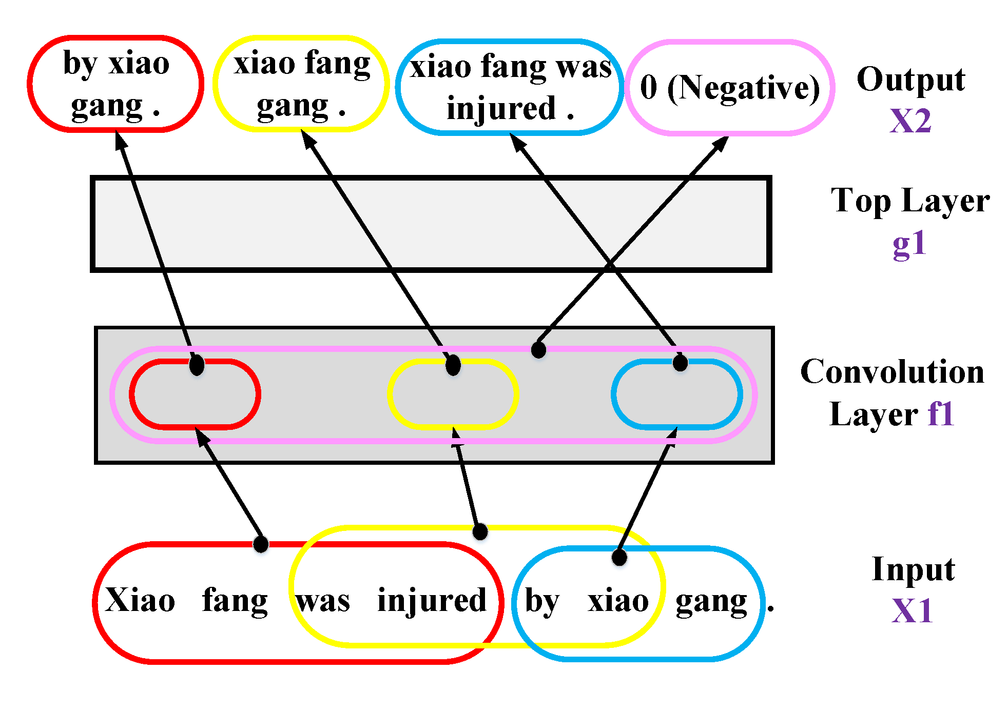
  • It implements the goal to predict the adjacent text region from each region of size p. What is more, it can capture the internal information between data.
  • It can assign a sub-label (e.g., positive/negative) to each small text region of size p. For example, in Figure 5 above, with p = 4 and s t r i d e = 2 , three regions “Xiao fang was injured”, “was injured by Xiao” and “by X Xiao gang” are assigned sub-labels 0, 0, 1, respectively. Note that 1 means positive, 0 means negative. It is worth noting that assigning a sub-label to each small text region of size p is sensible because these small text regions are helpful for making classification.
  • It also assigns a total label (e.g., positive/negative) for the entire sentence. For example, the entire sentence “Xiao fang was injured by Xiao gang.” is assigned a total label 0, as illustrated in Figure 5. Note that 1 means positive, 0 means negative. This is sensible because CNN makes classification by analyzing the entire sentence as well.
  • A convolution layer learns the embedding of small regions from no-label text data. The high-dimensional feature vectors are converted to the low-dimensional feature vectors; in addition, the predictive structure is preserved.
Given a document x, for a computation unit associated with the i-th region, the convolution layer of the tv-embedding learning model calculates:
ν i x = σ ν W ν · r i ν x + b ν
where σ is a predefined non-linear activation function ReLU (namely, f x = max 0 , x ), which is applied to each vector component. r i ν x is the input region vector for the i-th text region, which can be either the seq-one-hot-vector, the bow-one-hot vector, or the bag-of-n-gram. In this paper, we use the bow-one-hot vector, which solves the problem of high-dimensional data. W v and b v , which are learned through training, are shared by the computation units in the same layer. The top layer uses v i x as the input vector. The goal here is to learn a vector representation of the small text region and assign a sub-label (e.g., positive/negative) to each small text region and a total label (e.g., positive/negative) for the entire sentence. It is worth mentioning that the convolution layer embodies the tv-embedding. We transfer to the supervised learning model in the next step.

4.3. Integration of the tv-Embedding into Supervised CNN

The second step of the semi-supervised model is the integration of the tv-embedding region into supervised CNN, that is the tv-embedding feature from no-label data is regarded as the additional input to the convolution layer of CNN model. We compute the computation unit of the CNN’s convolution layer by replacing σ W · r i x + b with:
σ W · r i x + V · ν i x + b
where ν i x is defined by Equation (1), that is ν i x is the output of the convolution layer of the tv-embedding learning model, which is associated with the i-th region. We update the weight matrix W, V, bias vector b, and the top-layer parameters, so that we minimize the designated loss function on the labeled data. Seen from the above Formula (2), the learned tv-embedding regions are used as an additional input to the CNN’s convolution layer to solve the data annotation problem.
The output of the convolution layer is put into the pooling layer, which is a no-parameter layer. The essence of the pooling layer is to shrink the data size by merging the neighboring region. That is, it brings down the dimension of the data. Therefore, a higher layer can process more abstract (namely, more global) information. The reason why it does is that more abstract feature information can fully represent data, even if it reduces much feature information. Due to decreasing the dimension of the data, it can avoid overfitting as well. Frequently-used merging methods are average-pooling and max-pooling in the pooling layer. A pooling layer includes a number of pooling units, where each of pooling unit responds to a small region of text data.

5. Performance Evaluation

With the rapid development of artificial intelligence technology, it is very intuitive to realize the human–machine interaction based on NLP. The system deals with a mass of law cases and classifies the law text, which automatically recognizes and assigns the predefined law label. The system can carry out online law advice, law case handling, and other services, which greatly reduces the workload of lawyers, while bringing convenience for people who lack law knowledge. Figure 6 shows the frame diagram of the automatic classification of law text.

5.1. The Experiment Platform

In this paper, the construction and training of CNN are realized in the following experimental configuration. The experimental platform was installed on a 64-bit Ubuntu 14.04 system, and the training was run in the Python environment. Configure the deep learning toolkit, firstly, and update the environment and gcc . Secondly, build the Python running environment. Thirdly, install the math tools: numpy, scipy, and theano. Then, install a theano-based deep learning package called pylearn2. Next, install the DNN scikit-neuralnetwork. Again, install the Python test tool nose and some dependent packages (such as libpng-dev, libjpeg-dev, and libfreetype6-dev). Finally, initialize the display environment. The experimental configuration is shown in Table 1.

5.2. Dataset

The law case description dataset, which was collected by relevant scholars, was derived from Find Law Network (http://china.findlaw.cn/) and China Law Document Network (http://www.falvwenshuwang.com/), and we regarded it as the corpus to conduct the experiments. Aiming to conduct comparative experiments, we introduced the English standard dataset RCV1 . Although the English standard dataset RCV1 is a corpus of Reuters news articles described in LYRL04 [60], it can be used to verify the performance of the proposed model. RCV1 includes 103 topic classifications, which belong to multi-label classification. In multi-label classification tasks, RCV1 shows good performance [61,62]. Apart from Chinese word segmentation (CWS) techniques, all other techniques in Algorithm 1 were applied to the English standard dataset RCV1.
The Chinese law case description dataset was regarded as the corpus to evaluate the model performance. The Chinese law case description dataset was associated with more than one law label, which belonged to multi-label classification. That is, a law case description text was entered into the law advice system, which was processed by the system, and then, multiple predefined law labels were recognized and assigned automatically that matched the event description. On the multi-label classification of 25 law categories, the entire corpus was divided into 16,000 items for the training set, 2000 items for the validation set, and 2000 items for the test set, as shown in Table 2. To use as unlabeled data, we chose 500 K law texts from the same data source, so that they were disjoint from the training set, validation set, and test set. There are many law categories in China. In this paper, we mainly deal with 25 categories including constitution, economic law, financial tax law, criminal law, medical law, road traffic law, civil law, ocean law, real estate and construction law, administrative law, labor law, civil service law, anti-corruption law, intellectual property law, individual income tax law, environmental law, press and publication law, judicial procedure law, labor education law, cultural relics protection law, radio and television policy law, tobacco law, religious law, industrial and commercial administration law, and information technology law. We set these 25 law categories as labels. Through the treatment of the law case description, infringed victim’s rights or laws violated by the parties were initially confirmed. We noted that multiple rights of a victim may be violated or a party may violate multiple laws at the same time. For example, the party enters a law case description into the system, and after processing the system, a number of predefined legal labels such as economic law and financial tax law are output. That is to say, the party violated both economic law and financial tax law. The law advice system brings convenience for people who lack law knowledge. For preprocessing, firstly, we extracted high-frequency words from input data; secondly, adjacent characters were grouped into words based on Chinese word segmentation (CWS) techniques; thirdly, words were represented as vectors by the one-hot model.
For the multi-label classification of 103 topics on RCV1, since the official LYRL04 split for this task divided the entire corpus into a training set and a test set, the entire test set was used as unlabeled data, as shown in Table 2. Performance on the multi-label classification task was sensitive to thresholding strategies. As described in [60], the concatenation of the headline and text elements was used. For preprocessing, all the characters were converted to lower case. Moreover, the stop word list, which was provided by LYRL04, were used, and numbers were regarded as stop words.

5.3. Evaluation of the Classification Performance

The performance of text classification depends of the use of the loss function (e.g., square, log, and BinLogi2) to assess the evaluation. In the multi-label classification task, the paper uses the BinLogi2 to assess the classification evaluation. BinLogi2 is the logistic loss function, which is defined as L θ i = i = 1 m log 1 + exp 2 y 1 p θ i where p θ i is the prediction value and y is the target value. The loss function forms a curved surface, and here, our goal is to find the lowest point of the curved surface. Moreover, the gradient descent algorithm can work out the minimization problem of the loss function. Suppose that we stand on a point of a curved surface and our goal is to arrive at the lowest point with the fastest speed. Without doubt, we walk down along the largest direction of the gradient (namely, the opposite direction of the gradient) to reach the lowest point. The gradient descent algorithm was used to update the parameters (namely, W and b) continuously to obtain the minimum value of the loss function. In other words, the partial derivative of the shared weight W and the bias term b were calculated by the loss function, and then, the weight and the bias term were updated.
This is the process taking the partial derivatives with mathematical description:
θ i L θ i = θ i i = 1 m log 1 + exp 2 y 1 p θ i
where L θ i is the loss function, p θ i is the predicted value, and y is the target value.
The update process of the parameters (e.g., weight W and bias b) is defined as follows:
ω k = ω k η L ω k
b l = b l η L b l
where ω k is the weight applied to the k-th computation unit, ω k is the partial derivatives of ω k , b l is the bias associated with the l-th computation unit, b l is the partial derivatives of b l , η is the learning rate, L ω k shows that the loss function calculates the partial derivative for weight, and L b l is shows that the loss function calculates the partial derivative for the bias.
The gradient descent algorithm uses all instances each time, so it has difficulties improving the training speed and shortening the training time. To solve the problem of slow training, the stochastic gradient descent (SGD) algorithm is proposed. Suppose that a dataset including 1000 training instances is given, which is disturbed randomly, and then divided into a number of small pieces on the average. Each time, we take a small sample (namely, a mini-batch) from all the training examples to make training up to using all instances, and we call it an epoch. Therefore, training the neural network using mini-batch SGD can help us to improve the learning rate. The SGD algorithm is given as follows:
ω k = ω k η m j L X j ω k
b l = b l η m j L X j b l
where ω k is the weight after the update applied to the k-th computation unit, ω k is the weight before the update associated with the computation unit k-th, η is the learning rate, m is the size of each mini-batch, and L X j ω k is the loss function L, which calculates the partial derivative for weight ω , as illustrated in Equation (6). Analogously, the bias b l is also updated to b l , as illustrated in Equation (7).

5.4. Experimental Results

In this section, we conduct experiments using different internal structures which are different numbers of hidden layers, different numbers of neurons, and different region sizes (e.g., region size of two, region size of three, and so on). Besides comparing the performance of different internal structures, we also discuss the impacts on different kinds of languages. Extensive experiments confirm that our method not only improves the precision, but also speeds up classification performance greatly.

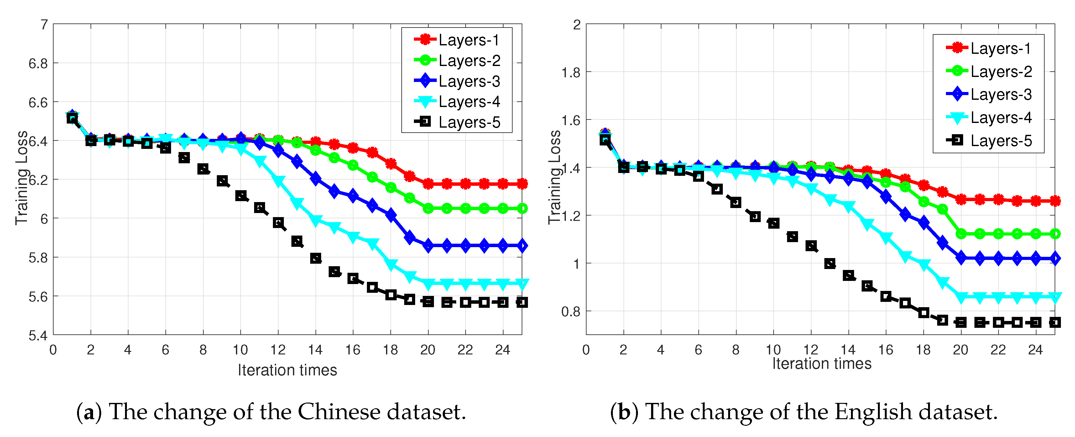
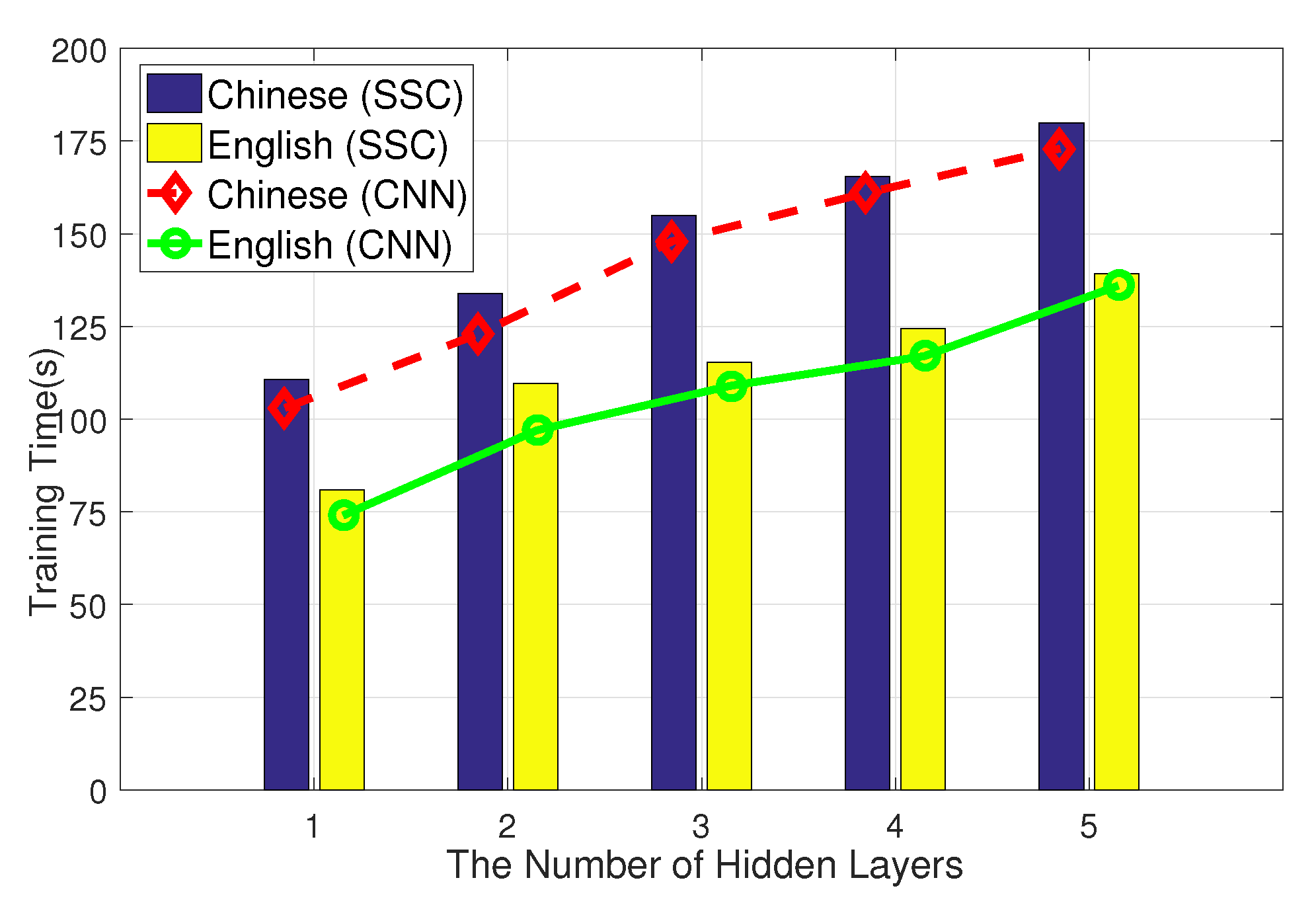
5.4.1. Depth Improves Performance

As shown in Figure 7, the horizontal and vertical coordinates represent the iteration times and the training loss rate (%), respectively. We found that the network depth improved the model performance, that is the training loss rate of the model would decrease as the number of hidden layers increased within a certain range. The reason is that more hidden layers can fully extract feature information for use in the classifier of the top layer. Increasing the model depth from 1one to five on the English dataset (namely, RCV1) and the Chinese dataset (namely, the Chinese law case description), the training loss rate was approximately reduced by 0.5% and 0.6%, respectively, as shown in Figure 7. Compared with Figure 7a, Figure 7b has less training loss. On the same hidden layers, comparing with the training loss rate of the Chinese dataset, the training loss rate of the English standard dataset was approximately decreased by 4.85 %. The reason is that unlike English, there is no obvious division between Chinese words. Thus, it was more difficult to deal with Chinese text than English text. From the results, firstly, the more the number of hidden layers there were, the smaller the training loss was. Secondly, with the same number of hidden layer, the training loss was smaller and smaller following the iterations. Thirdly, the performance of Chinese text was worse than that of English text on the same network configuration.

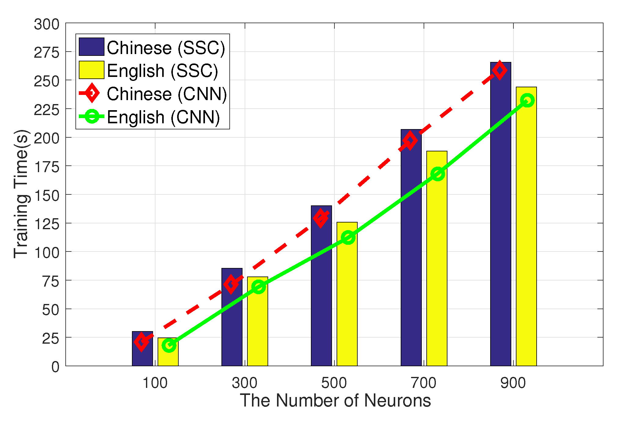
5.4.2. Neurons Improve Performance

We compared the influence of the number of neurons on the model performance, as shown in Figure 8. The results indicated that as the number of neurons in the hidden layer increased, the training loss rate of the model decreased. In other words, the number of neurons improved the semantic analysis performance. Increasing the number of neurons from 100 to 900 on the English dataset and the Chinese dataset, the training loss rate was approximately reduced by 0.2% and 0.3%, respectively. Compared with Figure 8b, Figure 8a has a greater training loss rate. Compared with the training loss rate of the Chinese dataset, the training loss rate of the English standard dataset was approximately decreased by 5.25 % on 900 neurons. The reason is that unlike English, there is no obvious division between Chinese words. Thus, it was more difficult to deal with Chinese text than English text. The first thing to note is that the more the number of neurons there was, the smaller the training loss was, which confirmed the effectiveness of the model we proposed. It also plotted the loss rate with respect to the iteration times, which indicated that more iteration times had an advantage of smaller loss in the case of the same neurons.

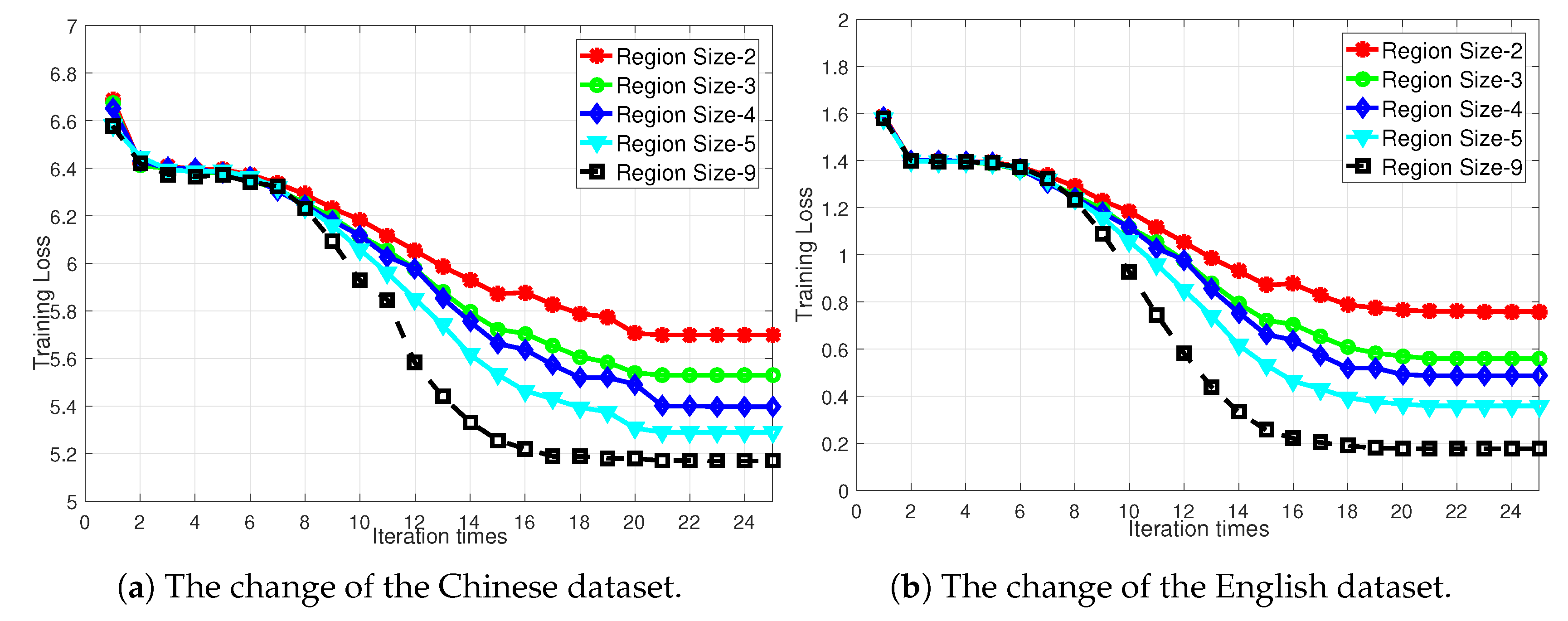
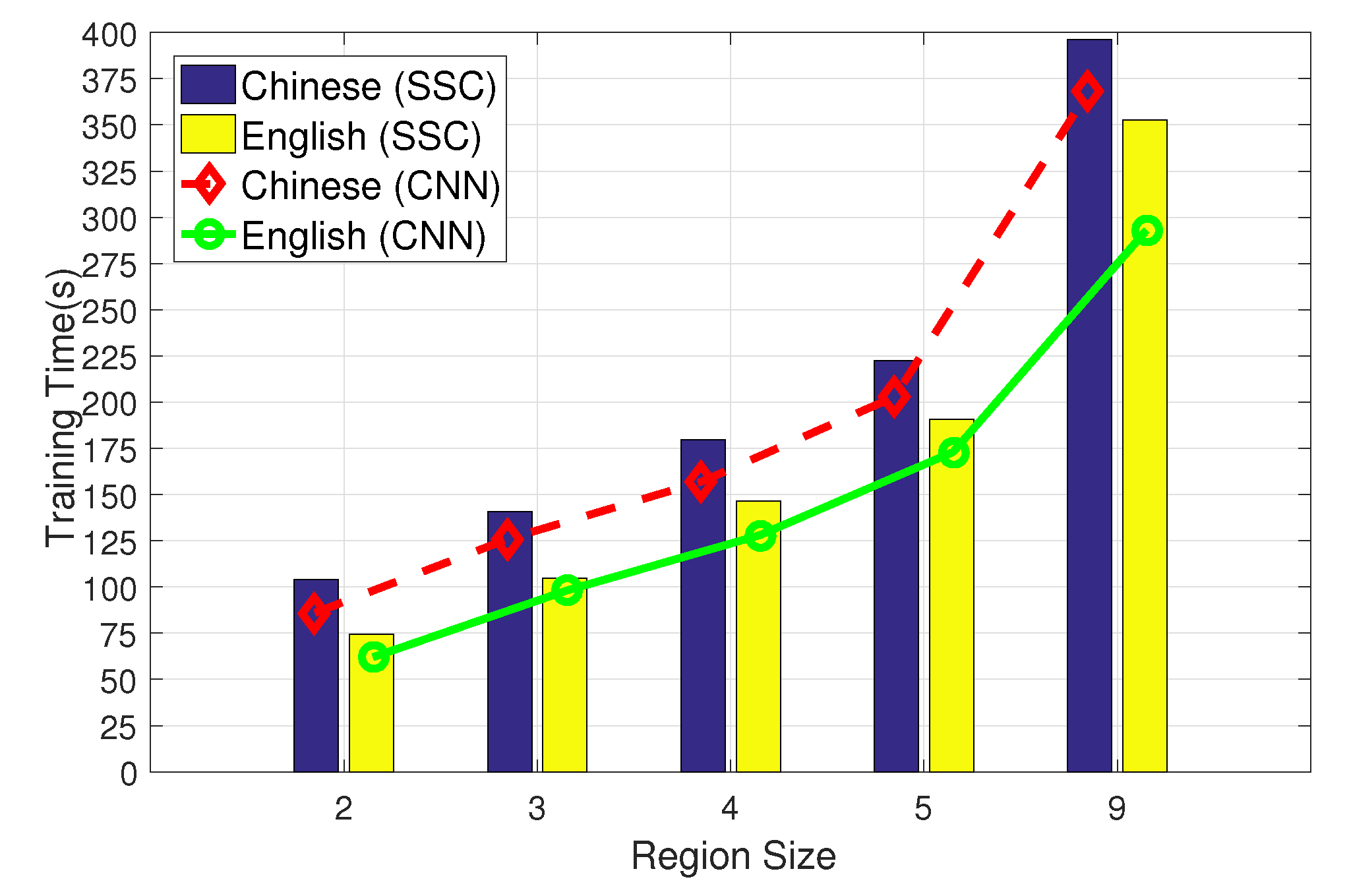
5.4.3. Bigger Region Size Improves Performance

We found that the number of the region size in the same convolution layer had an impact on the model performance, as illustrated in Figure 9. This indicated that feature extraction was carried out simultaneously on the same convolutional layer with multiple region sizes of different dimensions. Increasing the region size from 2 to 9 on the English dataset and the Chinese dataset, the training loss rate was approximately reduced by 0.6% and 0.5%, respectively. Besides comparing the performance of different types of region sizes, it is of interest to compare the performance of different iteration times on the same region size. Note that, as the iteration times increased, the training loss rate decreased. Compared with Figure 9a, Figure 9b has less training loss. for the same region size, compared with the training loss of the Chinese dataset, the training loss of the English standard dataset was approximately decreased by 5.01%. The reason is that unlike English, there is no obvious division between Chinese words. Thus, it was more difficult to deal with Chinese text than English text.

5.4.4. Comparison of Different Datasets

Besides comparing the performance of different internal structures, we also conducted experiments on different nature languages: English dataset (namely, RCV1) and Chinese dataset (namely, the Chinese law case description). There is a massive gap between Chinese and English. Distinguished from English, there is no obvious division between Chinese words. In addition, Chinese still suffers from the sparseness of data, and rare words question whether it is on the sentence level or word level.
We experimented with the same network configurations (namely, the same number of hidden layers, the same number of neurons, the same region size, and so on). On multi-label text classification, the training loss of the Chinese law case description was slightly higher than that of the English standard dataset, as shown in Figure 10. The reason is that unlike English, there is no obvious division between Chinese words. Thus, it was more difficult to deal with Chinese text than English text. That is, the performance of Chinese text is worse than that of English text on the same model.

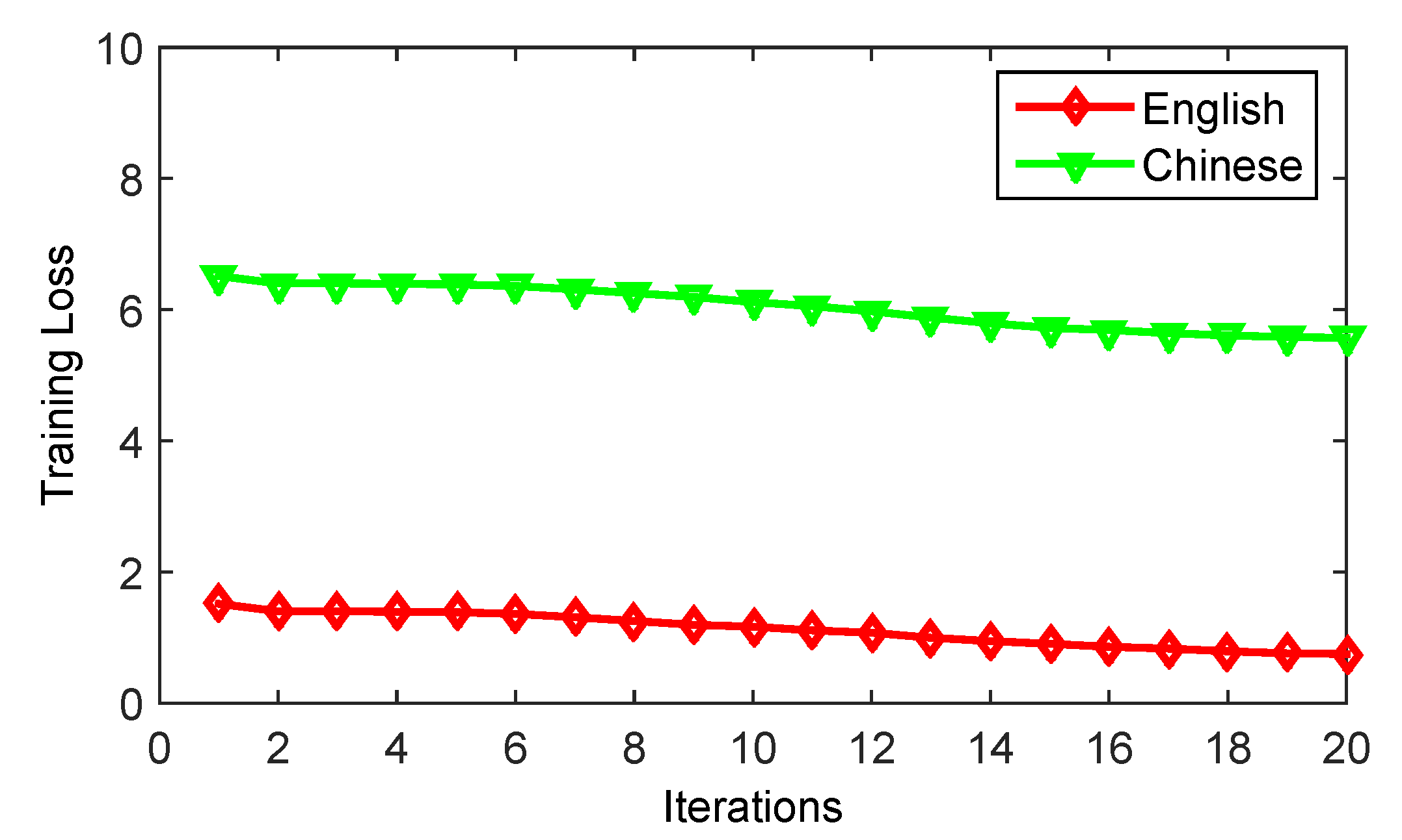
5.4.5. Comparison of Time Consumption

Figure 11 shows the relation between the training time and the number of hidden layers in which the horizontal and vertical coordinates represent the number of hidden layers and the training time, respectively. The training time is known to increase following the number of hidden layers. The reason is that as the number of hidden layers increased, the model became more and more complex, so that more time was needed for training. In addition, we compared our model with CNN [53]. Note that, even though two different kinds of methods (SSC and CNN) were trained, the changing law was similar. As shown in Figure 11, the training time of SSC was more than that of CNN. Moreover, the training time of the Chinese dataset was more than that of the English dataset. The reason is that unlike English text, there are no spaces between Chinese characters. Based on Chinese word segmentation (CWS) techniques, a Chinese sentence needs to be segmented to get words. Thus, it takes more time to process Chinese text.
Moreover, we compared the influence of the number of neurons on the training time, as shown in Figure 12. The horizontal and vertical coordinates represent the number of neurons and the training time, respectively. As can be seen from Figure 12, as the number of neurons increased, the training time was more and more. The reason is that, as the number of neuron increased, the model became more and more complex, so that more time was needed for training. In addition, we compared our method with CNN. The results demonstrated that the training time of our scheme was more than that of CNN. Analogously, since there are no spaces between Chinese characters, it was more difficult to deal with the Chinese text. Thus, the training time of Chinese dataset was more than that of the English dataset, as shown in Figure 12.
Besides, we compared the change of training time with respect to different region sizes. Figure 13 shows that with the augmentation of region size, the training time was more and more. The reason is that as the region size was bigger and bigger, the model became more and more complex, so that more time was needed for training. The results also demonstrated that compared with CNN, our scheme needed to take more time to train the model. As can be seen from Figure 13, the changing law of the English dataset was similar to the Chinese dataset, but the training time of the Chinese dataset was more than that of the English dataset. Similarly, since there are no spaces between Chinese characters, it was more difficult to deal with the Chinese text.

5.4.6. Performance Results of Different Models

Table 3 shows the evaluation of the classifier’s performance. As shown in Table 3, the first row is the linear SVM algorithm for multi-class text classification [63]; the second row is the CNN [53] model; the third row is the semi-supervised model [25]; and the last row is the SSC model.
The first thing to note is that the best-performing SSC outperformed the baseline methods on all datasets, which demonstrated the effectiveness of our model. After affirming the effectiveness of our model in comparison with the SVM, CNN, and the semi-supervised model, Table 3 summarizes the experimental results of different methods. As shown in Table 3, the experimental results demonstrated that the precision, recall, and F-1 score of the English dataset (namely, RCV1) were slightly higher than the Chinese law case description dataset on all models. The reason is that, there is a massive gap between Chinese and English. Distinguished from English, there is no obvious division between Chinese words. In addition, Chinese still suffers from the sparseness of data, and rare words question whether it is on the word level or character level. Thus, it was more difficult to deal with the Chinese text than the English text. That is, the performance of the Chinese text was worse than that of the English text on the same model. We compared our method with some state-of-the-art machine learning methods. On the Chinese law case description dataset, the best precision 95.48%, the best recall 91.98%, the best F-1 93.78%, and the best Hamming loss were obtained by SSC. On the Chinese data, the simulation results demonstrated that in terms of precision, recall, F-1, and Hamming loss, our scheme respectively improved them by 7.76%, 7.86%, 9.19%, and 2.96% compared with the linear SVM. Analogously, the simulation results demonstrated that, compared with CNN, our scheme respectively improved by 4.46%, 5.76%, 5.14%, and 0.87% the precision, recall, F-1, and Hamming loss.

6. Conclusions and Future Work

A decision support online law consulting platform is necessary to automatically recognize and assign predefined law labels, which greatly reduces the workload of lawyers, while bringing convenience for people who lack law knowledge. In this paper, we proposed a new SSC algorithm for Chinese law text classification. Unlike English, there is no obvious division between Chinese words. Based on the Chinese word segmentation (CWS) techniques, adjacent characters were grouped into words in order to apply to the Chinese text classification tasks. Our method learned the embedding of small text regions from unlabeled data and then integrated the learned embedding into the supervised training. More specifically, the learned embedding regions with the two-view-embedding model were used as an additional input to the CNN’s convolution layer to solve the problem of data annotation. In addition, to implement the multi-task learning, a multi-label classification algorithm was proposed, which assigned multiple categories to an instance. We conducted extensive experiments over a real dataset and compared our method with some state-of-the-art machine learning methods. On the Chinese data, the results suggested that in terms of precision, recall, F-1, and Hamming loss, our method respectively improved them by 7.76%, 7.86%, 9.19%, and 2.96% compared with the linear SVM. Moreover, compared to CNN, our method respectively improved by 4.46%, 5.76%, 5.14%, and 0.87% the precision, recall, F-1, and Hamming loss. It is worth mentioning that the robustness of this method made it suitable and effective for automatic classification of law text. Furthermore, the design concept proposed is promising, which can be utilized in other real-world applications such as news classification and public opinion monitoring. However, there is still much work left to do. The extent to which this type of model can be scaled to much larger and wider domains remains an open question that we hope to pursue in our further work.

Author Contributions

All authors contributed equally to this work. F.Z. and P.L. conceived and designed the experimental scheme; F.Z. and Y.L. (Yuanyuan Li) performed the experiments; J.H. and Y.L. (Yinguo Li) contributed data analysis; F.Z. and P.L. wrote the paper.

Funding

This research was funded by Ministry of Education - China Mobile Research Fund MCM20180404; Chongqing Basic Research and Frontier Exploration Project cstc 2018jcyjAX0167; Chongqing Artificial Intelligence Technology Innovation Major Theme Special Project cstc 2017 rgzn-zdyfX0035; Chongqing Key Industries Common Key Technological Innovation Specialized cstc 2017zdcy-zdyfX0067.

Conflicts of Interest

The authors declare no conflict of interest.

References

  1. Kirkpatrick, K. Legal advice on the smartphone. Commun. ACM 2016, 59, 19–21. [Google Scholar] [CrossRef]
  2. Jing, L. Platform Economy in Legal Profession: An Empirical Study on Online Legal Service Providers in China. Soc. Sci. Electron. Publ. 2018, 35, 97–153. [Google Scholar]
  3. Peressutti, D.; Sinclair, M.; Bai, W.; Jackson, T.; Ruijsink, J.; Nordsletten, D.; Asner, L.; Hadjicharalambous, M.; Rinaldi, C.A.; Rueckert, D. A Framework for Combining a Motion Atlas with Non-Motion Information to Learn Clinically Useful Biomarkers: Application to Cardiac Resynchronisation Therapy Response Prediction. Med. Image Anal. 2017, 35, 669–684. [Google Scholar] [CrossRef] [PubMed]
  4. Wu, Z.; Zhu, H.; Li, G.; Cui, Z.; Huang, H.; Li, J.; Chen, E.; Xu, G. An efficient Wikipedia semantic matching approach to text document classification. Inf. Sci. 2017, 393, 15–28. [Google Scholar] [CrossRef]
  5. Eger, S.; Youssef, P.; Gurevych, I. Is it time to swish? comparing deep learning activation functions across NLP tasks. arXiv 2019, arXiv:1901.02671. [Google Scholar]
  6. Yamada, I.; Ito, T.; Takeda, H.; Takefuji, Y. Linkify: Enhancing Text Reading Experience by Detecting and Linking Helpful Entities to Users. IEEE Intell. Syst. 2019, 33, 37–46. [Google Scholar] [CrossRef]
  7. Kurita, S.; Kawahara, D.; Kurohash, S. Neural Adversarial Training for Semi-supervised Japanese Predicate-argument Structure Analysis. arXiv 2018, arXiv:1806.00971. [Google Scholar]
  8. Young, T.; Hazarika, D.; Poria, S.; Cambria, E. Recent Trends in Deep Learning Based Natural Language Processing. IEEE Comput. Intell. Mag. 2017, 13, 55–75. [Google Scholar] [CrossRef]
  9. Desmet, B.; Hoste, V. Online suicide prevention through optimised text classification. Inf. Sci. 2018, 439–440, 61–78. [Google Scholar] [CrossRef]
  10. Baolin, W.; Tom, A.; David, F.; Walter, M.M.; Gil, M.; Kathryn, S.; David, W.; Kenneth, W.; Hongyu, Z. Comparison of statistical methods for classification of ovarian cancer using mass spectrometry data. Bioinformatics 2003, 19, 1636–1643. [Google Scholar] [Green Version]
  11. Brodeur, J.; Coetzee, S.; Danko, D.; Garcia, S.; Hjelmager, J. Geographic Information Metadata—An Outlook from the International Standardization Perspective. ISPRS Int. J. Geo-Inf. 2019, 8, 280. [Google Scholar] [CrossRef]
  12. Mehmood, A.; Jia, S.; Mahmood, R.; Yan, J.; Ahsan, M. Non-Stationary Bayesian Modeling of Annual Maximum Floods in a Changing Environment and Implications for Flood Management in the Kabul River Basin, Pakistan. Water 2019, 11, 1246. [Google Scholar] [CrossRef]
  13. Guyon, I.; Weston, J.; Barnhill, S.; Vapnik, V. Gene Selection for Cancer Classification using Support Vector Machines. Mach. Learn. 2002, 46, 389–422. [Google Scholar] [CrossRef]
  14. Sun, D.; Zhu, Y.; Xu, H.; He, Y.; Cen, H. Time-Series Chlorophyll Fluorescence Imaging Reveals Dynamic Photosynthetic Fingerprints of sos Mutants to Drought Stress. Sensors 2019, 19, 2649. [Google Scholar] [CrossRef] [PubMed]
  15. Hsu, C.N.; Huang, H.J.; Wong, T.T. Implications of the Dirichlet assumption for discretization of continuous variables in naive Bayesian classifiers. Mach. Learn. 2003, 53, 235–263. [Google Scholar] [CrossRef]
  16. Chen, W.J.; Shao, Y.H.; Li, C.N.; Deng, N.Y. MLTSVM: a novel twin support vector machine to multi-label learning. Pattern Recognit. 2016, 52, 61–74. [Google Scholar] [CrossRef]
  17. Wang, A.; Ning, A.; Chen, G.; Lian, L.; Alterovitz, G. Accelerating Incremental Wrapper Based Gene Selection with K-Nearest-Neighbor. In Proceedings of the IEEE International Conference on Bioinformatics & Biomedicine, Belfast, UK, 2–5 Novomber 2015. [Google Scholar]
  18. Xing, E.P.; Jordan, M.I.; Karp, R.M. Feature Selection for HighDimensional Genomic Microarray Data. In Proceedings of the Eighteenth International Conference on Machine Learning, Williamstown, MA, USA, 28 June–1 July 2001. [Google Scholar]
  19. Kim, H.; Jeong, Y.S. Sentiment Classification Using Convolutional Neural Networks. Appl. Sci. 2019, 9, 2347. [Google Scholar] [CrossRef]
  20. Wen, Y.; Zhang, W.; Luo, R.; Wang, J. Learning text representation using recurrent convolutional neural network with highway layers. arXiv 2016, arXiv:1606.06905. [Google Scholar]
  21. Kapočiūtė-Dzikienė, J.; Damaševičius, R.; Woźniak, M. Sentiment analysis of Lithuanian texts using traditional and deep learning approaches. Computers 2019, 8, 4. [Google Scholar] [CrossRef]
  22. Damaševicius, R.; Wei, W. Design of Computational Intelligence-Based Language Interface for Human-Machine Secure Interaction. J. Univ. Comput. Sci 2018, 24, 537–553. [Google Scholar]
  23. Wen, T.; Zhang, Z. Deep Convolution Neural Network and Autoencoders-Based Unsupervised Feature Learning of EEG Signals. IEEE Access 2018, 6, 25399–25410. [Google Scholar] [CrossRef]
  24. Ghosh-Dastidar, S.; Adeli, H. A new supervised learning algorithm for multiple spiking neural networks with application in epilepsy and seizure detection. Neural Networks 2009, 22, 1419–1431. [Google Scholar] [CrossRef] [PubMed]
  25. Johnson, R.; Zhang, T. Semi-Supervised Convolutional Neural Networks for Text Categorization via Region Embedding. In Proceedings of the Advances in neural information processing systems, Montreal, QC, Canada, 7–12 December 2015; pp. 919–927. [Google Scholar]
  26. Qiao, J.; Wang, G.; Li, W.; Li, X. A deep belief network with PLSR for nonlinear system modeling. Neural Networks 2017, 104, S0893608017302496. [Google Scholar] [CrossRef] [PubMed]
  27. Su, B.; Lu, S. Accurate Recognition of Words in Scenes without Character Segmentation using Recurrent Neural Network. Pattern Recognit. 2017, 63, 397–405. [Google Scholar] [CrossRef]
  28. Chelba, C.; Norouzi, M.; Bengio, S. N-gram Language Modeling using Recurrent Neural Network Estimation. arXiv 2017, arXiv:1703.10724. [Google Scholar]
  29. Raghavendra, U.; Fujita, H.; Bhandary, S.V.; Gudigar, A.; Tan, J.H.; Acharya, U.R. Deep Convolution Neural Network for Accurate Diagnosis of Glaucoma Using Digital Fundus Images. Inf. Sci. 2018, 441, S0020025518300744. [Google Scholar] [CrossRef]
  30. Xu, J.; Xu, B.; Wang, P.; Zheng, S.; Tian, G.; Zhao, J.; Xu, B. Self-Taught convolutional neural networks for short text clustering. Neural Networks 2017, 88, 22–31. [Google Scholar] [CrossRef] [Green Version]
  31. Schlemper, J.; Caballero, J.; Hajnal, J.V.; Price, A.; Rueckert, D. A Deep Cascade of Convolutional Neural Networks for MR Image Reconstruction. IEEE Trans. Med. Imaging 2017, 37, 491–503. [Google Scholar] [CrossRef]
  32. Li, G.; Yu, Y. Visual Saliency Detection Based on Multiscale Deep CNN Features. IEEE Trans. Image Process. 2016, 25, 5012–5024. [Google Scholar] [CrossRef] [Green Version]
  33. Zhang, K.; Zuo, W.; Chen, Y.; Meng, D.; Zhang, L. Beyond a Gaussian Denoiser: Residual Learning of Deep CNN for Image Denoising. IEEE Trans. Image Process. 2016, 26, 3142–3155. [Google Scholar] [CrossRef]
  34. Ding, S.H.H.; Fung, B.C.M.; Iqbal, F.; Cheung, W.K. Learning Stylometric Representations for Authorship Analysis. IEEE Trans. Cybern. 2017, 49, 107–121. [Google Scholar] [CrossRef] [PubMed] [Green Version]
  35. Gomez, L.; Nicolaou, A.; Karatzas, D. Improving patch-based scene text script identification with ensembles of conjoined networks. Pattern Recognit. 2017, 67, 85–96. [Google Scholar] [CrossRef] [Green Version]
  36. Severyn, A.; Moschitti, A. Learning to Rank Short Text Pairs with Convolutional Deep Neural Networks. In Proceedings of the International Acm Sigir Conference, Santiago, Chile, 9–13 August 2015. [Google Scholar]
  37. Conneau, A.; Schwenk, H.; Barrault, L.; Lecun, Y. Very Deep Convolutional Networks for Text Classification. arXiv 2016, arXiv:1606.01781. [Google Scholar]
  38. Feng, M.; Wang, Y.; Liu, J.; Zhang, L.; Mian, A. Benchmark Dataset and Method for Depth Estimation from Light Field Images. IEEE Trans. Image Process. 2018, 27, 3586–3598. [Google Scholar] [CrossRef] [PubMed]
  39. Pakniat, R.; Soltani, M.; Tavassoly, M.K. Considerable improvement of entanglement swapping by considering multiphoton transitions via cavity quantum electrodynamics method. Int. J. Mod. Phys. B 2017, 32, 1850093. [Google Scholar] [CrossRef]
  40. Zhuang, L.; Zhou, Z.; Gao, S.; Yin, J.; Lin, Z.; Ma, Y. Label Information Guided Graph Construction for Semi-Supervised Learning. IEEE Trans. Image Process. 2017, 26, 4182–4192. [Google Scholar] [CrossRef] [PubMed]
  41. Liu, C.L.; Hsaio, W.H.; Lee, C.H.; Chang, T.H.; Kuo, T.H. Semi-Supervised Text Classification With Universum Learning. IEEE Trans. Cybern. 2017, 46, 462–473. [Google Scholar] [CrossRef] [PubMed]
  42. Alom, M.Z.; Taha, T.M.; Yakopcic, C.; Westberg, S.; Hasan, M.; Esesn, B.C.V.; Awwal, A.A.S.; Asari, V.K. The History Began from AlexNet: A Comprehensive Survey on Deep Learning Approaches. arXiv 2018, arXiv:1803.01164. [Google Scholar]
  43. Yong, L.I.; Lin, X.Z.; Jiang, M.Y. Facial Expression Recognition with Cross-connect LeNet-5 Network. Acta Autom. Sin. 2018, 44, 176–182. [Google Scholar]
  44. Bi, N.; Chen, J.; Tan, J. The Handwritten Chinese Character Recognition Uses Convolutional Neural Networks with the GoogLeNet. Int. J. Pattern Recognit. Artif. Intell. 2019, 1940016. [Google Scholar] [CrossRef]
  45. Jin, K.H.; Mccann, M.T.; Froustey, E.; Unser, M. Deep Convolutional Neural Network for Inverse Problems in Imaging. IEEE Trans. Image Process. 2017, 26, 4509–4522. [Google Scholar] [CrossRef] [PubMed]
  46. Fei, Y.; Wang, K.C.P.; Zhang, A.; Chen, C.; Li, B. Pixel-Level Cracking Detection on 3D Asphalt Pavement Images Through Deep-Learning-Based CrackNet-V. IEEE Trans. Intell. Transp. Syst. 2019, 1–12. [Google Scholar] [CrossRef]
  47. Liu, Y.; Wu, S.; Huang, X.; Chen, B.; Zhu, C. Hybrid CS-DMRI: Periodic Time-Variant Subsampling and Omnidirectional Total Variation Based Reconstruction. IEEE Trans. Med. Imaging 2017, 36, 2148–2159. [Google Scholar] [CrossRef] [PubMed]
  48. Xie, G.S.; Zhang, X.Y.; Yang, W.; Xu, M.; Yan, S.; Liu, C.L. LG-CNN: From local parts to global discrimination for fine-grained recognition. Pattern Recognit. 2017, 71, 118–131. [Google Scholar] [CrossRef]
  49. Roth, W.; Pernkopf, F. Bayesian Neural Networks with Weight Sharing Using Dirichlet Processes. IEEE Trans. Pattern Anal. Mach. Intell. 2018. [Google Scholar] [CrossRef] [PubMed]
  50. Tang, Y.; Wu, X. Scene Text Detection and Segmentation based on Cascaded Convolution Neural Networks. IEEE Trans. Image Process. 2017, 26, 1509–1520. [Google Scholar] [CrossRef] [PubMed]
  51. Liu, H. Sentiment Analysis of Citations Using Word2vec. arXiv 2017, arXiv:1704.00177. [Google Scholar]
  52. Rao, A.; Spasojevic, N. Actionable and Political Text Classification using Word Embeddings and LSTM. arXiv 2016, arXiv:1607.02501. [Google Scholar]
  53. Johnson, R.; Tong, Z. Effective Use of Word Order for Text Categorization with Convolutional Neural Networks. IEEE Trans. Pattern Anal. Mach. Intell. 2014. [Google Scholar] [CrossRef]
  54. Kalchbrenner, N.; Grefenstette, E.; Blunsom, P. A Convolutional Neural Network for Modelling Sentences. arXiv 2014, arXiv:1404.2188. [Google Scholar] [Green Version]
  55. Wang, P.; Xu, B.; Xu, J.; Tian, G.; Liu, C.L.; Hao, H. Semantic expansion using word embedding clustering and convolutional neural network for improving short text classification. Neurocomputing 2016, 174, 806–814. [Google Scholar] [CrossRef]
  56. Shen, Y.; He, X.; Gao, J.; Deng, L.; Mesnil, G. Learning Semantic Representations Using Convolutional Neural Networks for Web Search. In Proceedings of the International Conference on World Wide Web, Seoul, Korea, 7–11 April 2014. [Google Scholar]
  57. Liu, J.; Li, D.; Cao, L.; Wang, Z.; Li, Y.; Liu, H.; Chen, G. Elevated preoperative plasma fibrinogen level is an independent predictor of malignancy and advanced stage disease in patients with bladder urothelial tumors. Int. J. Surg. 2016, 36, 249–254. [Google Scholar] [CrossRef] [PubMed]
  58. Wu, Y.C.; Yin, F.; Liu, C.L. Improving handwritten chinese text recognition using neural network language models and convolutional neural network shape models. Pattern Recognit. 2016, 65, 251–264. [Google Scholar] [CrossRef]
  59. Yan, S.; Hardmeier, C.; Tiedemann, J.; Nivre, J. Character-based Joint Segmentation and POS Tagging for Chinese using Bidirectional RNN-CRF. arXiv 2017, arXiv:1704.01314. [Google Scholar]
  60. Lewis, D.D.; Yang, Y.; Rose, T.G.; Fan, L. RCV1: A New Benchmark Collection for Text Categorization Research. J. Mach. Learn. Res. 2004, 5, 361–397. [Google Scholar]
  61. Zhang, L.; Shah, S.K.; Kakadiaris, I.A. Hierarchical Multi-Label Classification using Fully Associative Ensemble Learning. Pattern Recognit. 2017, 70, 89–103. [Google Scholar] [CrossRef]
  62. Liu, J.; Chang, W.C.; Wu, Y.; Yang, Y. Deep Learning for Extreme Multi-label Text Classification. In Proceedings of the International Acm Sigir Conference on Research & Development in Information Retrieval, Tokyo, Japan, 7–11 August 2017. [Google Scholar]
  63. Liu, Y.; Bi, J.W.; Fan, Z.P. A method for multi-class sentiment classification based on an improved one-vs-one (OVO) strategy and the support vector machine (SVM) algorithm. Inf. Sci. 2017, 394–395, 38–52. [Google Scholar] [CrossRef]
Figure 1. The flowchart of the online law advice system.
Applsci 09 03617 g001
Figure 2. The process of convolutional neural networks.
Applsci 09 03617 g002
Figure 3. Illustration of a CNN architecture for sentence classification.
Applsci 09 03617 g003
Figure 4. One-hot CNN example. Region size three, stride one.
Applsci 09 03617 g004
Figure 5. Two-view (tv)-embedding learning by training to predict adjacent regions.
Applsci 09 03617 g005
Figure 6. The frame diagram of automatic classification of law text.
Applsci 09 03617 g006
Figure 7. Training loss curve along with the change of the hidden layers from the increase in their number.
Applsci 09 03617 g007
Figure 8. Training loss curve along with the change of the number of neurons.
Applsci 09 03617 g008
Figure 9. Training loss curve along with the change of the region size of the increase.
Applsci 09 03617 g009
Figure 10. Comparison of different datasets with deep neural networks (hidden layer = 1, region size = 3, neurons = 500).
Applsci 09 03617 g010
Figure 11. The training time on different numbers of hidden layers. SSC, semi-supervised CNN.
Applsci 09 03617 g011
Figure 12. The training time on different numbers of neurons.
Applsci 09 03617 g012
Figure 13. The training time on different region sizes.
Applsci 09 03617 g013
Table 1. Experimental environment and configuration.
Experimental EnvironmentEnvironment Configuration
The operating systemUbuntu 14.04
CPUi7-6700k
GPUGTX 980 Ti
Internal storage64 GB
Programming languagePython
Deep learning frameworktheano
Table 2. Datasets.
Table 2. Datasets.
Training SetValidation SetTest SetUnlabeled DataClassOutput
Law text (Chinese)16,00020002000500 K (133 M words)25 (multi)law labels
RCV1 (English)23,1490781,265781 K (214 M words)103 (multi)Topic
Table 3. Model performance in terms of precision, recall, F-1 score, and Hamming loss.
RCV1Chinese Law Case Description Dataset
PrecisionRecallF-1Hamming LossPrecisionRecallF-1Hamming Loss
Linear SWM89.32%84.54%86.72%9.38%87.72%84.12%84.59%10.88%
CNN93.16%88.24%90.64%7.96%91.02%86.22%88.64%8.79%
Semi-supervised model95.37%90.57%92.87%7.31%92.83%88.13%90.43%8.17%
Our scheme (SSC)96.76%93.16%94.24%6.34%95.48%91.98%93.78%7.92%

