Design of State-Feedback Controllers for Linear Parameter Varying Systems Subject to Time-Varying Input Saturation

Abstract

All real-world systems are affected by the saturation phenomenon due to inherent physical limitations of actuators. These limitations should be taken into account in the controller’s design to prevent a possibly severe deterioration of the system’s performance, and may even lead to instability of the closed-loop system. Contrarily to most of the control strategies, which assume that the saturation limits are constant in time, this paper considers the problem of designing a state-feedback controller for a system affected by time-varying saturation limits with the objective to improve the performance. In order to tie variations of the saturation function to changes in the performance of the closed-loop system, the shifting paradigm is used, that is, some parameters scheduled by the time-varying saturations are introduced to schedule the performance criterion, which is considered to be the instantaneous guaranteed decay rate. The design conditions are obtained within the framework of linear parameter varying (LPV) systems using quadratic Lyapunov functions with constant Lyapunov matrices and they consist in a linear matrix inequality (LMI)-based feasibility problem, which can be solved efficiently using available solvers. Simulation results obtained using an illustrative example demonstrate the validity and the main characteristics of the proposed approach.

1. Introduction

The phenomenon of saturation affects all real-world systems due to the inherent physical limitations of actuation devices. Designing a control system without taking into account the presence of saturation may lead to severe deterioration of the performance and even to instability of the closed-loop system. For this reason, this issue has been investigated by several control theorists, with recent results such as those reported in References [1,2,3,4,5,6,7]. Existing solutions may be divided into two categories—anti-windup compensation [8], where a compensator is added to an already designed controller in order to handle the saturation constraints and direct control design [9], in which the input constraints are considered at the controller design stage.

In the vast literature addressing the saturation problem, the assumption that the saturation limits are constant in time is made, to the best of the authors’ knowledge. For example, this assumption can be found in Reference [10], where the region of attraction of a saturated linear parameter varying (LPV) system with bounded parameter variations is optimized by means of parameter-dependent Lyapunov functions, generalized sector conditions and a static output-feedback controller. The same assumption holds in Reference [11], where the idea is to approximate the region of attraction using the concept of quadratic boundedness, such that off-line optimization algorithms are presented to design a saturated dynamic output feedback controller for an LPV system with bounded disturbance. On other hand, in Reference [12] the saturation phenomenon is included in the design problem of an ${\mathcal{H}}_{\infty }$ dynamic output-feedback controller for a class of uncertain discrete stochastic nonlinear time-varying systems using the recursive linear matrix inequality (RLMI) approach, thus obtaining a suitable algorithm for online applications.

However, from a practical viewpoint, it makes sense to consider time-varying saturation limits. They could arise in control systems due to several reasons, such as the natural wear of engines and devices, that would provide a progressively decreasing actuation signal or temporary shortages in the availability of electrical or pneumatic power. Moreover, in trajectory tracking problems, the control signal is usually obtained as the sum of a feedforward and a feedback component. When a time-varying trajectory is considered, the feedforward component changes in time, which would be perceived by the feedback controller as a time-varying saturation.

The main goal of this paper is to propose a methodology for designing state-feedback controllers that take into account time-varying input saturations. It makes sense that a change in the saturation function should be tied to a change in the performance achieved by the closed-loop control system (e.g., if the maximum possible input decreases, the system’s response should become slower). For this reason, the time-varying saturation limits are addressed using shifting specifications, following some ideas found, for example, in References [13,14]. This means that some parameters are introduced which, on the one hand, they are scheduled by the time-varying saturations and, on the other hand, they schedule the performance criteria in such a way that different values of these parameters imply different performances (in this paper, we will consider the guaranteed decay rate but the developed results can be extended straightforwardly to other criteria, for example, pole clustering or ${\mathcal{H}}_{\infty }$/${\mathcal{H}}_2$ guaranteed bounds).

The direct consequence of introducing the above mentioned scheduling parameters is that the closed-loop system becomes a parameter-varying system and the design conditions can be determined within the framework of linear parameter varying (LPV) systems [15,16]. Notably, many nonlinearities can be represented as varying parameters that depend on endogenous signals, for example, states and inputs [17], which broadens the applicability of the design methodology to nonlinear plants. Examples of successful applications of the LPV paradigm are—wind turbines [18], vehicles [19,20] and drones [21].

As in Reference [13], the proposed approach is obtained using quadratic Lyapunov functions with constant matrices and, therefore, the results might be somehow conservative when compared to other types of Lyapunov functions, for example, parameter-dependent [22] or piecewise [23], which lead to more complex mathematical calculations and are beyond the scope of this paper. The final design procedure is developed using the theory of ellipsoidal invariant sets [24]. It consists on a linear matrix inequality (LMI)-based feasibility problem, which can be solved efficiently using available solvers (the reader is referred to Reference [25] for a tutorial on the application of LMIs to LPV analysis and design problems).

This paper is structured as follows. In Section 2, the problem statement is introduced. In Section 3, the procedure for controller design with constant saturation is given. In Section 4, the proposed methodology is adapted to the case of time-varying input saturation. Section 5 presents an illustrative example with simulation results. Finally, Section 6 summarizes the main conclusions and discusses possible future work.

2. Problem Statement

Let us consider a continuous-time LPV system

$$\begin{array}{c}\dot{x}\left(t\right)=A\left(\theta \right(t\left)\right)x\left(t\right)+B\left(\theta \right(t\left)\right)u\left(t\right),\hfill \\ y\left(t\right)=C\left(\theta \right(t\left)\right)x\left(t\right)+D\left(\theta \right(t\left)\right)u\left(t\right),\hfill \end{array}$$

(1)

where $x\left(t\right)\in {\mathbb{R}}^n$ is the state vector, $u\left(t\right)\in {\mathbb{R}}^m$ is the input vector and $\theta \left(t\right)\in \mathsf{\Theta }\subset {\mathbb{R}}^{n_{\theta }}$ is the scheduling parameter vector, with $\mathsf{\Theta }$ known, closed and bounded set. Matrices $A\left(\theta \right(t\left)\right)$, $B\left(\theta \right(t\left)\right)$, $C\left(\theta \right(t\left)\right)$ and $D\left(\theta \right(t\left)\right)$ are the parameter-dependent state, input, output and feedforward matrices, respectively.

The polytopic representation of (1) is used throughout this paper. In this representation, the system’s matrices are defined as a weighted sum of matrices that represent the system in the N vertices of a polytope that contains $\mathsf{\Theta }$

$$\begin{array}{cc}\hfill \dot{x}\left(t\right)& =\sum _{i=1}^N{\mu }_i\left(\theta \left(t\right)\right)(A_{i}x\left(t\right)+B_{i}u\left(t\right)),\hfill \\ \hfill y\left(t\right)& =\sum _{i=1}^N{\mu }_i\left(\theta \left(t\right)\right)(C_{i}x\left(t\right)+D_{i}u\left(t\right)),\hfill \end{array}$$

(2)

where matrices $A_i$, $B_i$, $C_i$ and $D_i$ define the so-called vertex systems and ${\mu }_i$ are the coefficients of the polytopical decomposition that satisfy

$$\begin{array}{c}\hfill \sum _{i=1}^N{\mu }_i\left(\theta \left(t\right)\right)=1,{\mu }_i\left(\theta \left(t\right)\right)\ge 0,\forall i=1,\dots ,N.\end{array}$$

(3)

The time dependency of x, $\theta$, y and u is dropped from now on and it will only be made explicit when necessary. Also, without loss of generality, we consider the behaviour of the system starting from a time instant $t_0=0$. The extension to the case where $t_0\ne 0$ is straightforward by means of a simple translation of the time axis.

The following assumptions are made on (2):

Assumption 1.

The state variables and the scheduling variables are measurable or can be estimated online.

Assumption 2.

The input and output matrices are constant.

Assumption 3.

System disturbances are not considered.

Assumption 4.

The system (2) is stabilizable.

Remark 1.

Note that Assumptions 1–3 are only made for the sake of keeping the mathematical complexity somehow simpler and could be removed by extending the results presented in this paper taking into account existing techniques in the literature. For instance, inexactly measured parameters were considered by Reference [26]; the complexity arising from parameter-varying input and output matrices can be dealt with using conditions based on Polya’s theorems [27]; disturbances can be considered under a quadratic boundedness framework, see for example, Reference [28]. On the other hand, Assumption 4 is a necessary (not sufficient) condition in order to solve the controller design problem described in this paper. Note that recent work has suggested a practical test to assess this property in systems described by a polytopic representation [29].

Considering the above assumptions, the output equation can be neglected and (2) becomes

$$\begin{array}{cc}\hfill \dot{x}& =\sum _{i=1}^N{\mu }_i\left(\theta \right)A_{i}x+Bu.\hfill \end{array}$$

(4)

In this paper, we consider the case in which the input signal is affected by a nonlinearity, such that the change $Bu\to Bsat\left(u\right)$ arises in (4), with $sat\left(u\right)$ denoting a symmetric saturation

$$\begin{array}{c}\hfill sat\left(u\right)=\left\{\begin{array}{cc}sign\left(u\right)\gamma \hfill & \mathrm{if}\mid u\mid >\gamma \hfill \\ u\hfill & \mathrm{if}\mid u\mid \le \gamma \hfill \end{array}\right.,\end{array}$$

(5)

where > and ≤ are meant element-wise and $\gamma \in {\mathbb{R}}_{+}^m$ is the saturation limit value, which is considered constant in Section 3 and time-varying within the interval $[\underline{{\gamma }_j},\overline{{\gamma }_j}]$ in Section 4.

The contribution of this work lies in proposing conditions to design an LPV state-feedback controller that ensures the stability of the system (4). In order to obtain these conditions, three ellipsoidal regions are established in the state domain—region $\mathcal{E}$ contains the set of allowed initial conditions of the system; region $\mathcal{V}$ is defined by a quadratic Lyapunov function, whose unit level curve contains $\mathcal{E}$; and, finally, region $\mathcal{U}$ corresponds to an ellipsoidal subset of the region of the state space $\mathcal{L}$, in which the input u is not saturated. These four regions satisfy the relation

$$\begin{array}{c}\hfill \mathcal{E}\subseteq \mathcal{V}\subseteq \mathcal{U}\subseteq \mathcal{L}.\end{array}$$

(6)

On the basis of (6) a set of LMIs that provide conditions for the design of the LPV state-feedback controller is obtained.

Remark 2.

Note that the proposed design methodology considers the input to work only in its linear region, which introduces additional conservativeness. This drawback could be alleviated by scheduling the controller also with saturation indicator parameters, as suggested by Reference [30].

3. Design with Constant Input Saturation

Let us define the state-feedback control law for (4) as

$$\begin{array}{c}\hfill u=K\left(\theta \right)x=\sum _{i=1}^N{\mu }_i\left(\theta \right)K_{i}x\end{array},$$

(7)

where $K\left(\theta \right)\in {\mathbb{R}}^{m\times n}$ is the parameter-dependent gain matrix and $K_i\in {\mathbb{R}}^{m\times n}$, $i=1,\dots ,N$ denotes the gain matrix for each vertex i.

Let us also define the region $\mathcal{E}$ as the one that determines the allowed initial states. It is defined by means of matrix $R\succ 0$ as follows

$$\begin{array}{cc}\hfill \mathcal{E}=& \{x\in {\mathbb{R}}^n:x^{T}Rx\le 1\}.\hfill \end{array}$$

(8)

In order to consider exactly (5) within the design, polyhedral Lyapunov functions should be considered, which adds computational complexity since the arising design conditions cannot be expressed as LMIs. For this reason, let us consider an ellipsoidal maximal volume region $\mathcal{U}$ contained in the hyper-rectangle described by (5), as follows

$$\begin{array}{c}\hfill \mathcal{U}=\{u\in {\mathbb{R}}^m:u^{T}Qu\le 1\}\end{array},$$

(9)

where $Q=W\Lambda W^T$, $Q\succ 0$, W is a rotation matrix that describes the axes orientation of the ellipsoid and

$$\begin{array}{c}\hfill \Lambda =\left[\begin{array}{ccc}\frac{1}{{{\gamma }_1}^2}& \cdots & 0\\ ⋮& \ddots & ⋮\\ 0& \cdots & \frac{1}{{{\gamma }_m}^2}\end{array}\right].\end{array}$$

(10)

Hereinafter, without loss of generality, we assume that $W=I$ since in most of the cases the axes of the ellipsoidal region $\mathcal{U}$ are aligned with the axes of the input space.

Note that the ellipsoid $\mathcal{U}$, although defined in the input space, is mapped onto the state space as a parameter-varying ellipsoid by means of the state-feedback control law, as follows

$$\begin{array}{c}\hfill \mathcal{U}\left(\theta \right)=\{x\in {\mathbb{R}}^n:x^{T}K{\left(\theta \right)}^{T}QK\left(\theta \right)x\le 1\}.\end{array}$$

(11)

The following theorem provides the conditions to obtain the vertex gains $K_i$ that ensure the closed-loop stability with guaranteed decay rate $\alpha \in {\mathbb{R}}^{+}$ of the system obtained as the interconnection of (4) and (7).

Theorem 1.

Consider the continuous time LPV system (4), the control law (7) and the regions $\mathcal{E}$ and $\mathcal{U}$ defined in (8) and (11), respectively, with given matrices $R\succ 0$ and $Q\succ 0$, and a desired $\alpha \in {\mathbb{R}}^{+}$. If $x\left(0\right)\in \mathcal{E}$, there exist a symmetric matrix $P\succ 0$ and matrices ${\Gamma }_i$ such that the following set of LMIs is feasible

$$\begin{array}{c}\hfill P\succ 0,\end{array}$$

(12)

$$\begin{array}{c}\hfill A_{i}P+B{\Gamma }_i+P{A_i}^T+{{\Gamma }_i}^T{B}^T+2\alpha P\prec 0,\end{array}$$

(13)

$$\begin{array}{c}\hfill \left[\begin{array}{cc}P& I\\ I^T& R\end{array}\right]⪰0,\end{array}$$

(14)

$$\begin{array}{c}\hfill \left[\begin{array}{cc}{Q}^{-1}& {\Gamma }_i\\ {{\Gamma }_i}^T& P\end{array}\right]⪰0,\end{array}$$

(15)

and the vertex gains of the LPV state-feedback controller are calculated as $K_i={\Gamma }_i{P}^{-1}$. Then the closed-loop system obtained as the interconnection of (4) and (7) is stable and has a guaranteed decay rate α. Moreover, the control law $u\left(t\right)$ computed as (7) is such that $u\in \mathcal{U}$.

Proof. 

By defining the quadratic Lyapunov function, $V\left(x\right)=x^T{P}^{-1}x$, where $P\succ 0$, the closed-loop stability inequality is obtained for each vertex i from the condition $\dot{V}\left(x\right)<0$

$$\begin{array}{c}\hfill A_{i}P+B{\Gamma }_i+P{A_i}^T+{{\Gamma }_i}^T{B}^T\prec 0,\forall i=1,\dots ,N\end{array},$$

(16)

where ${\Gamma }_i$ is obtained by means of a change of variable, as follows

$$\begin{array}{cc}\hfill {\Gamma }_i& =K_{i}P.\hfill \end{array}$$

(17)

The term $2\alpha P$ can be added to the inequalities (16) to ensure a guaranteed decay rate of the derivative of the Lyapunov function, which can be used to tune the closed-loop transient properties [24], thus obtaining (13).

Thereupon, let us introduce the ellipsoidal region $\mathcal{V}$, which corresponds to the unit level curve of the Lyapunov function $V\left(x\right)$

$$\begin{array}{cc}\hfill \mathcal{V}=& \{x\in {\mathbb{R}}^n:x^T{P}^{-1}x\le 1\}.\hfill \end{array}$$

(18)

By introducing an inclusion relation between $\mathcal{E}$ and $\mathcal{V}$, one can guarantee that, as long as the system is working in the linear region of the saturation function, any state trajectory $x\left(t\right)$ which starts from an initial state contained in $\mathcal{E}$ will necessarily remain inside region $\mathcal{V}$. In particular, the inclusion $\mathcal{E}\subseteq \mathcal{V}$ can be expressed by the following inequality

$$\begin{array}{c}\hfill x^T{P}^{-1}x\le x^{T}Rx,\end{array}$$

(19)

which, by means of appropriate manipulations, leads to

$$\begin{array}{c}\hfill R-P^{-1}⪰0,\end{array}$$

(20)

and, by means of Schur complements, leads to (14).

Finally, taking into account the inclusion $\mathcal{V}\subseteq \mathcal{U}\left(\theta \right)$, we can guarantee that any state trajectory contained in the unit level curve of the Lyapunov function will also lie in the region of linearity of the actuators, such that no saturation occurs and, hence, convergence of x to 0 when $t\to \infty$ is ensured for any $x\left(0\right)\in \mathcal{V}$ (hence, for any $x\left(0\right)\in \mathcal{E}$). In particular, the above inclusion is described by

$$\begin{array}{c}\hfill x^T{K_i}^{T}Q{K}_{i}x\le x^T{P}^{-1}x.\end{array}$$

(21)

Applying (17) to (21), the following inequality is obtained

$$\begin{array}{c}\hfill P-{{\Gamma }_i}^{T}Q{\Gamma }_i⪰0,\end{array}$$

(22)

and applying the Schur complement to (22) one gets (15)  □

Remark 3.

Note that the quadratic Lyapunov function used in the proof of the Theorem 1 introduces conservativeness due to the constant matrix P. The conservativeness can be decreased by modifying $V\left(x\right)$ through a parameter-dependent matrix $P\left(\theta \right)$, although such modification would add computational complexity to the LMI problem.

4. Design with Time-Varying Input Saturation

Following some ideas that appeared in Reference [13], we adapt the controller’s design to deal with time-varying input saturation limits. In the proposed method, we add a new scheduling parameter vector to describe changes in time of the saturation function and we use it to schedule both the controller and the achieved performance. More specifically, the vector of varying parameters $\theta \left(t\right)$ in (4), is augmented with another vector $\varphi \left(t\right)\in \mathsf{\Phi }\subset {\mathbb{R}}^m$ that is linked to $\gamma \left(t\right)$ by the following relation

$$\begin{array}{c}\hfill {\varphi }_j\left(t\right)=\frac{{\overline{{\gamma }_j}}^2-{{\gamma }_j\left(t\right)}^2}{{\overline{{\gamma }_j}}^2-{\underline{{\gamma }_j}}^2}j=1,\dots ,m.\end{array}$$

(23)

Note that the values of ${\varphi }_j,j=1,\dots ,m$, calculated as in (23) are constrained to belong to the interval $[0,1]$. Also note that (23) can be used to express ${\gamma }_j\left(t\right)$ as a function of ${\varphi }_j\left(t\right)$, as follows

$$\begin{array}{c}\hfill {{\gamma }_j\left(t\right)}^2={\overline{{\gamma }_j}}^2+{\varphi }_j\left(t\right)({\underline{{\gamma }_j}}^2-{\overline{{\gamma }_j}}^2).\end{array}$$

(24)

As a consequence, the expression for $\mathcal{U}$ in the input space becomes

$$\begin{array}{c}\hfill \mathcal{U}\left(\varphi \right)=\{u\in {\mathbb{R}}^m:u^{T}Q\left(\varphi \right)u\le 1\},\end{array}$$

(25)

and, taking into account the new scheduling parameters, let us modify (7) as follows

$$\begin{array}{c}\hfill u=K(\theta ,\varphi )x=\sum _{i=1}^N{\mu }_i\left(\theta \right)\sum _{j=1}^M{\eta }_j\left(\varphi \right)K_{ij}x.\end{array}$$

(26)

Similar to the previous section, the region $\mathcal{U}\left(\varphi \right)$ is mapped onto the state domain as a parameter-varying ellipsoid by means of the new state-feedback control law (26), as follows

$$\begin{array}{c}\hfill \mathcal{U}(\theta ,\varphi )=\{x\in {\mathbb{R}}^n:x^T{K(\theta ,\varphi )}^{T}Q\left(\varphi \right)K(\theta ,\varphi )x\le 1\}.\end{array}$$

(27)

The following theorem, akin to Theorem 1, provides the conditions to obtain the vertex gains $K_{ij}$ of the LPV state-feedback controller (26) that ensure the closed-loop stability of the system (4) and the ability to change the guaranteed decay rate according to changes in the time-varying saturation limits.

Theorem 2.

Consider the continuous time LPV system (4), the control law (26) and the regions $\mathcal{E}$ and $\mathcal{U}\left(\varphi \right)$ of the state space described by (8) and (27), respectively, with given matrices $R\succ 0$ and $Q\left(\varphi \right)\succ 0$, and a desired parameter-varying decay rate $\alpha \left(\varphi \right)\in {\mathbb{R}}^{+}$ that varies within the interval $[\underline{\alpha },\overline{\alpha }]$. Assume that parameter-dependent matrix $Q{\left(\varphi \right)}^{-1}$ and the function $\alpha \left(\varphi \right)$ can be expressed in polytopic form as follows

$$\begin{array}{c}\hfill {Q\left(\varphi \right)}^{-1}=\sum _{j=1}^M{\eta }_j\left(\varphi \right){Q_j}^{-1},\end{array}$$

(28)

$$\begin{array}{cc}\hfill \alpha \left(\varphi \right)& =\sum _{j=1}^M{\eta }_j\left(\varphi \right){\alpha }_j,\hfill \end{array}$$

(29)

where M is the number of vertices of Φ . If $x\left(0\right)\in \mathcal{E}$, there exist a symmetric matrix $P\succ 0$ and matrices ${\Gamma }_{ij}$ such that the following set of LMIs is feasible

$$\begin{array}{c}\hfill P\succ 0,\end{array}$$

(30)

$$\begin{array}{c}\hfill A_{i}P+B{\Gamma }_{ij}+P{A_i}^T+{{\Gamma }_{ij}}^T{B}^T+2{\alpha }_{j}P\prec 0,\end{array}$$

(31)

$$\begin{array}{c}\hfill \left[\begin{array}{cc}P& I\\ I^T& R\end{array}\right]⪰0,\end{array}$$

(32)

$$\begin{array}{c}\hfill \left[\begin{array}{cc}{Q_j}^{-1}& {\Gamma }_{ij}\\ {{\Gamma }_{ij}}^T& P\end{array}\right]⪰0,\end{array}$$

(33)

and the vertex gains of the LPV state-feedback controller are calculated as $K_{ij}={\Gamma }_{ij}{P}^{-1}$. Then the closed-loop system obtained as the interconnection of (4) and (26) is stable and has guaranteed decay rate $\alpha \left(\varphi \right)$. Moreover, the control law $u\left(t\right)$ computed as (26) is such that $u\in \mathcal{U}\left(\varphi \right)$.

Proof. 

Theorem 2 ensures the closed-loop system’s stability in the same way as Theorem 1, adding the adaptive capacity of the controller to decrease the closed-loop performance when the saturation limits decrease. Hereunder, a sketch of this proof is presented.

By defining the same quadratic Lyapunov function of Theorem 1 with the constraint (30) and the control law (26), the closed-loop stability inequality is obtained for each value of $\theta$ and $\varphi$ from the condition $\dot{V}\left(x\right)<0$

$$\begin{array}{c}\hfill A\left(\theta \right)P+B\Gamma (\theta ,\varphi )+P{A\left(\theta \right)}^T+{\Gamma (\theta ,\varphi )}^T{B}^T\prec 0\end{array},$$

(34)

where $\Gamma (\theta ,\varphi )=K(\theta ,\varphi )P$.

Additionally, (29) is added to (34) through the parameter-dependent term $2\alpha \left(\varphi \right)P$ in order to adjust online the closed-loop performance depending on the instantaneous saturation limits. As a consequence, we ensure a guarantee decay rate of $\dot{V}\left(x\right)$ that varies within the interval $[\underline{\alpha },\overline{\alpha }]$, thus obtaining

$$\begin{array}{c}\hfill A\left(\theta \right)P+BK(\theta ,\varphi )+P{A\left(\theta \right)}^T+{K(\theta ,\varphi )}^T{B}^T+2\alpha \left(\varphi \right)\prec 0\end{array},$$

(35)

that can be described by (31) for each vertex $i=1,\dots ,N$ and $j=1,\dots ,M$ of $\mathsf{\Theta }$ and $\mathsf{\Phi }$, respectively.

Thereupon, let us consider the regions (8) and (18) and the inclusion $\mathcal{E}\subseteq \mathcal{V}$ described by (19) to obtain (32).

Finally, by means of appropiate manipulations and the application of Schur complements, the inclusion $\mathcal{V}\subseteq \mathcal{U}(\theta ,\varphi )$ leads to the following inequality

$$\begin{array}{c}\hfill \left[\begin{array}{cc}{Q\left(\varphi \right)}^{-1}& \Gamma (\theta ,\varphi )\\ {\Gamma (\theta ,\varphi )}^T& P\end{array}\right]⪰0,\end{array}$$

(36)

that can be described by (33) for each vertex as mentioned above. □

Note that the polytopical representation of $Q{\left(\varphi \right)}^{-1}$ described by (28) is valid for $Q\left(\varphi \right)$ given by the following

$$\begin{array}{c}\hfill Q\left(\varphi \right)=\left[\begin{array}{ccc}\frac{1}{{\gamma }_1{\left({\varphi }_1\right)}^2}& \cdots & 0\\ ⋮& \ddots & ⋮\\ 0& \cdots & \frac{1}{{{\gamma }_m\left({\varphi }_m\right)}^2}\end{array}\right].\end{array}$$

(37)

In this case, the polytopic weights appearing in (28) and (29) are calculated as follows

$$\begin{array}{c}\hfill {\eta }_j\left(\varphi \right)=\prod _{h=1}^m{\gamma }_{jh}\left({\varphi }_h\right)\end{array},$$

(38)

where

$$\begin{array}{c}\hfill {\gamma }_{jh}\left({\varphi }_h\right)\left\{\begin{array}{cc}{\varphi }_h\hfill & \mathrm{if}mod(j,2^h)\in \{1,\dots ,2^{h-1}\}\hfill \\ (1-{\varphi }_h)\hfill & \mathrm{else}\hfill \end{array}\right.\end{array}.$$

(39)

Additionally, the vertex coefficients ${\alpha }_j$ of $\alpha \left(\varphi \right)$ can be obtained as follows

$$\begin{array}{c}\hfill {\alpha }_j=\frac{\underline{\alpha }{\mathcal{C}}_j+\overline{\alpha }(1-{\mathcal{C}}_j)}{m}\end{array},$$

(40)

where ${\mathcal{C}}_j=\left|\{h\in \{1,\dots ,m\}:mod(j,2^h)\in \{1,\dots ,2^{h-1}\}\}\right|$ and $\left|\mathcal{A}\right|$ denotes the cardinality of the set $\mathcal{A}$.

Remark 4.

Note that, in this paper, for illustrative purposes and to maintain the overall formulation simple, we have decided to consider a scheduled guaranteed decay rate as performance criterion but the results could be generalized to other criteria, for example, sector clusters in the complex plane to avoid undesired oscillations [31].

5. Illustrative Example

In this section, an illustrative example is introduced to show the closed-loop performance of an LPV state-feedback controller, designed with Theorem 2, under time-varying input saturation limits. Note that the results corresponding to an LPV controller designed using Theorem 1 are omitted because they can be considered a particular case of Section 4 in which the saturation scheduling variables are frozen.

Figure 1 presents the followed control-loop scheme throughout the example.

Let us consider the LPV plant modelled as in (1) with the following state-space matrices (note that the system is open-loop unstable for every frozen value of $\theta \left(t\right)$)

$$\begin{array}{c}\hfill A\left(\theta \left(t\right)\right)=\left[\begin{array}{cc}10-5\theta \left(t\right)& \theta \left(t\right)\\ 9\theta \left(t\right)-9& \theta \left(t\right)+1\end{array}\right]\end{array},$$

(41)

$$\begin{array}{c}\hfill B=\left[\begin{array}{cc}1& 0\\ 0& 0.5\end{array}\right],C=I_{2\times 2},D=0_{2\times 2},\end{array}$$

(42)

where B, C and D are constant due to Assumptions 2 and 3, $\theta \left(t\right)\in [0,1]$ and the parameter-varying state matrix $A\left(\theta \right(t\left)\right)$ can be written in the polytopic form (2) with vertex state matrices

$$\begin{array}{c}\hfill A_1=\left[\begin{array}{cc}10& 0\\ -9& 1\end{array}\right],A_2=\left[\begin{array}{cc}5& 1\\ 0& 2\end{array}\right].\end{array}$$

(43)

Let us consider a time-varying input saturation, where the saturation limits of $u_1$ and $u_2$ are ${\gamma }_1\left(t\right)\in [10.0,15.0]$ and ${\gamma }_2\left(t\right)\in [5.0,7.5]$ respectively.

Following the method described in Section 4, the LPV state-feedback controller $K(\theta ,\varphi )$ is scheduled by the following parameters

$$\begin{array}{cc}\hfill & {\varphi }_1\left(t\right)=\frac{{\overline{{\gamma }_1}}^2-{{\gamma }_1\left(t\right)}^2}{{\overline{{\gamma }_1}}^2-{\underline{{\gamma }_1}}^2},\hfill \\ \hfill & {\varphi }_2\left(t\right)=\frac{{\overline{{\gamma }_2}}^2-{{\gamma }_2\left(t\right)}^2}{{\overline{{\gamma }_2}}^2-{\underline{{\gamma }_2}}^2}.\hfill \end{array}$$

(44)

The controller’s design is obtained solving the LMIs (30)–(33) of Theorem 2, which are particularized as follows

$$\begin{array}{c}\hfill \left\{\begin{array}{c}P\succ 0\hfill \\ \left[\begin{array}{ccc}P& I;I^T& R\end{array}\right]⪰0\hfill \\ A_{1}P+B{\Gamma }_{1j}+P{A_1}^T+{{\Gamma }_{1j}}^T{B}^T+2{\alpha }_{j}P\prec 0\hfill \\ A_{2}P+B{\Gamma }_{2j}+P{A_2}^T+{{\Gamma }_{2j}}^T{B}^T+2{\alpha }_{j}P\prec 0\hfill \\ \left[\begin{array}{ccc}{Q_j}^{-1}& {\Gamma }_{1j};{{\Gamma }_{1j}}^T& P\end{array}\right]⪰0\hfill \\ \left[\begin{array}{ccc}{Q_j}^{-1}& {\Gamma }_{2j};{{\Gamma }_{2j}}^T& P\end{array}\right]⪰0\hfill \end{array}\right.\end{array},$$

(45)

where $j=1,\dots ,4$ and R has been chosen as

$$\begin{array}{c}\hfill R=\left[\begin{array}{cc}100& 0\\ 0& 100\end{array}\right]\end{array},$$

(46)

so that the expected initial condition for the system lies in a circle centered in the origin of the state space, with radius 0.1. On the other hand the polytopical expression of (29) for $M=4$ is

$$\begin{array}{c}\alpha \left(\varphi \right)={\varphi }_1{\varphi }_2{\alpha }_1+(1-{\varphi }_1){\varphi }_2{\alpha }_2+{\varphi }_1(1-{\varphi }_2){\alpha }_3+(1-{\varphi }_1)(1-{\varphi }_2){\alpha }_4,\hfill \end{array}$$

(47)

and it is chosen to vary within the interval $[1,10]$ obtaining the following coefficients through (40)

$$\begin{array}{c}\hfill {\alpha }_1=1,{\alpha }_2={\alpha }_3=5.5,{\alpha }_4=10\end{array}.$$

(48)

Finally, taking into account the variability of ${\gamma }_1\left(t\right)$ and ${\gamma }_2\left(t\right)$, the matrices $Q_j$ are given by

$$\begin{array}{ccc}\hfill Q_1& =\left[\begin{array}{cc}\frac{1}{{15}^2}& 0\\ 0& \frac{1}{{7.5}^2}\end{array}\right],Q_2\hfill & \hfill =\left[\begin{array}{cc}\frac{1}{{10}^2}& 0\\ 0& \frac{1}{{7.5}^2}\end{array}\right],Q_3=\left[\begin{array}{cc}\frac{1}{{15}^2}& 0\\ 0& \frac{1}{5^2}\end{array}\right],Q_4=\left[\begin{array}{cc}\frac{1}{{10}^2}& 0\\ 0& \frac{1}{5^2}\end{array}\right]\end{array}.$$

(49)

By using the SeDuMi solver [32] and the YALMIP [33] toolbox, we find a solution of (45) that, through $K_{ij}={\Gamma }_{ij}{P}^{-1}$, allows us to calculate the eight controller vertex gains.

Hereafter, two different scenarios are used to show that the designed LPV state-feedback controller is able to guarantee the closed-loop system stability and its capacity to adapt its performance taking into account the time-varying limits of the input saturation.

5.1. Scenario I

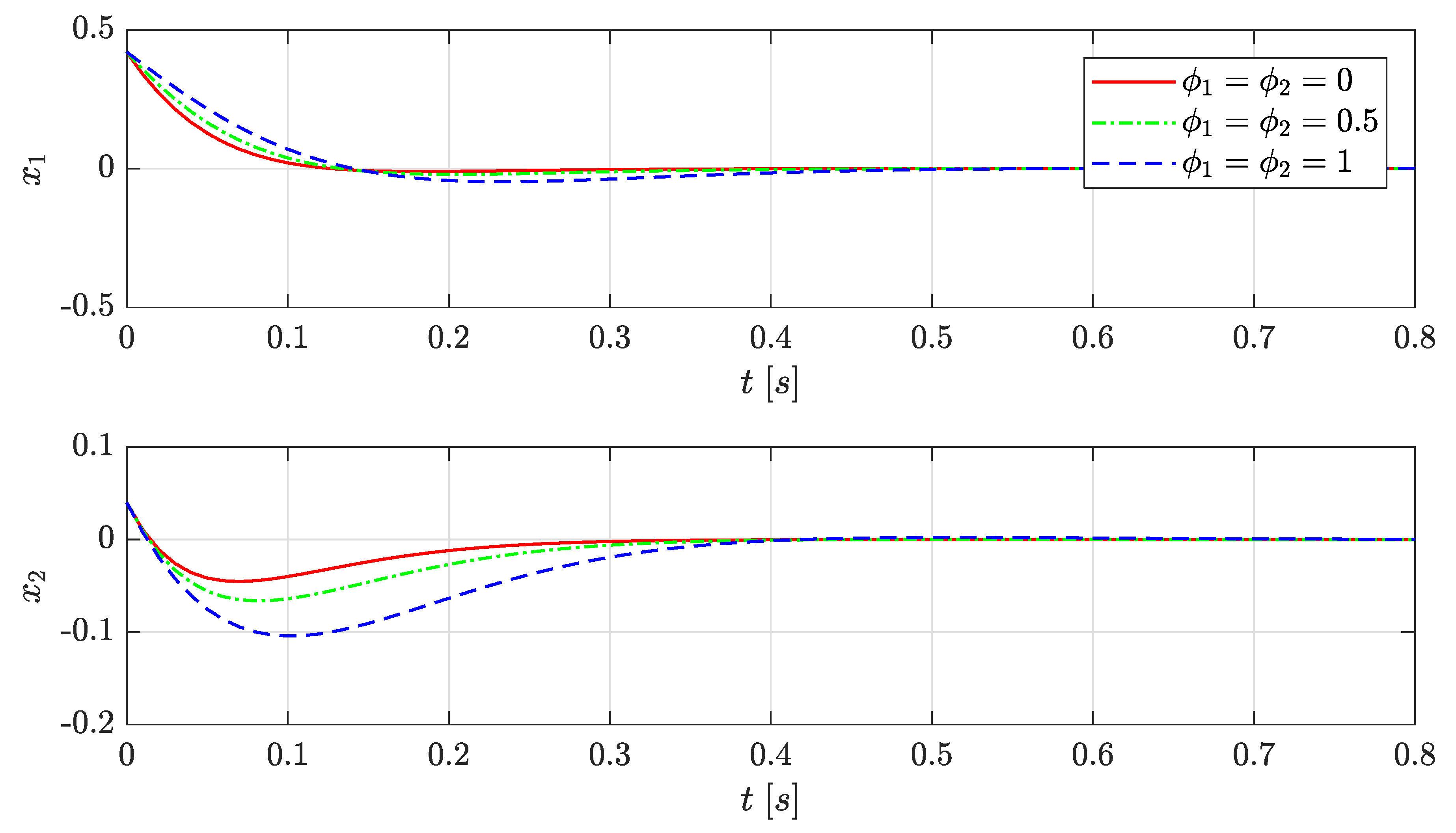
The purpose of Scenario I is to evaluate the closed-loop system stability and its closed-loop performance for a given initial condition with three different constant values of the control input saturation. To do this, we simulate the closed-loop response from an initial state $x\left(0\right)={[0.42,0.04]}^T$ and $\theta \left(t\right)=1-{\mathrm{e}}^{-t}$. Finally, fixing the frozen values of ${\varphi }_1={\varphi }_2=0$, ${\varphi }_1={\varphi }_2=0.5$ and ${\varphi }_1={\varphi }_2=1$, thus obtaining instantaneous saturation limits values ${\gamma }_1=15$ and ${\gamma }_2=7.5$, ${\gamma }_1=12.75$ and ${\gamma }_2=6.37$ and ${\gamma }_1=10$ and ${\gamma }_2=5$, respectively.

As shown in Figure 2, the closed-loop system stability is guaranteed for all the values of ${\gamma }_1$ and ${\gamma }_2$ that were mentioned. Moreover, note that the system’s response that was evaluated with the scheduling parameters ${\varphi }_1={\varphi }_2=0$, corresponds to the maximum allowed limit values of ${\gamma }_1$ and ${\gamma }_2$, obtaining the fastest system response and showing that the designed LPV state-feedback controller is able to adjust the system’s performance depending on the different values taken by $\gamma$.

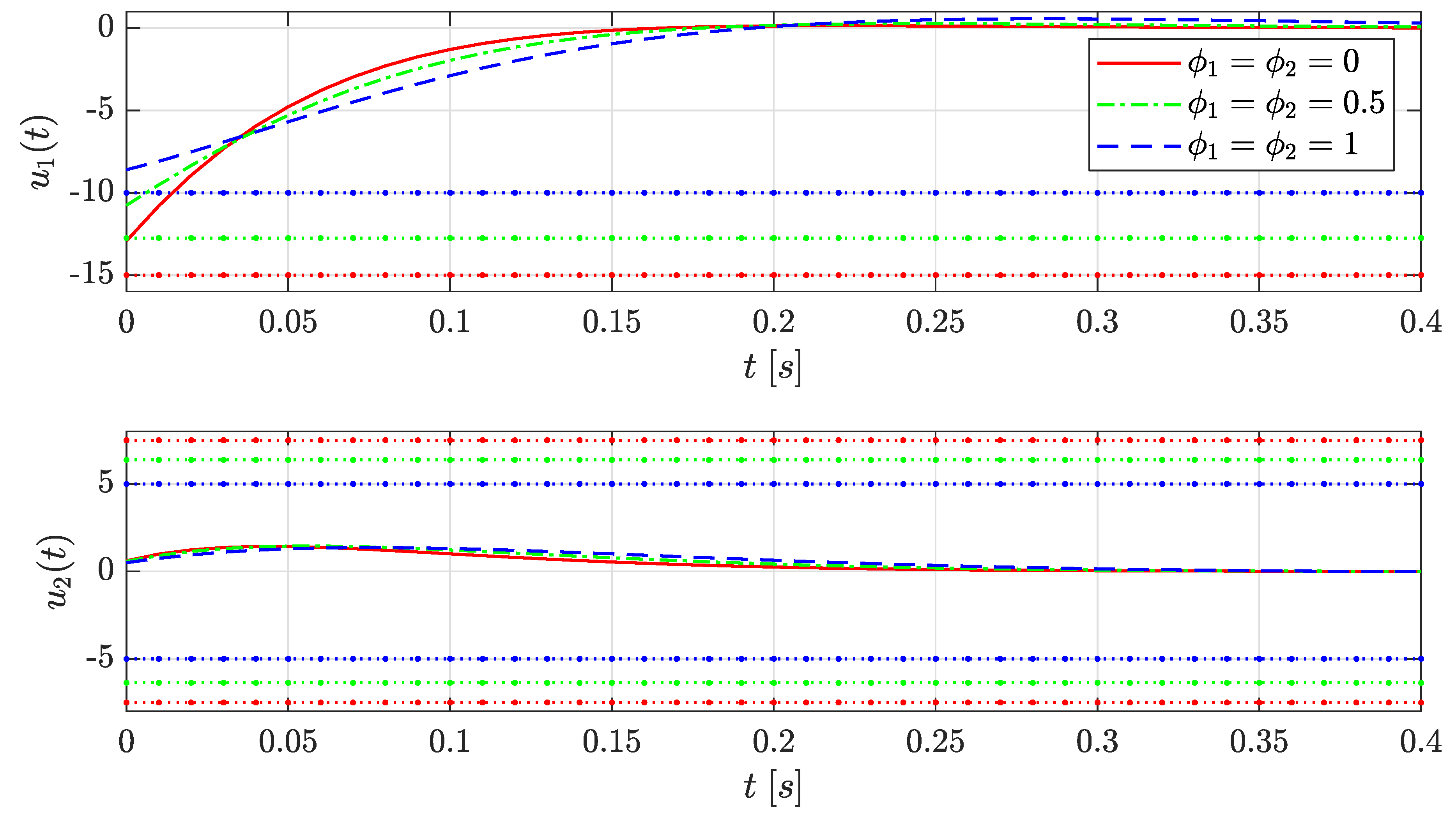
Figure 3 shows the instantaneous values of the saturation limit of $u_1$ and $u_2$ for the three frozen values of ${\varphi }_1$ and ${\varphi }_2$ and the evolution of the control signals. For illustrative purposes, since the signal $u_1$ takes only negative values during the system’s response, only the lower bound of the saturation is plotted. As a variation of the saturation limit occurs, the input signal changes as a result of the adaptability capacity of the designed controller. For example, the interval of linearity of the control signal $u_1$ corresponds to $[-15,15]$ when ${\varphi }_1={\varphi }_2=0$ and to $[-10,10]$ when ${\varphi }_1={\varphi }_2=1$. Note that if the controller gain corresponding to ${\varphi }_1={\varphi }_2=0$ had been used for the case in which ${\varphi }_1={\varphi }_2=1$, then saturation would have occurred.

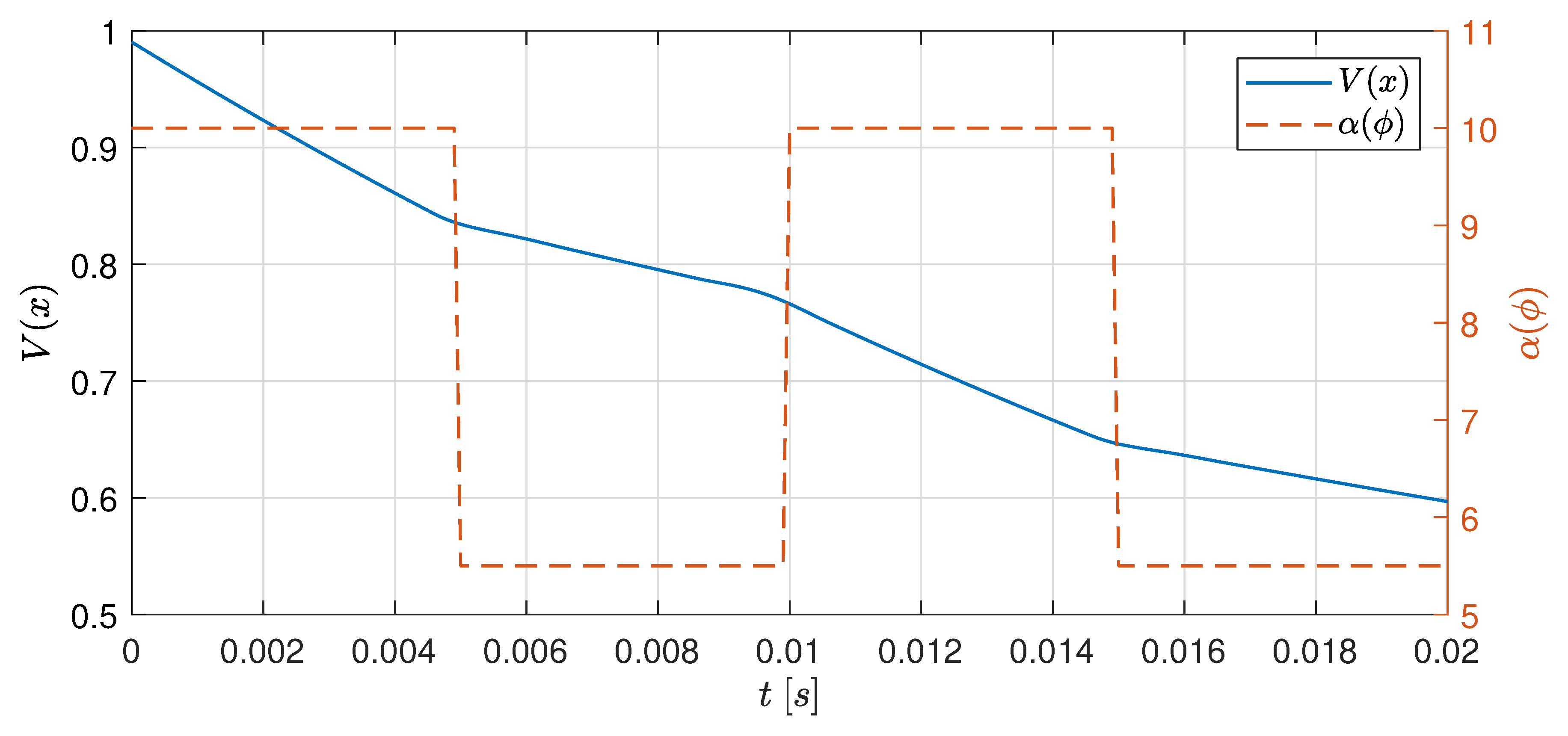
Figure 4 shows the evolution of the Lyapunov function $V\left(x\right)$ for the three frozen values of ${\varphi }_1$ and ${\varphi }_2$, which correspond to guaranteed decay rates of 10, 5.5 and 1 respectively. It can be seen that the largest decay rate corresponds to the fastest closed-loop system response, whose saturation scheduling parameters are ${\varphi }_1={\varphi }_2=0$ and $\alpha \left(\varphi \right)=10$. Also, all the functions are under the unit value, hence it is guaranteed by design that none of the control inputs saturates, as already shown in Figure 3.

5.2. Scenario II

Scenario II shows the adaptability of the designed controller to changes in $\gamma$ along the transient response of the closed-loop. We consider $x\left(0\right)={[0.42,0.04]}^T$ and $\theta \left(t\right)=1-{\mathrm{e}}^{-t}$. Also, we fix $sat\left(u_2\right)={\overline{\gamma }}_2$ and we vary $sat\left(u_1\right)$ such that it switches between its known limits ${\overline{\gamma }}_1$ and ${\underline{\gamma }}_1$.

Figure 5 shows that the designed LPV state-feedback controller is able to adapt the generated control signal $u_1$ taking into account the changes in $sat\left(u_1\right)$.

Figure 6 shows the evolution of the Lyapunov function $V\left(x\right)$, which decreases slower when the guaranteed decay rate $\alpha \left(\varphi \right)=5.5$, as a result of fixing ${\varphi }_2=0$ and faster when $\alpha \left(\varphi \right)=\overline{\alpha }$. As a consequence, the closed-loop system performance is modified online according to changes in the saturation limits.

6. Conclusions and Future Work

In this paper, the problem of designing an LPV state-feedback controller that takes into account the time-varying saturation limits has been investigated. The design procedure corresponds to checking the feasibility of an appropriate set of LMIs, which can be solved efficiently using available solvers. Finally, the results obtained in the illustrative example correspond to the case where the LPV state-feedback controller designed following the proposed methodology is evaluated in an LPV mathematical system with time-varying boundaries, showing that the controller guarantees the closed-loop stability and its capacity of adjusting the system’s performance in front of the variability of the saturation limits.

Future work will focus on applying the procedure described in this paper to design an LPV controller using robust control techniques combined with a model reference control for UAV vehicles. Moreover, in order to deal with exogenous disturbances, for example, wind gusts in the application of UAV control, the results presented in this paper will be extended to the case where disturbance rejection is considered.