An Environmental Perception Framework for Robotic Fish Formation Based on Machine Learning Methods

Abstract

Autonomous Underwater Vehicle (AUV) has become a hotspot in the field of robot in recent years. As a special kind of AUV, the robotic fish can achieve better propulsion efficiency and maneuverability than traditional AUVs. Studies show that robotic fish formation can save energy and perform more complex tasks than single robotic fish, but it is difficult to maintain a stable formation because the nearby environmental condition is hard to obtain. Inspired by the lateral line system (LLS) of fish, this paper constructs a predictive model of flow velocity and a judgement model of spacing between individual platforms for robotic fish formation through monitoring sensors on robotic fish surface. The models are built by methods of polynomial fitting and neural networks based on Computational Fluid Dynamics (CFD) simulation. The results show that the flow velocity predicted by our model could reduce the error to $0.4\%$, and the spacing judgement accuracy could reach at least 80%. The findings are useful for maintaining a stable formation and will provide significant guidance for the control of robotic fish formation and sensor installation position on the robotic fish surface.

1. Introduction

In today’s world, Autonomous Underwater Vehicles (AUVs) are implemented for a variety of tasks, including ocean surveys, mine clearance and data collection in the ocean and river environments [1]. It is a well known fact that, in nature, the fish propels itself by the coordinate motion of its body, fins, and tail, achieving higher propulsive efficiency and better maneuverability than the conventional AUVs powered by rotary propellers with the same power consumption [2]. To improve the efficiency of AUVs, more research studies are performedthe research on application, design, and control of underwater robotic fish in recent years [3,4,5,6,7,8,9].

A single robot with multiple capabilities cannot necessarily accomplish a complicated task successfully, an intended job whereas a robot swarm in which each robot has its own functions, can be more flexible, robust, and cost-effective and do complex tasks [10]. Recent studies [11,12,13,14,15] show that robotic fish formation can improve swimming efficiency. However, in the underwater environment, the velocity and viscosity of fluids, the complex geometry environment condition and even the interaction between robots can affect the stability of underwater robots formation. It is necessary for a robotic fish in a formation to get basic environmental information around itself, such as the inlet flow velocity and the spacing between itself and other robotic fish, which are useful for stable formation. With an underwater robot formation, unlike air or land robots, it is difficult to obtain the information through traditional means such as communication, GPS, and acoustic or visual systems [1,16].

Fish have a unique sensory system, lateral line system (LLS), which helps them sense fluid changes and the spacing between themselves and other objects. It has a great significance for predation, avoiding enemies, breeding and formation swimming [17,18,19,20]. In recent years, researchers try to incorporate LLS into engineering applications as an alternative method for sensing the fluid environment around AUV. Venturelli et al. [21] adopted laterally distributed parallel pressure sensor arrays and presented methods for the analysis of the surrounding steady and unsteady flows to provide a simplistic mimic of the fish’s posterior lateral line organ, which can extract control-related information. Yanagitsuru et al. [22] used pressure sensors to detect flow parameters (flow speed, vortex shedding frequency, and cylinder diameter), and the results provide insight into the sensory ecology of schools of fish and give implications for the design of autonomous underwater vehicles. Inspired by the lateral line of fish, Tang et al. [23] proposed a new kind of near-field detection system to be applied to detect impending walls, approaching obstacles and other target objects. Nawi et al. [24] could detect the moving objects located in front of the sensor by an artificial lateral line flow sensor.

Our work is inspired by the LLS of fish and we try to construct the predictive model of flow velocity and the judgement model of spacing for robotic fish formation based on the monitoring sensors attached on the robotic fish surface. To get enough monitoring data for analysis, a large number of experiments should be conducted with different physical conditions. At the same time, eigenvalues should be sorted out to improve the data quality. In traditional physics experiments, the data monitored by sensors are difficult to collect, and the errors caused by instruments and materials are inevitable. In addition, some specific conditions are difficult to achieve in real physical experiments. Therefore, we use the numerical simulation method based on Computational Fluid Dynamics (CFD) in this work.

Zhou et al. [25] used CFD methods to investigate the hydrodynamics of bio-inspired fish swimming, especially the spatial distribution and temporal variation of the near-body pressure of fish are studied. They also provided an algorithm to predict the inlet flow velocity by using the near-body pressure at distributed spatial points. Lin et al. [26] numerically studied the hydrodynamics of AUV at different speeds and analyzed the spatial distribution of the near-body pressure over the whole computational domain. Husaini et al. [27] studied the drag variation by choosing two position arrangement of cooperative AUV. Jagadeesh [28] presented a comparative assessment of the variation of drag characteristics over cooperative axisymmetric bodies at zero angle of attack. However, these original studies are all based on a single entity or the conventional AUVs formation. In robotic fish formation, the disturbance of flow caused by the swing of fish affect the data measured by sensors. It is necessary to study the perception of robotic fish formation further. Therefore, this paper studies the relationship between the pressure of fish surface and the inlet flow velocity, the spacing between individual members in simple fish formations. To be specific, the main contributions are summarized as follows:

• We construct the models of basic environment perception for different robotic fish formations. Two specific formations, tandem and phalanx, are discussed in detail. We analyze the hydrodynamic phenomena of through the flow fields, including the wake effects in the tandem formation and the pressure distribution in the phalanx formation. For the tandem formation, the robot swimming in the front will generate flow in the wake, thus the fish swimming downstream will be affected by the unsteady flow. For the phalanx configuration, the effect of the lateral flow oscillating will be considered.
• We adopt machine learning methods to generate our models using the simulation results as the sample data. Specifically, the predictive model of the flow velocity is constructed by polynomial fitting and the judgement model of spacing between robotic fish platforms is developed based on the method of neural networks. Our predictive models could reduce the error to $0.4\%$, and the spacing judgement accuracy could reach at least 80%.
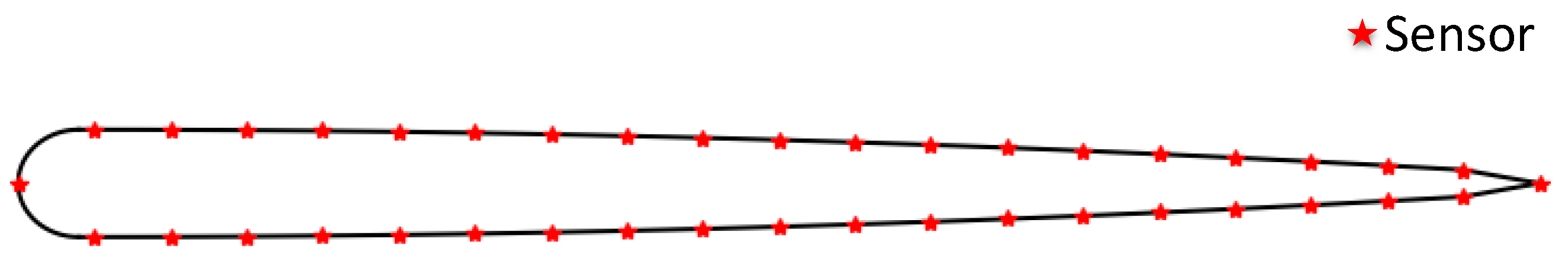
• We analyze the data monitored by sensors at different positions and find that sensors located from the head to about one-third point of the front body are more useful, while the data monitored by sensors near the tail is unstable due to the large swing amplitude at the latter part of the fish body.

[In this study, we present simulations the robotic fish usingWe outline and simulate the robotic fish based on the open-source software OpenFOAM [29,30,31], and construct the mathematical models by the methods of polynomial fitting and neural networks. The rest of the paper is organized as follows. Section 2 describes the kinematic and geometry models of robotic fish, and the CFD numerical method. Section 3 constructs the predictive model of the inlet flow velocity for single robotic fish. Section 4 constructs the predictive models of the inlet flow velocity for different formations separately. Section 5 gives the judgement models of the spacing between individual platforms for different formations separately. Conclusions are drawn in the final section.

2. Models and Methods

2.1. Kinematic Model

In nature, fish mainly adopt a wavy swing mode of propulsion. In 1926, Breder [32] proposed two models of fish swimming, one of which was the body and/or caudal fin propulsion (BCF) model, which had higher swimming speed and propulsion efficiency. In our work, we use the swimming model of anguilliform swimmers, which is one of the BCF models. The kinematic equation was specified by Carling [33] as follows:

$$y(s,t)=0.125\frac{s/L+0.03125}{1.03125}sin\left(2\pi (\frac{s}{L}-\frac{t}{T})\right),$$

(1)

where $y(s,t)$ is the lateral undulation of the midline, s is the arc length (measured from the nose) along the midline of the body, L is the body length, and T is the undulation period. Controlled by this equation, the wavelength of the body undulations is L, and the maximum lateral excursion of the tail is $0.125L$.

2.2. Geometric Model

For the above kinematic model, the three-dimensional effect of anguilliform swimmers can be neglected [25]. Therefore, we adopt the two-dimensional model in this work and only consider the robotic fish [in the same 2D planeat the same level. We use a cross-section of the three-dimensional fish body that is in the work of Kern and Koumoutsakos [34] as the geometrical model. The half outline of the two-dimensional fish body is described by $w\left(s\right)$, which is defined as analytical functions of s. The analytical description of $w\left(s\right)$ is divided into three regions:

$$w\left(s\right)=\left\{\begin{array}{cc}\sqrt{2w_{h}s-s^2}\hfill & \hfill 0\le s<s_h\\ w_h-(w_h-w_t){\left(\frac{s-s_h}{s_t-s_h}\right)}^2\hfill & \hfill s_h\le s<s_t,\\ w_t(L-s)/(L-s_t)\hfill & \hfill s_t\le s\le L\end{array}\right.$$

(2)

where $w_h=s_h=0.04L$, $w_t=0.01L$ and $s_t=0.95L$. Figure 1a shows the half outline of the straight body.

2.3. Simulation Method

2.3.1. Numerical Method

The numerical method in this work uses an arbitrary Lagrangian–Eulerian (ALE) method [35,36,37] to simulate fish moving in the fluid, which is consistent with the method in our previous work [38]. The governing equations of ALE formulation for the two-dimensional viscous incompressible flow are expressed as follows:

$$\nabla ·\mathit{u}=\mathbf{0},$$

(3)

$$\frac{\partial \mathit{u}}{\partial t}+\mathit{c}·\nabla \mathit{u}=-\frac{\nabla P}{\rho }+\nu {\nabla }^2\mathit{u}+\mathit{b},$$

(4)

where $\rho$ and $\nu$ denote the density and the kinematic viscosity of the fluid, respectively; P and $\mathit{u}$ represent the pressure and velocity of the flow, respectively; $\mathit{b}$ is the body force per unit mass; and $\mathit{c}$ is the convective velocity which represents the relative velocity between the moving mesh and the fluid. The boundary conditions are set as follows: uniform velocity at the inlet, constant static pressure and zero-gradient velocity at the outlet, slip wall at the lateral boundaries, and no-slip wall on the surface of the robotic fish. The interaction of the fish and the fluid is realized by setting a no-slip boundary condition on the robot surface and introducing a relation:

$${\mathit{u}}_b={\mathit{u}}_f,$$

(5)

where ${\mathit{u}}_b$ is the fish body velocity and ${\mathit{u}}_f$ is the fluid velocity at the surface of fish body.

The governing equations are discretized by a finite volume approach with the second-order backward scheme in time and second-order liner scheme in space. The pressure-implicit split-operator (PISO) algorithm [39] is used to solve Equations (3) and (4) for velocity and pressure. The whole computational domain is decomposed by triangle mesh, as illustrated in Figure 1b. As the fields around the undulating fish may have a large gradient, mesh near the robotic fish is refined with high resolution. In addition, we need to obtain data such as pressure on the surface of robotic fish, so the mesh of the surface should be very fine. The surface of the fish body is composed of 230–280 cells. All simulations were based on the mesh scale from $2.5\times {10}^5$ to $4.5\times {10}^5$ cells, which passed the test of grid-independence for our two-dimensional simulations. We used a parallel dynamic mesh method based on the radial basis function to move mesh on OpenFOAM [40,41].

In this study, we use the kinematic pressure, which is the ratio of pressure to the density of the fluid. In Equation (4), the kinematic pressure is equal to $\nabla P/\rho$. The kinematic pressure is considered as incompressible and its absolute value is taken relative to the outlet pressure. The outlet pressure is set to 0. The parameter $\mathit{b}$ in Equation (4) does not include gravity, thus we do not need to consider buoyancy effects. Simply, the kinematic pressure is independent of water depth. The kinematic pressure of the robotic fish surface is caused by the disturbance of the surrounding fluid. It should be noted that, in this study, only the kinematic pressure is used in simulations and it is abbreviated as p.

2.3.2. The Sampling Position

In this study, the number of sensors on the robotic fish can be increased as much as needed since the pressure sensors are virtual. We use the simulation experiments to determine the appropriate position of sensors. Limited by computational resources, time costs, experimental costs and the size of real sensors, we choose 40 sensors to complete our work. Our simulation is based on the discrete method, so we can not simulate an infinite number of sensors. Anyway, increasing the number of virtual sensors can improve accuracy, but limited by computational resources, time costs and experimental costs, we choose a total of 40 sensors to complete our work. Besides, limited by the size and cost of real sensors, the number of pressure sensors of the robotic fish surface is limited. The kinematic pressure caused by fluid disturbance is different at the different surface position. Therefore, we set a series of pressure sensors on different sampling positions on the robotic fish surface. The x coordinates of sensors are $\left\{xi\right|xi=0.05L\times i,0\le i\le 20,$ where $L$ is the length of robotic fish}. The sensor at the robotic fish head is named as $S_h(i=0)$, and sensor $S_t$ [is locatedlocates at the robotic fish tail $(i=20)$. Two pressure sensors are set symmetrically on both sides of the body at position x, which are called pair sensors. Pair sensors are coded from sensor 1 to sensor 19, defined as $S_i$, $1\le i\le 19$. $S_{iL}$is located on the left side of robotic fish body, and $S_{iR}$ is on the right side. The sensor positions are shown in Figure 2. In this work, all sensors are pressure sensors and we calculate the kinematic pressure by the mean values in a swimming cycle. The kinematic pressures on pair sensors are recorded as $p_{iR}$ and $p_{iL}$ $(1\le i\le 19)$. As for the head and tail, the kinematic pressure are recorded as $p_h$ and $p_t$.

2.3.3. The Grid Independence

The size of the computational domain is $25L\times 8L$ (L is the length of the robotic fish body), and the robotic fish swims in the middle of the whole computational domain. Because we need to consider the pressure data of a specific position on the surface of the robotic fish in our work, we need a fine body-fitted grid to ensure the accuracy of the pressure. We build the coarse and fine unstructured grids that produce $M1$ (141,778 cells), $M2$ (26,2304 cells) and $M3$ (314,832 cells), respectively, where the size of a cell on the robotic fish surface is much smaller than the spacing between sensors. The grid-independence analysis is performed by comparing the pressure at the same position ($p_{2R}$) on the surface of the single robotic fish obtained with the three meshes. As shown in Figure 3, the pressure obtained with $M2$ and $M3$ are almost identical and the maximum relative difference is less than $1\%$. The same mesh scale as $M2$ is adopted in the following simulations.

3. The Velocity Prediction of Single Robotic Fish

In this section, we discuss the relationship between the kinematic pressure of the robotic fish surface and the velocity U of inlet flow. The kinematic pressure of the robotic fish surface is caused by the disturbance of the surrounding fluid. The disturbance of fluid is influenced by both the inlet flow velocity and the swing of the robotic fish. In this work, the fish swims with certain wave motion parameters and the inlet flow velocity is the most important factor affecting the kinematic pressure of single fish.

3.1. The Simulated Experiment Settings

The flow field is stable and the inlet velocity is U. We set the Reynolds number $Re$from hundreds to thousands. In general, the factors affecting the kinematic pressure include time, sampling position, relative velocity and swimming parameters of robotic fish. In this work, the swimming parameters are stable. We consider the periodic variation of kinematic pressure and the sampling position.

By 2017, the fastest swimming robotic fish was made by Li Tiefeng et al. [42]. Its body length was about 9.3 cm, and its maximum swimming speed was 13.5 cm/s, about $1.5$ times the length per second. Combining the current research status of robotic fish, we set the inlet velocity U from $0L/s$ to $2.5L/s$ (L is the length of robotic fish). The velocity settings for training predictive models are shown in

Table 1. The velocity setting for training.

U (L/s)
0, 0.2, 0.4, 0.6, 0.8, 1.0, 1.2, 1.4, 1.6, 1.8, 2.0, 2.5

.

3.2. The Results Analysis

The single robotic fish is not disturbed by factors other than water flow. The data monitored by symmetrical sensors on both sides of the fish body are symmetrical in a cycle of fish swimming, as shown in Figure 4. It is helpful to calculate the sum of two sensors at the same x coordinate in a swimming period, which leads to stable and reliable results. Therefore, in this section, $p_0=p_h$, $p_{20}=p_t$, and $p_i=p_{iR}+p_{iL}$, ($1\le i\le 19$). We plot the change of $p_i$ with the inlet flow velocity U and select several positions with obvious change for further study. As shown in Figure 5, the kinematic pressure of the head ($p_0$) and $p_1$ to $p_7$ of the single fish varies dramatically and monotonously, and these data can be used as training data for predicting inlet flow velocity. The relationships between other $p_i(8\le i\le 16)$ and U are almost the same as that between $p_7$ and U. However, due to the swimming characteristics of the robotic fish, the tail has large amplitude, and the kinematic pressures ($p_{17}$–$p_{20}$) monitored by sensors near the tail are unstable, which are not suitable for prediction.

3.3. The Construction and Validation of Predictive Models

We used polynomial regression to predict the inlet flow velocity. The construction phase of predictive models and their validation were done by a powerful library called $scikit$-$learn$, which is a Python module that integrates many machine learning algorithms [43]. Our predictive models are presented as a polynomial in the following form:

$$U=C_0+C_1\times p_i+C_2\times p_i^2+C_3\times p_i^3+\cdots +C_n\times p_i^n,$$

(6)

where $C_j(0\le j\le n)$ is the coefficient of the polynomial, n is the order of the polynomial, and $p_i(0\le i\le 7)$ has limited scope to ensure the validity of polynomial.

We used the corresponding relations of $p_i(0\le i\le 7)$ and U to train predictive models, respectively, and set a series of U to validate predictive models. The velocity settings for validating predictive models are shown in

Table 2. The velocity setting for validating.

U ($\mathit{L}/\mathit{s}$)
0.1, 0.3, 0.5, 0.7, 0.9, 1.1, 1.3, 1.5, 1.7, 1.9, 2.1, 2.2, 2.3, 2.4

. While building the predictive model, we used different orders and calculated the training error. Then, we used the test data to validate the predictive model and calculate the predictive error. Errors are the mean square deviation of standard and calculated values. The training and predictive error of these models are shown in

Table 3. The training and predictive error.

	${\mathit{p}}_0$			${\mathit{p}}_1$
order (n)	training error	predictive error	order (n)	training error	predictive error
1	0.04600	0.02912	1	0.03043	0.02046
2	0.01186	0.00821	2	0.00955	0.00586
3	0.00407	0.00487	3	0.00360	0.00323
4	0.00205	0.00482	4	0.00159	0.00300
5	0.00121	0.01619	5	0.00079	0.00586
6	0.00061	0.14485	6	0.00043	0.02093
	${\mathit{p}}_2$			${\mathit{p}}_3$
order (n)	training error	predictive error	order (n)	training error	predictive error
1	0.03402	0.02268	1	0.02649	0.01781
2	0.00853	0.00550	2	0.00677	0.00410
3	0.00295	0.00291	3	0.00246	0.00210
4	0.00125	0.00305	4	0.00104	0.00218
5	0.00059	0.00684	5	0.00045	0.00408
6	0.00030	0.02744	6	0.00022	0.01208
	${\mathit{p}}_4$			${\mathit{p}}_5$
order (n)	training error	predictive error	order (n)	training error	predictive error
1	0.02630	0.01775	1	0.02528	0.01667
2	0.00621	0.00378	2	0.00521	0.00310
3	0.00219	0.00184	3	0.00195	0.00159
4	0.00093	0.00199	4	0.00084	0.00191
5	0.00040	0.00380	5	0.00035	0.00374
6	0.00019	0.01089	6	0.00017	0.01018
	${\mathit{p}}_6$			${\mathit{p}}_7$
order (n)	training error	predictive error	order (n)	training error	predictive error
1	0.02425	0.01553	1	0.02203	0.01384
2	0.00434	0.00249	2	0.00367	0.00203
3	0.00178	0.00139	3	0.00162	0.00123
4	0.00079	0.00193	4	0.00068	0.00181
5	0.00032	0.00372	5	0.00026	0.00300
6	0.00016	0.00974	6	0.00013	0.006952

, respectively.

We can find that the training error is smaller when the order of the polynomial is higher, but the predictive error does not always become smaller. The problem is called overfitting: If we set the order of the polynomial into our model creation too high, the model will be created perfectly, but only for the training data. Therefore, we think the best model can obtain the minimum predictive error and we use red to mark it in Table 3. Then, we plot the training data, predictive data and the predictive model in Figure 6. We can see how well the predictive model fits the data. However, the predictive models trained by $p_0$ and $p_1$ are not monotonic in the limited scope and the fourth-order polynomials are overfitted. We select the third-order polynomials trained by $p_0$ and $p_1$, respectively, and the fitting images are shown in Figure 7.

Through Figure 6 and Figure 7 and Table 3, we can get the best predictive model with the minimum predictive error in all polynomials, that is, the polynomial predicted by $p_7$ (the kinematic pressure of sensor $S_7$ at $x=0.35L$) is as follows:

$$U=0.0006+(-5.9127)\times p_7+(-6.3910)\times p_7^2+(-3.3478)\times p_7^3-1\le p_7\le 0,$$

(7)

Equation (7) is applicable to the velocity prediction of single robotic fish. In the case of two or more fishes, the fish is affected by the swing of other adjacent fish, the kinematic pressure of which is different from that of single robotic fish.

4. The Velocity Prediction of Two Robotic Fishes

In this section, we discuss the case of two robotic fishes and predict the inlet flow velocity by the kinematic pressure of every robotic fish surface.

4.1. The Simulated Experiment Settings

We set the same environmental parameters as Section 3 and two formations in Figure 8 configured by two robotic fishes. For the tandem shape in Figure 8a, fishes are swimming in a line with interval spacing $dx$. In this configuration, the robot swimming in the front will generate flow in the wake, and thus the fish swimming downstream will be affected by the unsteady flow. For the phalanx configuration in Figure 8b, fishes are placed in a column with spacing $dy$, and the effect of the lateral flow oscillating is considered. For all formation configurations, fishes are swimming in the same phase difference. In each task of formation, the shape of formation (tandem or phalanx) and the appropriate spacing $\Delta d$ between robotic fishes are set in advance. The number of each fish in the formation is also given in Figure 8, the kinematic pressure of the No. 1 fish is recorded as $p{1}_i$ and the kinematic pressure of the No. 2 fish is recorded as $p{2}_i(0\le i\le 20$). We study the kinematic pressure of the robotic fish surface with the spacing $dx$, $dy$ and the inlet flow velocity U varying in

Table 4. The spacing and velocity setting.

Spacing (L)	U ($\mathit{L}/\mathit{s}$)
0.2, 0.4, 0.6, 0.8, 1.0	0, 0.2, 0.4, 0.6, 0.8, 1.0

.

The tandem formation and phalanx formation have different phenomena, thus we study the flow fields and the kinematic pressures of the tandem formation and phalanx formation separately. Then, we train the predictive models of inlet flow velocity of the two formations separately.

4.2. The Tandem Formation

In the tandem formation, two fishes can know whether they are in the front (No. 1) or at the back (No. 2). However, they cannot communicate with each other. We need to construct the predictive model of inlet flow velocity for each fish.

4.2.1. The Results Analysis

Through analyzing the flow fields of two fishes in the tandem formation shown in Figure 9, we found that the fish at the back (No. 2) is affected by the flow in the wake generated by the front fish (No. 1). When the inlet flow velocity is small, as shown in Figure 9a,c, the fluid disturbance in the vertical direction of the fish body caused by the fish body swing is large. When the spacing between the two fishes changes as shown in Figure 9a–d, the fish in the front (No. 1) is almost unaffected, but the fish at the back (No. 2) is affected differently.

For a single robotic fish, the relationships between $p_i(8\le i\le 16$) and U are almost the same as those between $p_7$ and U. However, due to the swimming characteristics of the robotic fish, the tail has large amplitude, and the kinematic pressures ($p_{17}$–$p_{20}$) monitored by sensors near the tail are unstable, which are not suitable for prediction. Therefore, we chose the data monitored by sensors $S_0$–$S_7$ and sensors near them. We calculated the mean square deviation of kinematic pressure at different spacing at a certain U, as shown in

Table 5. The mean square deviation of $p_i$ at different spacing at a certain U.

			U ($\mathit{L}/\mathit{s}$)
	0	0.2	0.4	0.6	0.8	1.0
$p{1}_0$	3.66 × 10${}^{-7}$	0.000001	0.000007	0.000021	0.000045	0.000093
$p{1}_1$	0.000139	0.000113	0.000095	0.000095	0.000142	0.000259
$p{1}_2$	0.000346	0.000197	0.000078	0.000014	0.000131	0.000500
$p{1}_7$	0.000038	0.000024	0.000015	0.000011	0.000017	0.000047
$p{2}_0$	0.002748	0.001678	0.000612	0.000316	0.000282	0.000935
$p{2}_6$	0.000249	0.000082	0.000011	0.000050	0.000087	0.000190
$p{2}_7$	0.000119	0.000022	0.000011	0.000043	0.000028	0.000034
$p{2}_8$	0.000085	0.000091	0.000017	0.000048	0.000029	0.000038

. Through analyzing the data monitored by sensors, we found that the kinematic pressures at the head of front fish (No. 1) are almost unaffected by spacing, as shown in Figure 10a and Table 5. Thus, $p{1}_0$ can be used to train the predictive model of inlet flow velocity for No. 1 fish. For No. 2 fish, the data monitored by sensor $S_7$ are less affected by spacing, as shown in Figure 10g and Table 5. We can use $p{2}_7$ $(p{2}_7=p{2}_{7R}+p{2}_{7L})$ to construct the predictive model of inlet flow velocity for No. 2 fish.

4.2.2. The Construction and Validation of Predictive Models

We used the data simulated by settings in Table 4 to train the predictive model and use the data simulated by settings in

Table 6. The spacing and velocity setting for validating.

Spacing (L)	U ($\mathit{L}/\mathit{s}$)
0.2, 0.4, 0.6, 0.8, 1.0	0.1, 0.3, 0.5, 0.7, 0.9

to validate the model. The kinematic pressures used to train and validate the predictive model are the average values of $p_i$ at different spacing at a certain U.

In Section 3, we construct the predictive model of the inlet flow velocity for single robotic fish. We compared the kinematic pressure of the No. 1 fish head ($p{1}_0$) and that of the single fish head ($p_0$) firstly at the different inlet flow velocity U. As shown on the left of Figure 11, $p{1}_0$ and $p_0$ have few differences and the predictive model of $p_0$ in Section 3 can be used to predictive U for No. 1 fish in the tandem formation. The polynomial as the predictive model for No. 1 fish is as follows:

$$U=0.1693+1.9999*p{1}_0+(-0.8366)*p{1}_0^2+0.1400*p{1}_0^3-0.1\le p{1}_0\le 0.6,$$

(8)

Then, we compared the kinematic pressure of the No. 2 fish ($p{2}_7$) and that of single fish ($p_7$) at the different inlet flow velocity U. As shown on the right of Figure 11, $p{2}_7$ and $p_7$ have some differences and the predictive model of $p_7$ in Section 3 cannot be used to predict U for No. 2 fish in tandem formation. Therefore, we construct a new predictive model for No. 2 fish and the method is the same as Section 3. While building the predictive model, we used different order of polynomial and calculated the training error. Then, we used the test data to validate the predictive model and calculate the predictive error. The training and predictive error of the model are shown in

Table 7. The training and predictive error.

$\mathit{p}{2}_7$
order (n)	training error	predictive error
1	0.00171	0.00128
2	0.00004	0.00034
3	0.00003	0.00035
4	0.00001	0.00045

.

We found that the training error and predictive error are very small when the order of polynomial $n=2$ and $n=3$. We plot the training data, predictive data and the predictive model in Figure 12, which shows that the fitting effect is almost identical when the order of polynomial is $n=2$ and $n=3$. Because the best polynomial of a single robotic fish is third-order, finally we chose the third-order polynomial as the predictive model, which is in the following:

$$U=-0.1369+(-7.3297)\times p{2}_7+(-5.4535)\times p{2}_7^2+17.1535\times p{2}_7^3-0.3\le p{2}_7\le 0,$$

(9)

Equation (9) is applicable to the velocity prediction of No. 2 fish in the tandem formation. It is worth noting that the fluid disturbance in the vertical direction of the fish body caused by the fish body swing is large when the inlet flow velocity is small. Thus, the velocity prediction less than $0.2L/s$ may not be accurate enough.

4.3. The Phalanx Formation

In the phalanx formation, two fishes can know whether they are on the left (No. 1) or on the right (No. 2). However, they cannot communicate with each other. We need to construct the predictive model of inlet flow velocity for each fish.

4.3.1. The Results Analysis

Through analyzing the contours in pressure fields of two fishes in the phalanx formation shown in Figure 13, we found that the pressure generated by the swing of fish body will affect the adjacent fish and the flow field on both sides of the fish body are not symmetrical. When the inlet flow velocity is small, as shown in Figure 13a,c, the pressure of the body surface caused by the swing of the fish is positive or negative. When the inlet flow velocity is large, as shown in Figure 13b,d, the flow has a greater impact than the swing of fish on the pressure of the body surface, which is almost negative and the pressure at the head is obvious. When the spacing between the two fishes changes, as shown in Figure 13a–d, the pressures on the adjacent side $(p{1}_{iR}$ and $p{2}_{iL})$ are affected differently by the swing of another fish.

We chooe the data monitored by sensors $S_0$, $S{1}_{iL}$ and $S{2}_{iR}(1\le i\le 7)$, ), which are located outside the phalanx formation. We calculated the mean square deviation of kinematic pressure at different spacing at a certain U, as shown in

Table 8. The mean square deviation of $p_i$ at different spacing at a certain U.

U (L/s)
	0	0.2	0.4	0.6	0.8	1.0
$p{1}_0$	0.000005	0.000021	0.000012	0.000041	0.000091	0.000249
$p{1}_{1L}$	0.000113	0.000139	0.000277	0.000469	0.000862	0.001587
$p{1}_{7L}$	0.000031	0.000032	0.000015	0.000016	0.000105	0.000275
$p{2}_0$	0.000006	0.000020	0.000033	0.000100	0.000089	0.000231
$p{2}_{1R}$	0.000021	0.000019	0.000040	0.000442	0.001458	0.003232
$p{2}_{7R}$	0.000099	0.000072	0.000035	0.000043	0.000312	0.000385

. Through analyzing the data monitored by sensors, we found that the kinematic pressures at head are almost unaffected by spacing, as shown in Figure 14a,b and Table 8. Thus, $p{1}_0$ can be used to train the predictive model of inlet flow velocity for No. 1 fish and $p{2}_0$ can be used to train the predictive model of inlet flow velocity for No. 2 fish.

4.3.2. The Construction and Validation of Predictive Models

We used the data simulated by settings in Table 4 to train the predictive model and used the data simulated by settings in Table 6 to validate the model. The kinematic pressures used to train and validate the predictive model are the average values of $p_0$ at different spacing at a certain U. In Section 3, we construct the predictive model of the inlet flow velocity for single robotic fish. We compared the kinematic pressure of the No. 1 fish head ($p{1}_0$), the kinematic pressure of the No. 2 fish head ($p{2}_0$) and that of the single fish head ($p_0$) at the different inlet flow velocity U. As shown in Figure 15, $p{1}_0$, $p{2}_0$ and $p_0$ have few differences and the predictive model of $p_0$ in Section 3 can be used to predict U for each fish in the phalanx formation. The polynomial as the predictive model for each fish in the phalanx formation is as follows:

$$U=0.1693+1.9999\times p{i}_0+(-0.8366)\times p{i}_0^2+0.1400\times p{i}_0^3-0.1\le p{i}_0\le 0.6,i=1or2,$$

(10)

For the case of two robotic fishes, No. 1 fish in the tandem formation and each fish in the phalanx formation have the same predictive models. No. 2 fish in the tandem formation has a specific predictive model.

5. The Spacing Judgement of Two Robotic Fishes

In this section, we judge the spacing between two robotic fishes by the kinematic pressures of the fish surface. Our purpose is to determine the relationship between the current spacing and the presetting spacing $\Delta d$. We only need to know whether the current spacing is greater or less than the presetting spacing $\Delta d$, but we do not need to know the exact value of the current spacing. Therefore, we choose neural networks to binary classification and construct the judgement model. 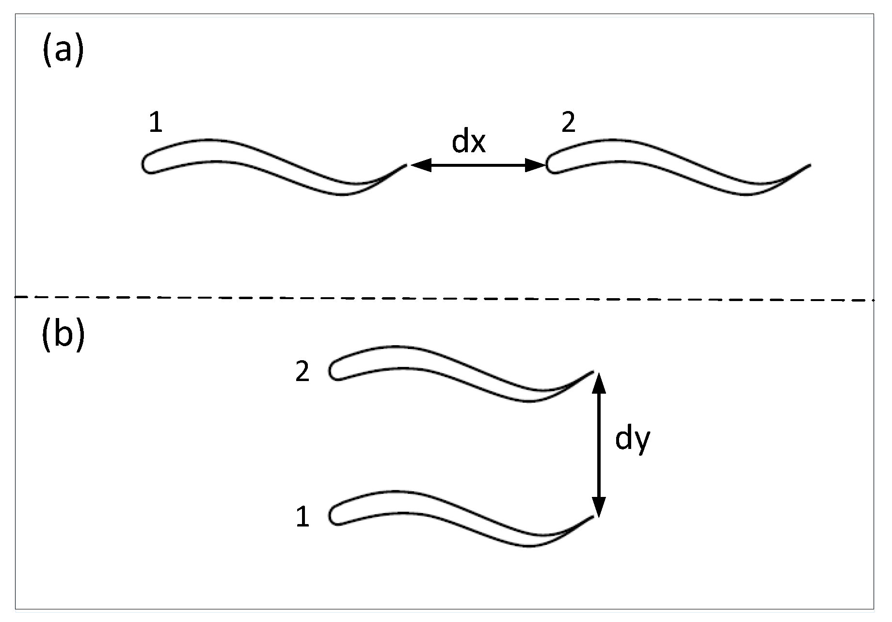The simulated experiment settings are the same as Section 4. The tandem formation and phalanx formation have different phenomena, thus we discuss the tandem formation and phalanx formation separately.

5.1. The Tandem Formation

In the tandem formation, the fish in the front (No. 1) does not need to consider the spacing between two fishes. To avoid collision and maintain the appropriate spacing $\Delta d$ in the formation, the fish at the back (No. 2) needs to judge the spacing between the two fishes. Thus, we are concerned about the kinematic pressures on No. 2 fish surface and judge the relationship between the current spacing $dx$ and the presetting appropriate spacing $\Delta d$ by the kinematic pressure on No. 2 fish surface.

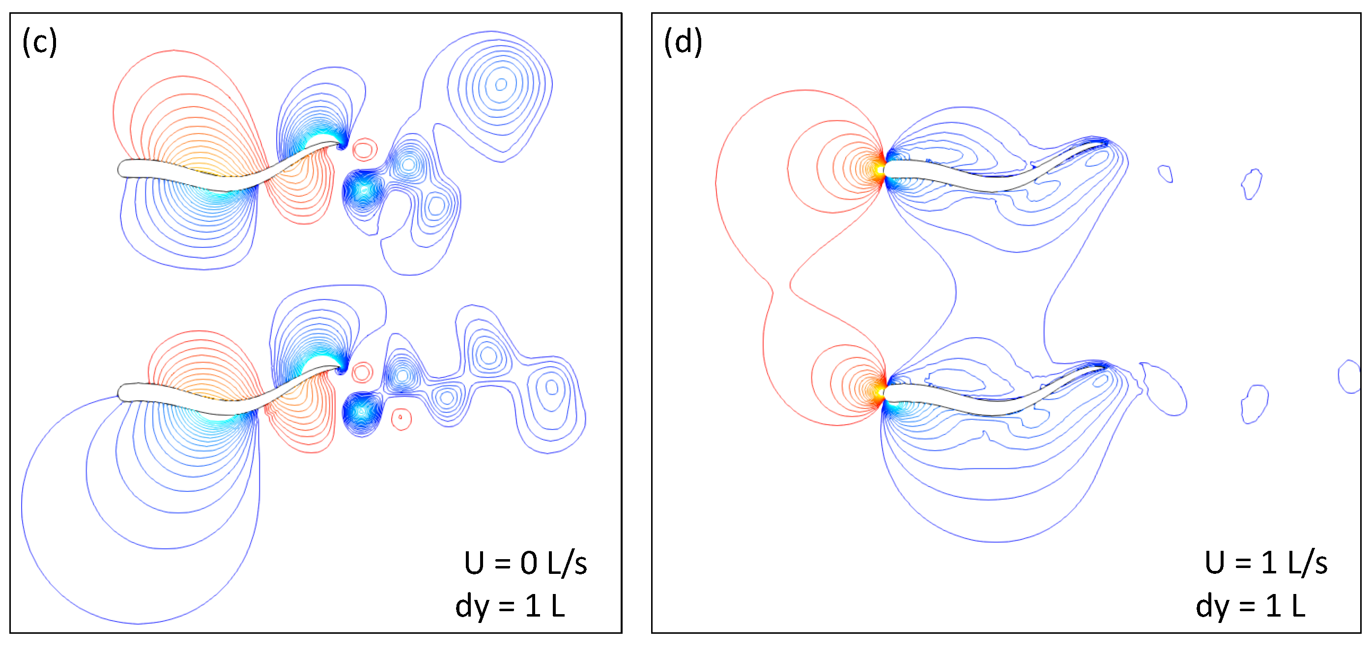
5.1.1. The Results Analysis

As presented in Section 4, we found that, for No. 2 fish in the tandem, the data monitored by sensor $S_7$ are less affected by spacing and we used $p{2}_7$ to construct the predictive model of inlet flow velocity for No. 2 fish. Since the wake of No. 1 fish mainly affects the head of No. 2 fish and its surroundings, the data monitored by sensors after $S_7$ are almost unaffected by spacing. The head of No. 2 fish is directly impacted by the wake. The data monitored by the sensor here ($S_0$) are noisy and inaccurate, as shown on the left of Figure 16. We chose the data monitored by sensors $S_3$ to judge the spacing. This position can be affected by the wake, and, because of the swing of No. 2 fish itself, the impact of the wake is not as severe as that of the head and the data monitored by these sensors $\left(p{2}_3\right)$ are stable, as shown on the right of Figure 16, which are suitable for judging the spacing.

5.1.2. The Construction and Validation of Judgement Models

Through the results on right side of Figure 16, we found that, at the different inlet flow velocity U, the relationship between $p{2}_3$ and the spacing $dx$ is different. Thus, we also need to use the kinematic pressure $p{2}_7$, which is insensitive to the spacing as a feature for eliminating the effect of inlet flow velocity. In this work, for the presetting appropriate spacing $\Delta d$, we divide the data into two categories: the label is equal to 0 when the current spacing $dx$ is less than $\Delta d$, and the label is equal to 1 when the current spacing $dx$ is greater than $\Delta d$. We construct a binary classification model by using the method of neural networks [44,45]. The model can be used to judge the relationship between the current spacing $dx$ and the presetting appropriate spacing $\Delta d$. It has one input layer, two hidden layers and one output layer, as shown in Figure 17. The input layer contains two features, $p{2}_3$ and $p{2}_7$. Each hidden layer has 128 neurons and the activation function is Rectified Linear Unit (ReLU). The output layer is the result of classification, which is equal to 0 or 1 and the activation function is Sigmoid. The loss function of the model is binary_crossentropy, and the optimizer is Adam. We used the data simulated by settings in Table 4 to train the classification model, and used the data simulated by settings in Table 6 to validate the model. We used several $\Delta d$ to construct the judgement models, and the effects are shown in

Table 9. The accuracy rate of the judgement models.

$\Delta \mathit{d}$	Accuracy Rate
0.3 L	$80\%$
0.5 L	$84\%$
0.7 L	$80\%$
0.9 L	$84\%$

.

Through the above neural network structure, we can train a judgement model to compare the current spacing $dx$ with any $\Delta d$ in a certain range.

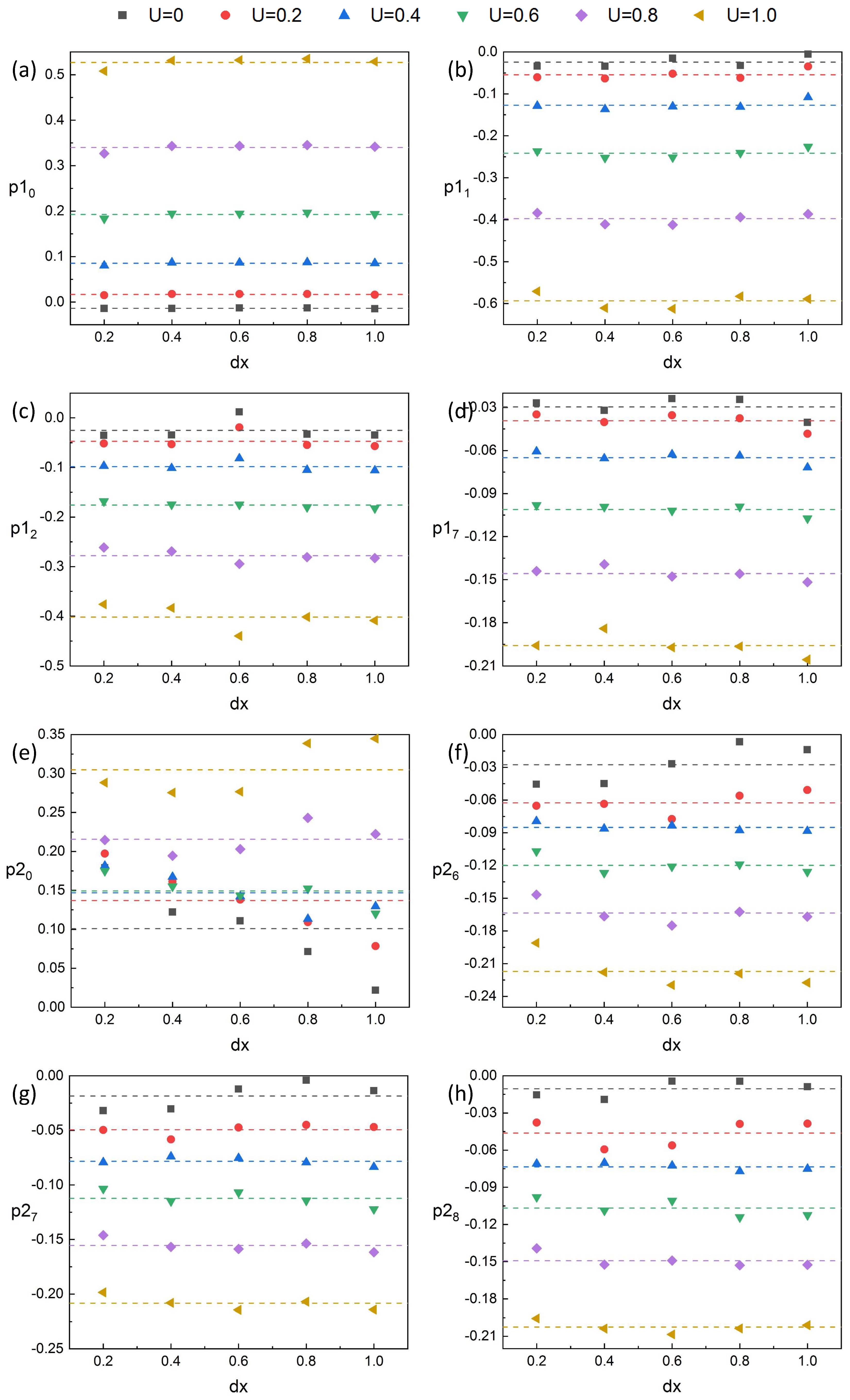
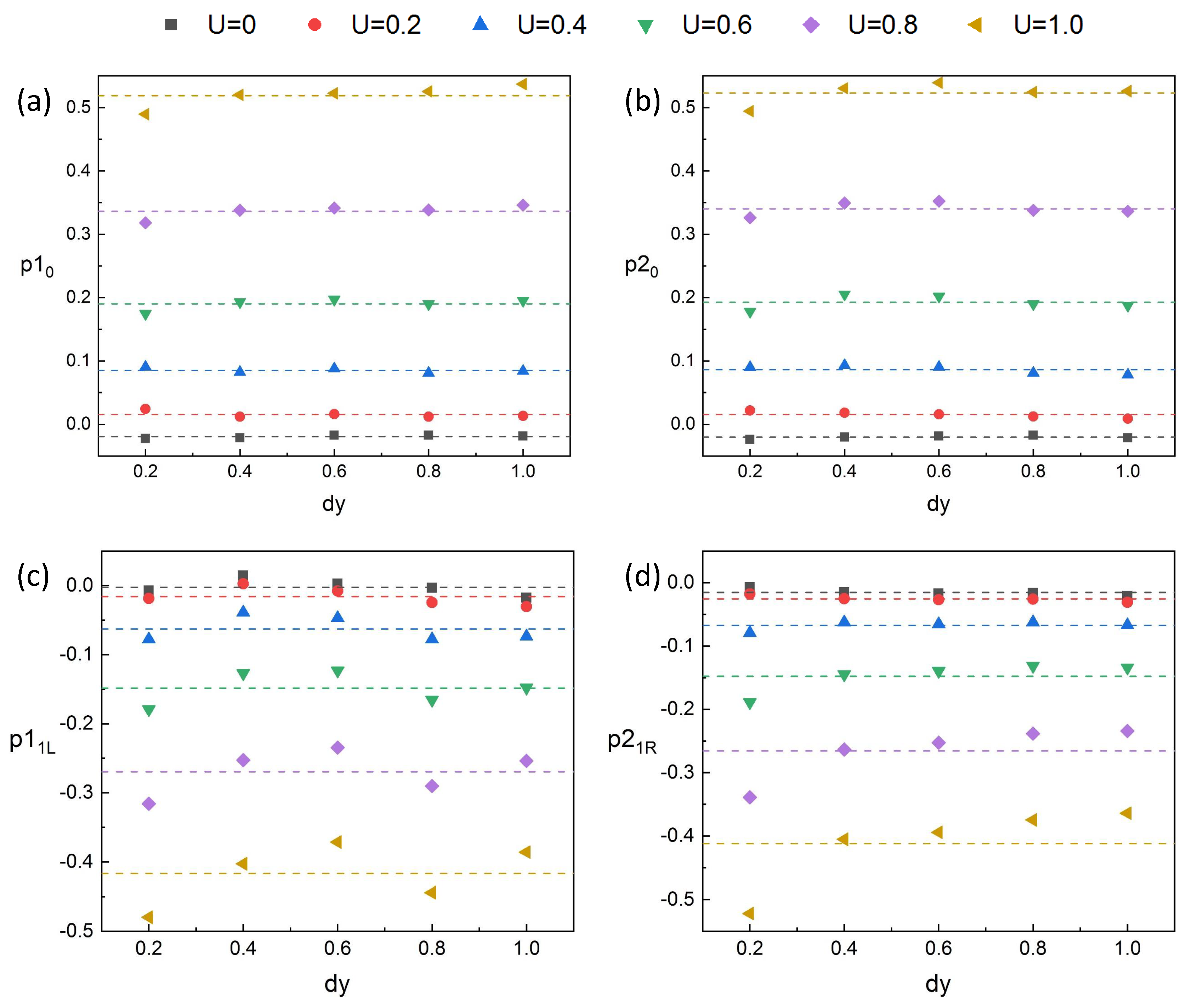
5.2. The Phalanx Formation

In the phalanx formation, to avoid collision and maintain the appropriate spacing $\Delta d$ in the formation, the fish, whether on the left (No. 1) or on the right (No. 2), needs to know the spacing between the two fishes. We are concerned about the kinematic pressure on each fish surface and judge the relationship between the current spacing $dy$ and the presetting appropriate spacing $\Delta d$ by the kinematic pressure on each fish surface.

5.2.1. The Results Analysis

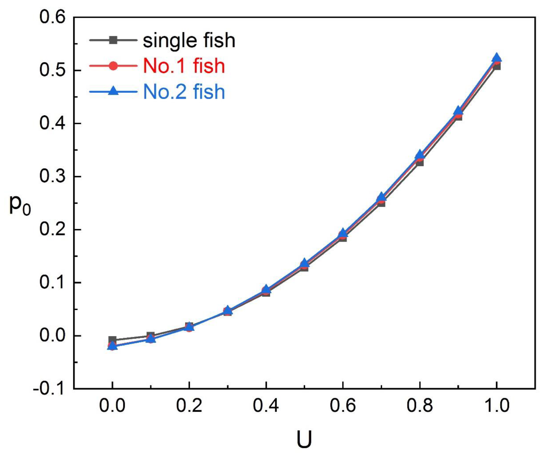
Through the results in Figure 13 (Section 4), we found that the pressure fields on the adjacent side of the two fishes overlap greatly at a close spacing in the phalanx formation. $p{1}_{iR}$ and $p{2}_{iL}$ are more susceptible to spacing than pressures on the other side ($p{1}_{iL}$ and $p{2}_{iR}$). Therefore, we calculated the kinematic pressures of the specific side of fish, which are $p{1}_{iR}$ and $p{2}_{iL}$. 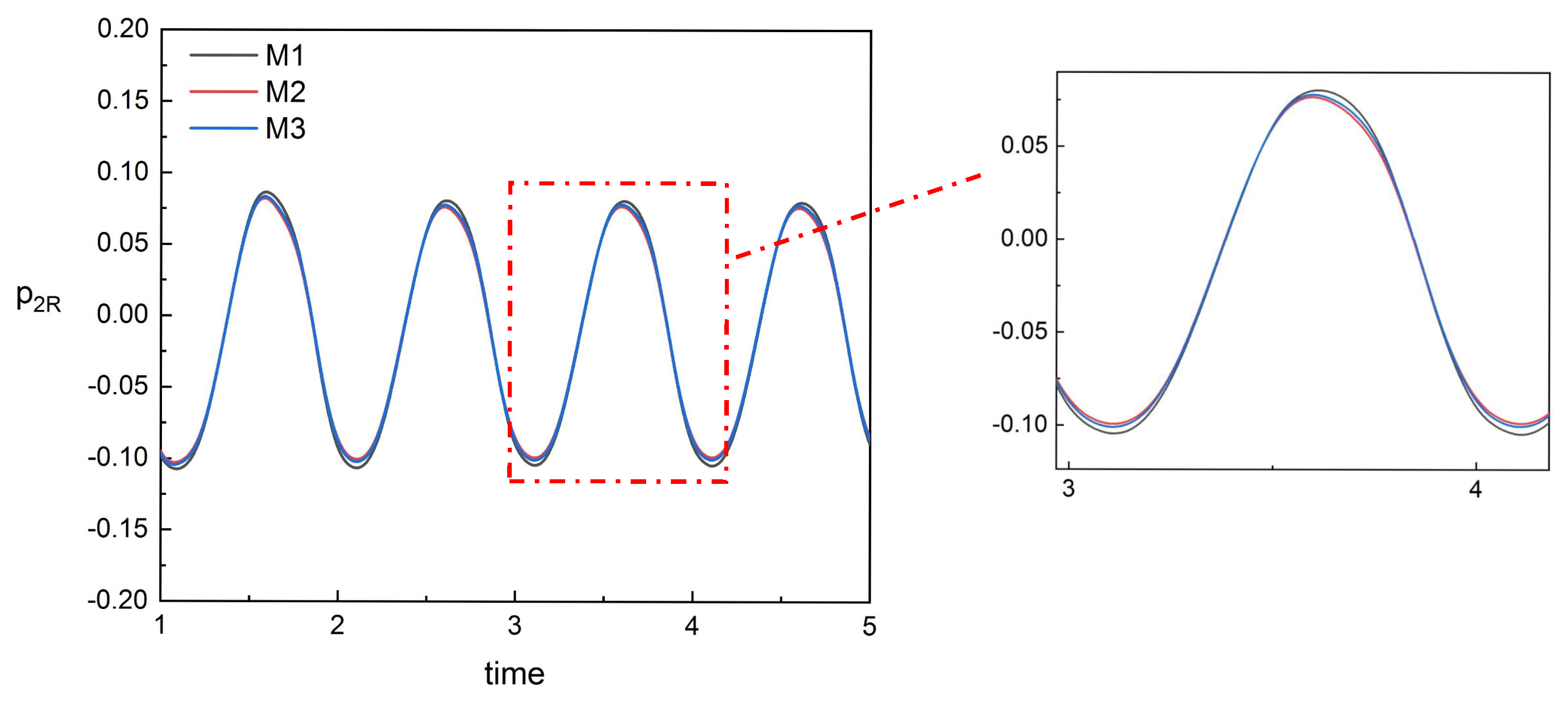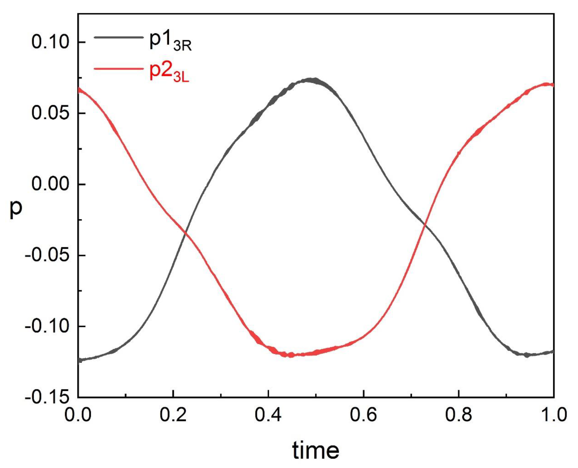We found that $p{1}_{iR}$ and $p{2}_{iL}$ are symmetrical in a cycle of fish swimming, as shown in Figure 18. The data in Figure 18 are monitored at a suitable spacing ($dy=0.4L$), which can ensure the representativeness of the rules of data at different spacing. When the inlet flow velocity is 0, the interaction of fish body swing is large, thus the rules of the data are representative at different U. Although there are some slight jitters in the data, $p{1}_{iR}$ and $p{2}_{iL}$ are approximately equal and we calculated the average of $p{1}_{iR}$ and $p{2}_{iL}$ as $p_i^{\prime }$.

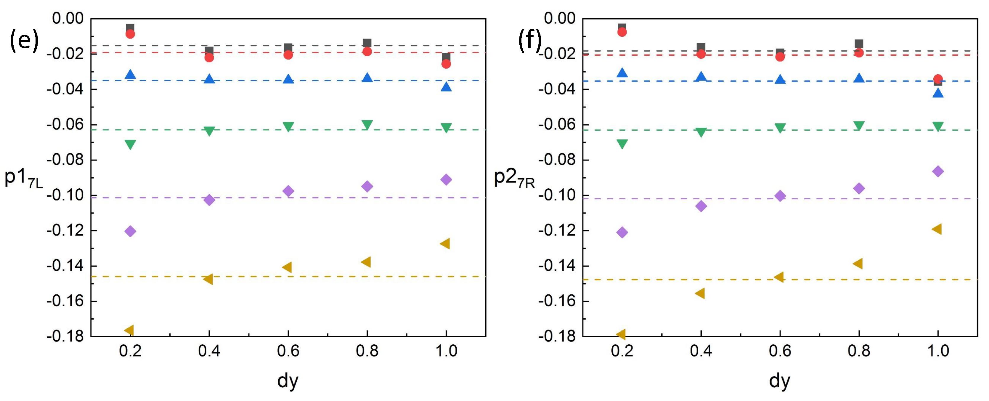
In this work, the data we mainly used are monitored by sensors $S_0$, $S_3$ and $S_7$. To save the cost of sensors placement, we give priority to the data at these positions. We used the data ($p{1}_0$ and $p{2}_0$) monitored by $S_0$, which are almost unaffected by spacing to predictive the inlet flow velocity for the phalanx formation. Thus, we consider the data monitored by $S_3$ and $S_7$ in this part. In the phalanx formation, we calculated $p_3^{\prime }$ and $p_7^{\prime }$ to discuss the relationship between the kinematic pressure and the spacing $dy$. 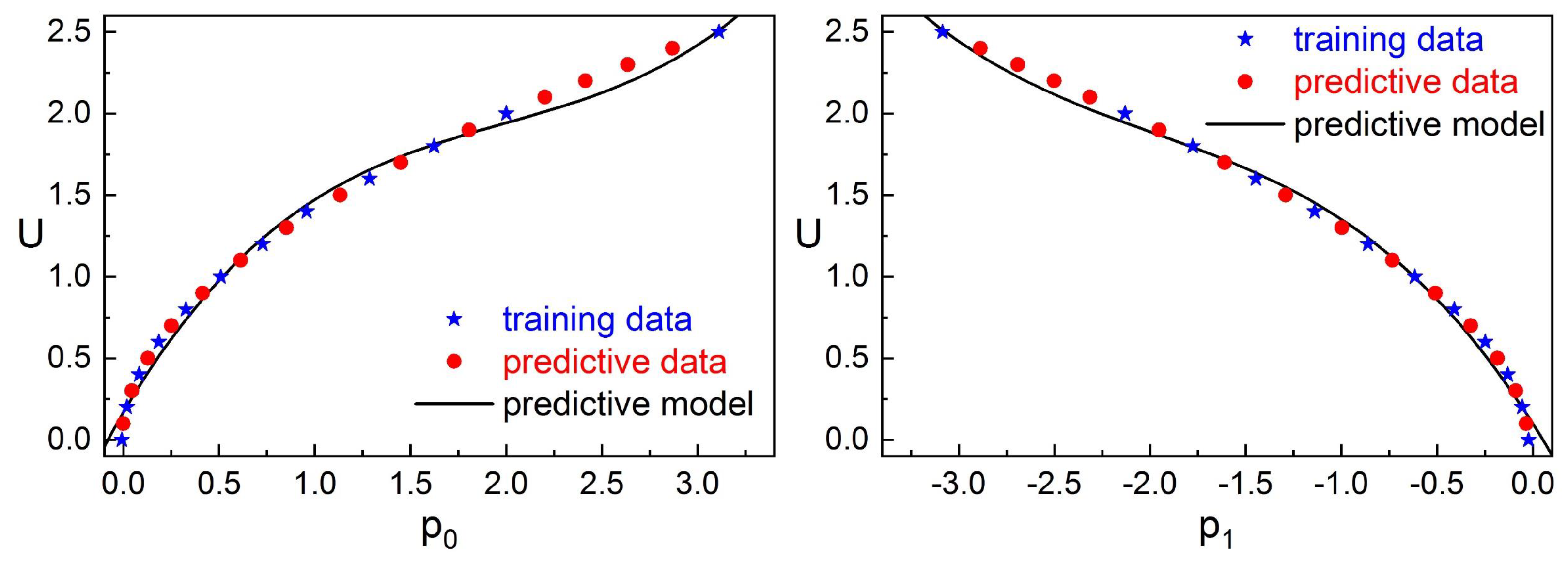As shown in Figure 19, when the spacing $dy$ is $0.2L$, the kinematic pressures differ greatly from that of other spacings at a certain U. This is because the spacing is close, and the impact caused by the swing of two fishes is greater than that of large spacings. However, we found that $p_3^{\prime }$ is monotonic with $dy$ increasing at a certain U as shown in the left of Figure 19. Thus, we can use $p_3^{\prime }$ to judge the spacing.

5.2.2. The Construction and Validation of Judgement Models

Through the results on the left side of Figure 19, we found that, at different inlet flow velocity U, the relationship between $p_3^{\prime }$ and the spacing $dy$ is different. Thus, we also need to use the kinematic pressure $p{1}_0$ or $p{2}_0$, which is insensitive to the spacing as a feature for eliminating the effect of inlet flow velocity. For the presetting appropriate spacing $\Delta d$, we divide the data into two categories: the label is equal to 0 when the current spacing $dy$ is less than $\Delta d$, and the label is equal to 1 when the current spacing $dy$ is greater than $\Delta d$. We used the same neural network structure above. We used the data simulated by settings in Table 4 to train the classification model, and used the data simulated by settings in Table 6 to validate the model. When we construct the model, the input layer contains two features $p_3^{\prime }$ and $p{1}_0$ (which is about equal to $p{2}_0$). However, when we validated the model, we used the kinematic pressures of each fish, and two features in the input layer are $p{1}_{3R}$, $p{1}_0$ or $p{2}_{3L}$, $p{2}_0$. We used several $\Delta d$ to construct the judgement models, and the effects of each fish are shown in

Table 10. The accuracy rate of the judgement models.

$\Delta \mathit{d}$	Accuracy Rate of No. 1 Fish	Accuracy Rate of No. 2 Fish
0.3$L$	$100\%$	$96\%$
0.5$L$	$80\%$	$88\%$
0.7$L$	$88\%$	$84\%$
0.9$L$	$92\%$	$80\%$

.

In this section, we construct some binary classification models to judge the relationship between the current spacing and the presetting appropriate spacing $\Delta d$. Through the results of judging, the robotic fishes can adjust their actions to maintain a stable formation at the appropriate spacing $\Delta d$.

6. Conclusions

In this work, we construct the models for single robotic fish, the tandem formation and the phalanx formation to predict the inlet flow velocity and judge the spacing between individual platforms in the formation. The results show that the best predictive model of the inlet flow velocity for single fish is calculated by the kinematic pressures monitored by sensors at position $x=0.35L$. The predictive models of the inlet flow velocity for the front robotic fish in the tandem formation and two fishes in the phalanx formation are the same as that of single fish calculated by the kinematic pressures at the fish head. The predictive model of the inlet flow velocity for robotic fish at the back in the tandem is calculated by the kinematic pressures monitored by the sensors at position $x=0.35L$, which is different from the best model for single fish. In the tandem formation, only the fish at the back need to know the spacing with the other fish. The spacing is judged by the kinematic pressures monitored by the sensors at position $x=0.15L$. In the phalanx, both fishes need to know the spacing. For the fish on the left, the spacing is judged by the data monitored by the right sensors at position $x=0.15L$. For the right fish, the spacing is judged by the data monitored by the left sensors at position $x=0.15L$. The robotic fishes can know basic environmental information, such as the inlet flow velocity and the spacing between the robotic fish itself and the other fish in the formation through these models. It is useful for maintaining a stable formation to perform more complex tasks without communication. In addition, the results can provide guidance for sensor installation position on the robotic fish surface. In the future, we will further consider more complex formations with more robotic fishes and change the phase difference of fishes swing. We will try to improve the applicability of the predictive and judgement models. To make the simulation closer to reality, we will also consider more control algorithms and cooperate with colleagues who make robots to apply our simulation results to actual robots.