Electrocardiographic Fragmented Activity (II): A Machine Learning Approach to Detection
 ,
,  , and
, and
Abstract
:1. Introduction
2. Background
3. Materials and Methods
3.1. Databases
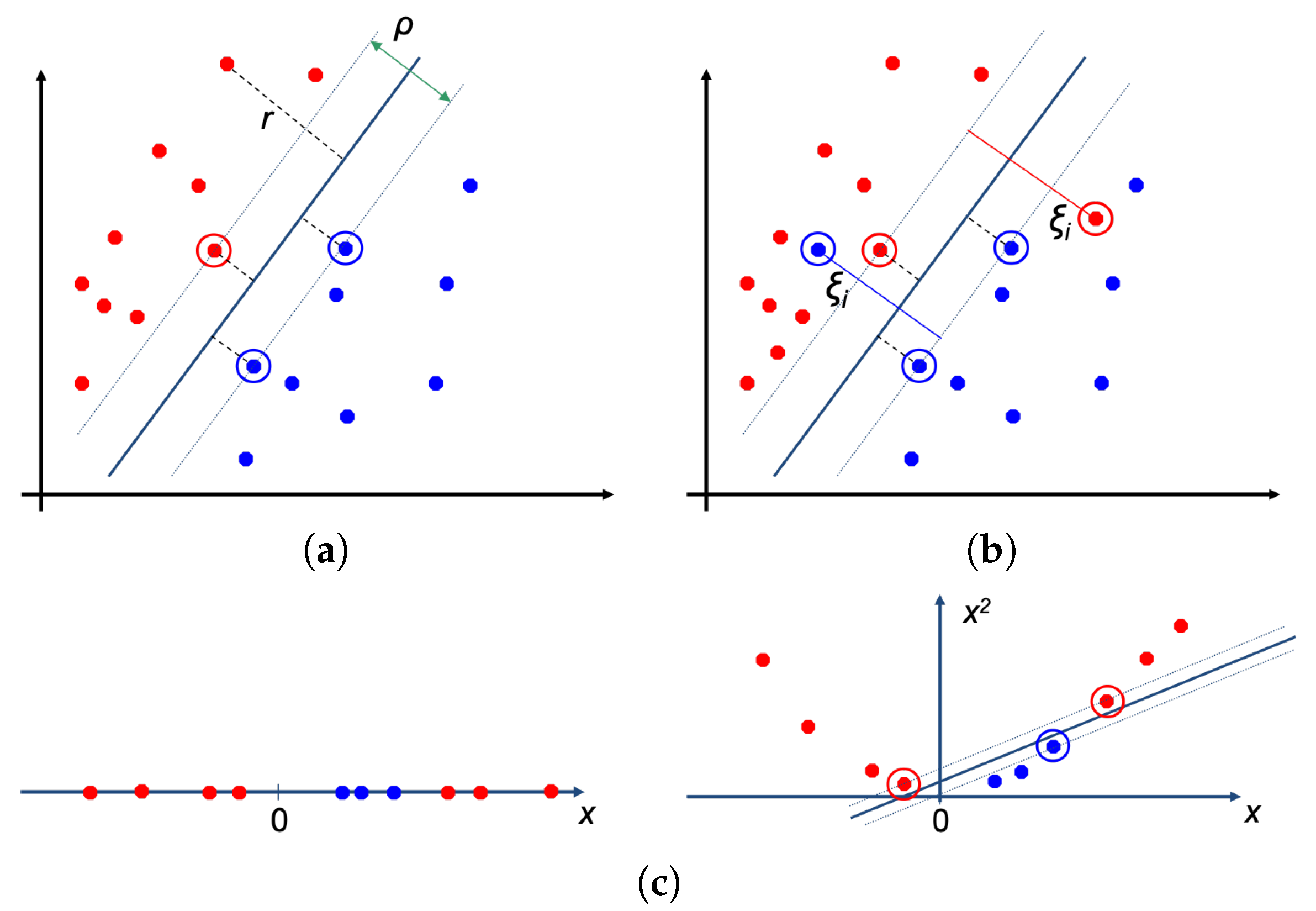
3.2. Classifiers
3.3. Processing and Features Spaces
4. Results
4.1. Fragmentation Detection Based on Linear Models
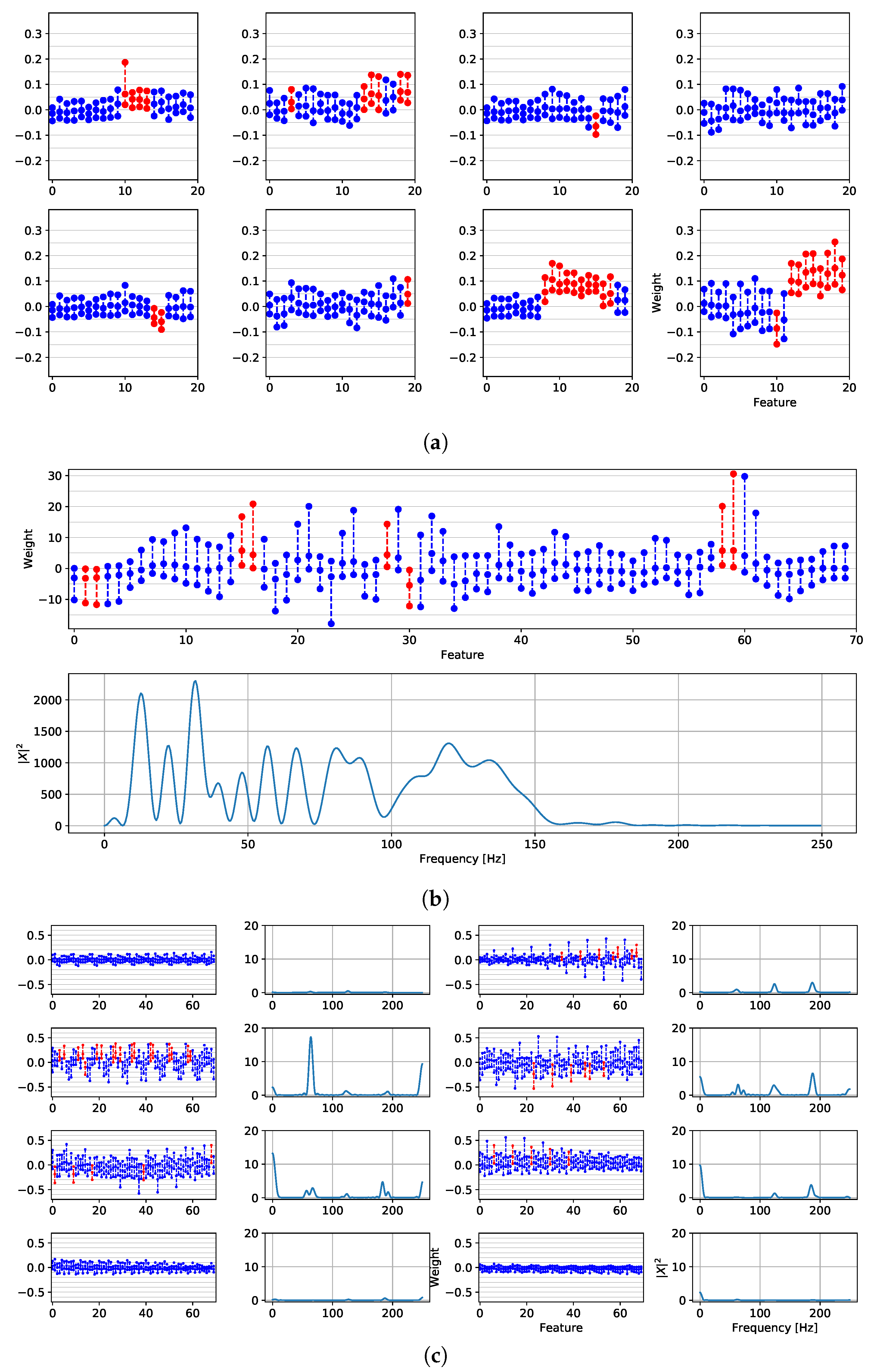
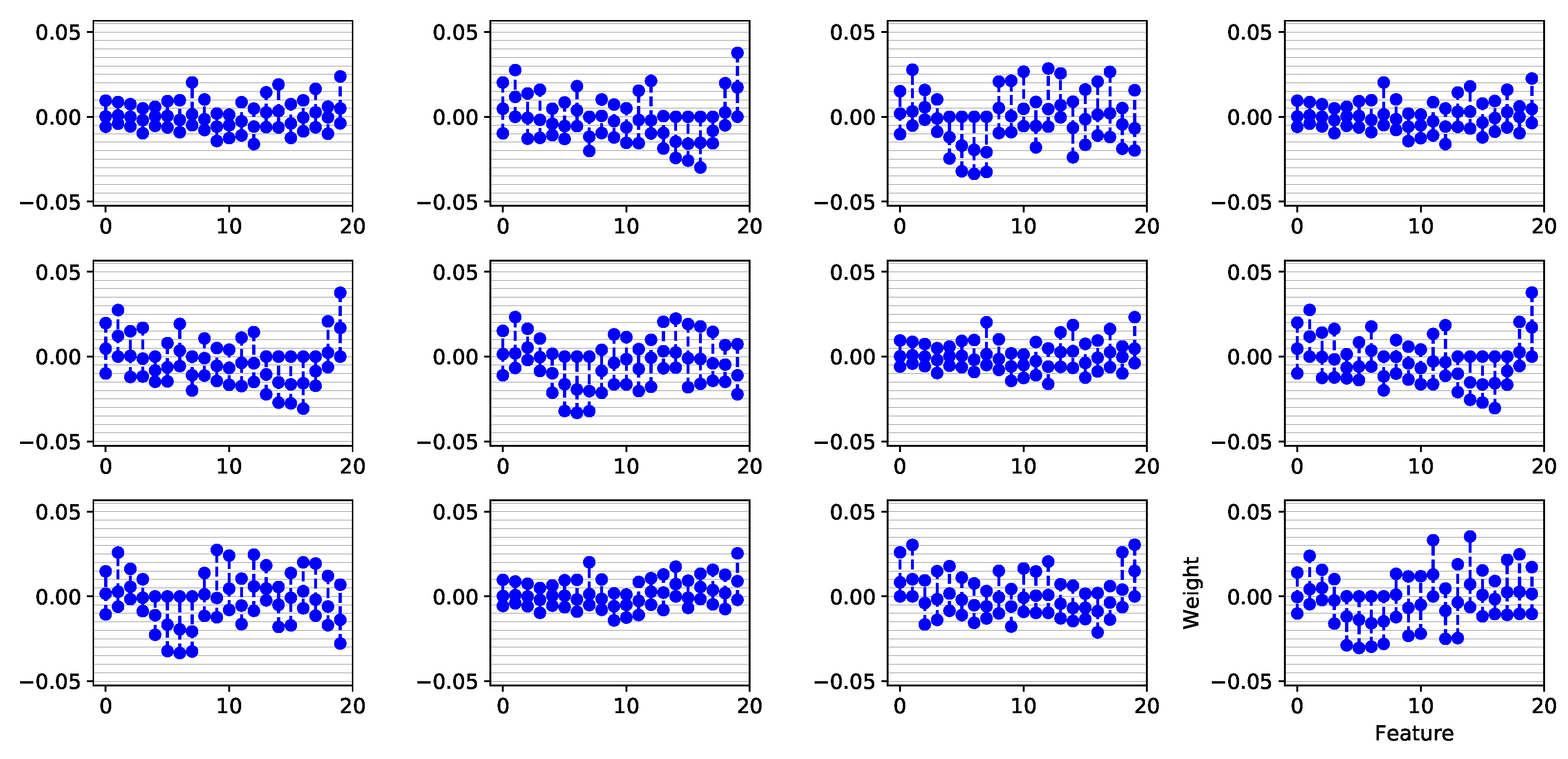
4.2. Features Relevance and New Fragmented Subrogated Model
4.3. Fibrosis Detection Based on Linear Models and Statistical Relevance
4.4. Fragmentation and Fibrosis Detection Based on Non-Linear Models
5. Discussion
Author Contributions
Funding
Conflicts of Interest
References
- Foster, D.B. Twelve-Lead Electrocardiography: Theory and Interpretation, 2nd ed.; Springer: London, UK, 2007. [Google Scholar]
- Lee, D.H.; Park, J.W.; Choi, J.; Rabbi, A.; Fazel-Rezai, R. Automatic Detection of Electrocardiogram ST Segment: Application in Ischemic Disease Diagnosis. Int. J. Adv. Comput. Sci. Appl. 2013, 4. [Google Scholar] [CrossRef]
- Salam, K.A.; Srilakshmi, G. An Algorithm for ECG Analysis of Arrhythmia Detection. In Proceedings of the International Conference on Electrical, Computer and Communication Technologies, Coimbatore, India, 5–7 March 2015; pp. 1–6. [Google Scholar]
- Liu, T.; Song, D.; Dong, J.; Zhu, P.; Liu, J.; Liu, W.; Ma, X.; Zhao, L.; Ling, S. Current Understanding of the Pathophysiology of Myocardial Fibrosis and Its Quantitative Assessment in Heart Failure. Front. Physiol. 2017, 8, 238. [Google Scholar] [CrossRef] [PubMed]
- Basaran, Y.; Tigen, K.; Karaahmet, T.; Isiklar, I.; Cevik, C.; Gurel, E.; Dundar, C.; Pala, S.; Mahmutyazicioglu, K.; Basaran, O. Fragmented QRS Complexes Are Associated with Cardiac Fibrosis and Significant Intraventricular Systolic Dyssynchrony in Nonischemic Dilated Cardiomyopathy Patients with a Narrow QRS Interval. Echocardiography 2011, 28, 62–68. [Google Scholar] [CrossRef] [PubMed]
- Kang, K.W.; Janardhan, A.H.; Jung, K.T.; Lee, H.S.; Lee, M.H.; Hwang, H.J. Fragmented QRS as a Candidate Marker for High-Risk Assessment in Hypertrophic Cardiomyopathy. Heart Rhythm 2014, 11, 1433–1440. [Google Scholar] [CrossRef] [PubMed]
- Konno, T.; Hayashi, K.; Fujino, N.; Oka, R.; Nomura, A.; Nagata, Y.; Hodatsu, A.; Sakata, K.; Furusho, H.; Takamura, M.; et al. Electrocardiographic QRS Fragmentation as a Marker for Myocardial Fibrosis in Hypertrophic Cardiomyopathy. J. Cardiovasc. Electrophysiol. 2015, 26, 1081–1087. [Google Scholar] [PubMed]
- Melgarejo-Meseguer, F.M.; Gimeno-Blanes, F.J.; Salar-Alcaraz, M.E.; Gimeno-Blanes, J.R.; Martínez-Sánchez, J.; García-Alberola, A.; Rojo-Álvarez, J.L. Electrocardiographic Fragmented Activity (I): Physiological Meaning of Multivariate Signal Decompositions. Appl. Sci. 2019. This issue. [Google Scholar]
- Maheshwari, S.; Acharyya, A.; Puddu, P.E.; Mazomenos, E.B.; Leekha, G.; Maharatna, K.; Schiariti, M. An Automated Algorithm for Online Detection of Fragmented QRS and Identification of Its Various Morphologies. J. R. Soc. Interface 2013, 10, 20130761. [Google Scholar] [PubMed]
- Jin, F.; Sugavaneswaran, L.; Krishnan, S.; Chauhan, V.S. Quantification of Fragmented QRS Complex Using Intrinsic Time-Scale Decomposition. Biomed. Signal Process. Control. 2017, 31, 513–523. [Google Scholar] [CrossRef]
- Bono, V.; Mazomenos, E.B.; Chen, T.; Rosengarten, J.A.; Acharyya, A.; Maharatna, K.; Morgan, J.M.; Curzen, N. Development of an Automated Updated Selvester QRS Scoring System Using SWT-based QRS Fractionation Detection and Classification. IEEE J. Biomed. Health Inform. 2014, 18, 193–204. [Google Scholar] [CrossRef] [PubMed]
- Goovaerts, G.; Padhy, S.; Vandenberk, B.; Varon, C.; Willems, R.; Huffel, S.V. A Machine Learning Approach for Detection and Quantification of QRS Fragmentation. IEEE J. Biomed. Health Inform. 2018. [Google Scholar] [CrossRef] [PubMed]
- Gimeno-Blanes, F.J.; Rojo-Álvarez, J.L.; García-Alberola, A.; Gimeno-Blanes, J.R.; Rodríguez-Martínez, A.; Mocci, A.; Flores-Yepes, J.A. Early Prediction of Tilt Test Outcome, with Support Vector Machine Non Linear Classifier, Using ECG, Pressure and Impedance Signals. Comput. Cardiol. 2011, 38, 101–104. [Google Scholar]
- Basar, M.D.; Kotan, S.; Kilic, N.; Akan, A. Morphologic Based Feature Extraction for Arrhythmia Beat Detection. In Proceedings of the Medical Technologies National Congress, Antalya, Turkey, 27–29 October 2016; pp. 1–4. [Google Scholar]
- Rojo-Álvarez, J.L.; García-Alberola, A.; Arenal-Maíz, A.; Piñeiro-Ave, J.; Valdés-Chavarri, M.; Artés-Rodríguez, A. Automatic Discrimination Between Supraventricular and Ventricular Tachycardia using a Multilayer Perceptron in Implantable Cardioverter Defibrillators. Pacing Clin. Electrophysiol. 2002, 25, 1599–1604. [Google Scholar] [CrossRef] [PubMed]
- Bhoi, A.K.; Sherpa, K.S.; Khandelwal, B. Ischemia and Arrhythmia Classification Using Time-Frequency Domain Features of QRS Complex. Procedia Comput. Sci. 2018, 132, 606–613. [Google Scholar] [CrossRef]
- Paing, M.P.; Hamamoto, K.; Tungjitkusolmun, S.; Pintavirooj, C. Automatic Detection and Staging of Lung Tumors using Locational Features and Double-Staged Classifications. Appl. Sci. 2019, 9, 2329. [Google Scholar] [CrossRef]
- Pedregosa, F.; Varoquaux, G.; Gramfort, A.; Michel, V.; Thirion, B.; Grisel, O.; Blondel, M.; Müller, A.; Nothman, J.; Louppe, G.; et al. Scikit-learn: Machine Learning in Python. J. Mach. Learn. Res. 2011, 12, 2825–2830. [Google Scholar]
- Cortes, C.; Vapnik, V. Support-Vector Networks. Mach. Learn. 1995, 20, 273–297. [Google Scholar] [CrossRef]
- Tan, P.N.; Steinbach, M.; Kumar, V. Introduction to Data Mining; Addison-Wesley Longman Publishing Co., Inc.: Boston, MA, USA, 2005. [Google Scholar]
- Cunningham, P.; Delany, S.J. K-Nearest Neighbour Classifiers. Mult. Classif. Syst. 2007, 34, 1–17. [Google Scholar]
- Everss-Villalba, E.; Melgarejo-Meseguer, F.M.; Blanco-Velasco, M.; Gimeno-Blane, F.J.; Sala-Pla, S.; Rojo-Álvarez, J.L.; García-Alberola, A. Noise Maps for Quantitative and Clinical Severity Towards Long-Term ECG Monitoring. Sensors 2017, 17, 2448. [Google Scholar] [CrossRef] [PubMed]
- Melgarejo-Meseguer, F.M.; Everss-Villalba, E.; Gimeno-Blanes, F.J.; Blanco-Velasco, M.; Molins-Bordallo, Z.; Flores-Yepes, J.A.; Rojo-Álvarez, J.L.; García-Alberola, A. On the Beat Detection Performance in Long-Term ECG Monitoring Scenarios. Sensors 2018, 18, 1387. [Google Scholar] [CrossRef] [PubMed]
- Casanez-Ventura, A.; Gimeno-Blanes, F.J.; Rojo-Álvarez, J.L.; Flores-Yepes, J.A.; Gimeno-Blanes, J.R.; Lopez-Ayala, J.M.; García-Alberola, A. QRS Delineation Algorithms Comparison and Model Fine Tuning for Automatic Clinical Classification. In Proceedings of the Computing in Cardiology Conference, Zaragoza, Spain, 22–25 September 2013; pp. 1163–1166. [Google Scholar]
- Melgarejo-Meseguer, F.M.; Gimeno-Blanes, F.J.; Rojo-Álvarez, J.L.; Salar-Alcaraz, M.; Gimeno-Blanes, J.R.; García-Alberola, A. Cardiac Fibrosis Detection Applying Machine Learning Techniques to Standard 12-Lead ECG. In Proceedings of the Computing in Cardiology Conference, Maastricht, The Netherlands, 23–26 September 2018; Volume 45. [Google Scholar]
- Yerushalmy, J. Statistical Problems in Assessing Methods of Medical Diagnosis, with Special Reference to X-Ray Techniques. Public Health Rep. 1947, 62, 1432–1449. [Google Scholar] [CrossRef] [PubMed]
- Whitaker, B.; Rizwan, M.; Aydemir, B.; Rehg, J.; Anderson, D. AF Classification from ECG Recording Using Feature Ensemble and Sparse Coding. In Proceedings of the Computing in Cardiology Conference, Rennes, France, 24–27 September 2017. [Google Scholar]
- Efron, B.; Tibshirani, R.J. An Introduction to the Bootstrap; CRC Press: London, UK, 1994. [Google Scholar]


| Classifier | Input Space | Signal Selection | Sen | Spe | PPV | NPV | Acc |
|---|---|---|---|---|---|---|---|
| NuSVM | Statistics + 3PCA | Non-normalized Beat | 0.70 | 0.75 | 0.76 | 0.69 | 0.73 |
| NuSVM | Statistics + 3PCA | Normalized Beat | 0.70 | 0.81 | 0.80 | 0.71 | 0.75 |
| NuSVM | Statistics + 3PCA | Non-normalized QRS | 0.76 | 0.88 | 0.87 | 0.77 | 0.82 |
| NuSVM | Statistics + PCA | Normalized QRS | 0.75 | 0.90 | 0.89 | 0.76 | 0.82 |
| CSVM | Statistics + ICA | Non-normalized Beat | 0.78 | 0.63 | 0.70 | 0.72 | 0.71 |
| CSVM | Statistics + PCA | Normalized Beat | 0.65 | 0.88 | 0.85 | 0.69 | 0.76 |
| CSVM | Statistics + ICA | Non-normalized QRS | 0.76 | 0.79 | 0.80 | 0.75 | 0.78 |
| CSVM | Statistics + PCA | Normalized QRS | 0.70 | 0.86 | 0.85 | 0.72 | 0.78 |
| Classifier | Input Space | Signal Selection | Sen | Spe | PPV | NPV | Acc |
|---|---|---|---|---|---|---|---|
| NuSVM | Statistics + 8-Ld | Non-normalized Beat | 0.55 | 0.73 | 0.67 | 0.63 | 0.64 |
| NuSVM | Concat + 8-Ld | Normalized Beat | 0.74 | 0.58 | 0.63 | 0.70 | 0.66 |
| NuSVM | Statistics + 12-Ld | Non-normalized QRS | 0.65 | 0.71 | 0.67 | 0.69 | 0.68 |
| NuSVM | Statistics + 12-Ld | Normalized QRS | 0.70 | 0.65 | 0.69 | 0.71 | 0.68 |
| CSVM | Sum + 8-Ld | Non-normalized Beat | 0.59 | 0.75 | 0.69 | 0.65 | 0.67 |
| CSVM | Concat + 8-Ld | Normalized Beat | 0.67 | 0.62 | 0.63 | 0.66 | 0.64 |
| CSVM | Concat + 8-Ld | Non-normalized QRS | 0.61 | 0.75 | 0.69 | 0.68 | 0.68 |
| CSVM | Sum + 8-Ld | Normalized QRS | 0.54 | 0.71 | 0.63 | 0.63 | 0.63 |
| Classifier | Signal Selection | Input Space | Accuracy | Classifier | Signal Selection | Input Space | Accuracy | Classifier | Signal Selection | Input Space | Accuracy |
|---|---|---|---|---|---|---|---|---|---|---|---|
| C-SVM | Normalized QRS | Stats + PCA | 0.79 | C-SVM | Non-normalized QRS | Stats + 3PCA | 0.77 | C-SVM | Normalized QRS | Sum + 8 Ld | 0.91 |
| Nu-SVM | Non-normalized beat | Stats + ICA | 0.78 | Nu-SVM | Non-normalized QRS | Stats + 3PCA | 0.78 | Nu-SVM | Normalized QRS | Sum + 8 Ld | 0.91 |
| KNN | Non-normalized QRS | Stats +PCA | 0.65 | KNN | Normalized QRS | Stats + PCA | 0.72 | KNN | Non-normalized QRS | Stats + 8 Ld | 0.79 |
| MLP | Non-normalized QRS | Stats + ICA | 0.78 | MLP | Non-normalized QRS | Stats + ICA | 0.78 | MLP | Normalized Beat | Stats + 8 Ld | 0.78 |
| DT | Normalized QRS | Stats + 8Ld | 0.81 | DT | Non-normalized QRS | Stats + PCA | 0.78 | DT | Non-normalized QRS | Stats + 12 Ld | 0.79 |
| NB | Non-normalized QRS | Stats +PCA | 0.83 | NB | Non-normalized QRS | Stats + PCA | 0.83 | NB | Normalized QRS | Stats + 8 Ld | 0.79 |
| (a) | (b) | (c) | |||||||||
| Classifier | Signal Selection | Input Space | Accuracy |
|---|---|---|---|
| C-SVM | Normalized QRS | Sum + 8 Ld | 0.68 |
| -SVM | Normalized QRS | Sum + 8 Ld | 0.63 |
| KNN | Non-normalized QRS | Stats + 8 Ld | 0.65 |
| MLP | Non-normalized QRS | Stats + 12 Ld | 0.63 |
| DT | Non-normalized QRS | Stats + 8 Ld | 0.61 |
| NB | Non-normalized QRS | Stats + 8 Ld | 0.70 |
| Data Base | Classifier | Signal Selection | Input Space | Sen | Spe | PPV | NPV | Acc |
|---|---|---|---|---|---|---|---|---|
| Sfrag | Linear -SVM | Normalized QRS | Stats + PCA | 0.730 | 0.772 | 0.780 | 0.721 | 0.750 |
| NB | Non-normalized QRS | Stats + PCA | 0.778 | 0.965 | 0.961 | 0.797 | 0.867 | |
| SWfrag | Linear -SVM | Normalized QRS | Stats + PCA | 0.698 | 0.860 | 0.846 | 0.721 | 0.775 |
| NB | Non-normalized QRS | Stats + PCA | 0.762 | 0.895 | 0.889 | 0.773 | 0.825 | |
| FHCM | Linear -SVM | Normalized Beat | PowSum + RegPCA | 0.733 | 0.941 | 0.917 | 0.800 | 0.844 |
| RBF CSVM | Normalized QRS | Sum + 8 Ld | 0.941 | 0.875 | 0.889 | 0.933 | 0.909 | |
| HCM | Linear -SVM | Non-normalized QRS | Stats + 12 Ld | 0.649 | 0.714 | 0.673 | 0.692 | 0.683 |
| NB | Non-normalized QRS | Stats + 8 Ld | 0.474 | 0.905 | 0.818 | 0.655 | 0.700 |
© 2019 by the authors. Licensee MDPI, Basel, Switzerland. This article is an open access article distributed under the terms and conditions of the Creative Commons Attribution (CC BY) license (http://creativecommons.org/licenses/by/4.0/).
Share and Cite
Melgarejo-Meseguer, F.-M.; Gimeno-Blanes, F.-J.; Salar-Alcaraz, M.-E.; Gimeno-Blanes, J.-R.; Martínez-Sánchez, J.; García-Alberola, A.; Rojo-Álvarez, J.L. Electrocardiographic Fragmented Activity (II): A Machine Learning Approach to Detection. Appl. Sci. 2019, 9, 3565. https://doi.org/10.3390/app9173565
Melgarejo-Meseguer F-M, Gimeno-Blanes F-J, Salar-Alcaraz M-E, Gimeno-Blanes J-R, Martínez-Sánchez J, García-Alberola A, Rojo-Álvarez JL. Electrocardiographic Fragmented Activity (II): A Machine Learning Approach to Detection. Applied Sciences. 2019; 9(17):3565. https://doi.org/10.3390/app9173565
Chicago/Turabian StyleMelgarejo-Meseguer, Francisco-Manuel, Francisco-Javier Gimeno-Blanes, María-Eladia Salar-Alcaraz, Juan-Ramón Gimeno-Blanes, Juan Martínez-Sánchez, Arcadi García-Alberola, and José Luis Rojo-Álvarez. 2019. "Electrocardiographic Fragmented Activity (II): A Machine Learning Approach to Detection" Applied Sciences 9, no. 17: 3565. https://doi.org/10.3390/app9173565
APA StyleMelgarejo-Meseguer, F.-M., Gimeno-Blanes, F.-J., Salar-Alcaraz, M.-E., Gimeno-Blanes, J.-R., Martínez-Sánchez, J., García-Alberola, A., & Rojo-Álvarez, J. L. (2019). Electrocardiographic Fragmented Activity (II): A Machine Learning Approach to Detection. Applied Sciences, 9(17), 3565. https://doi.org/10.3390/app9173565