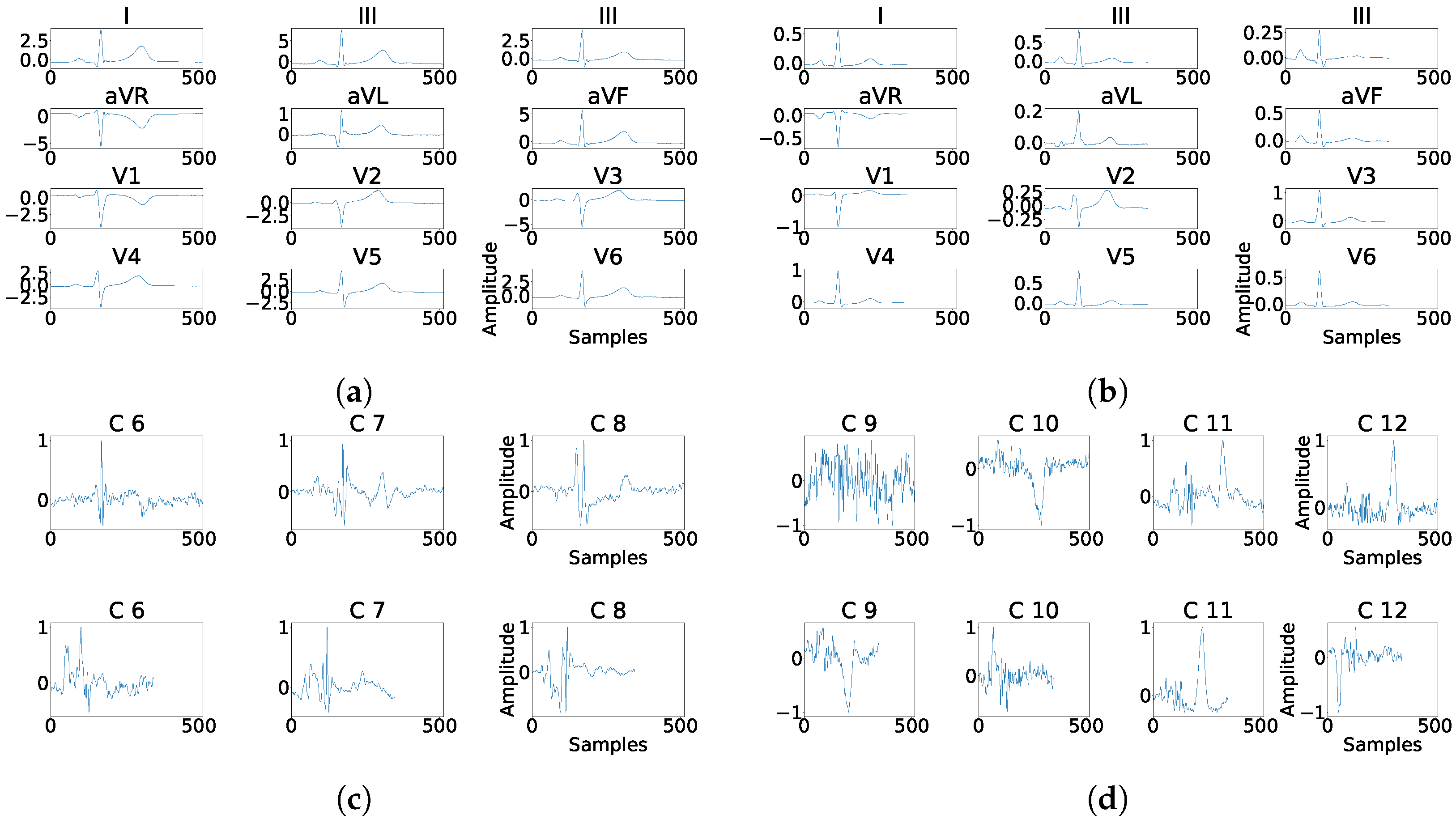
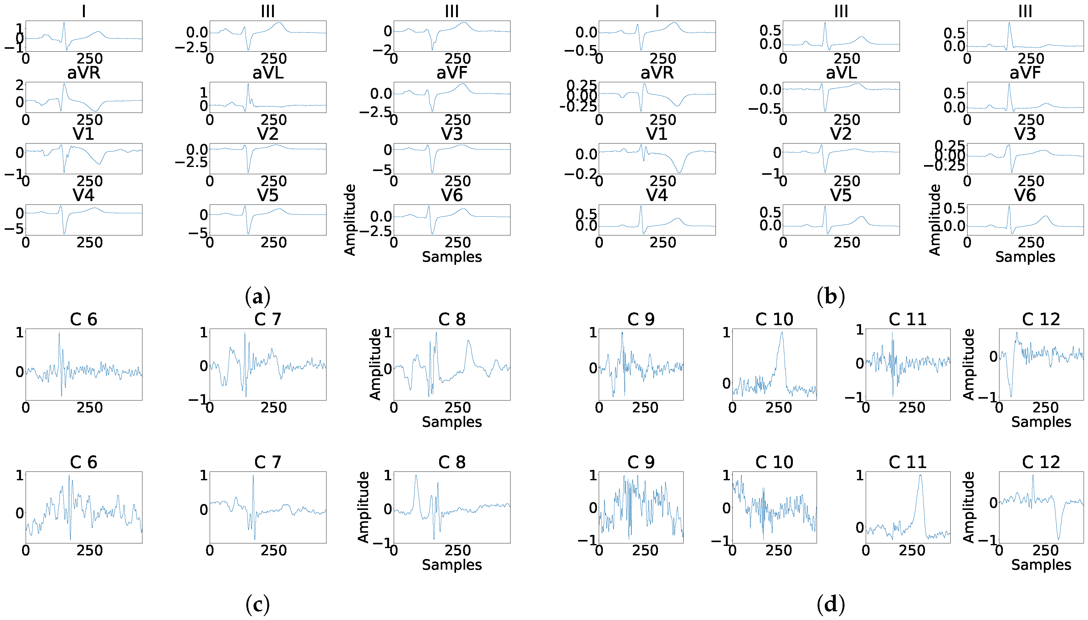
Figure 1.
Example for each type of used register in this work. (a) Example of a beat without fragmentation. (b) Example of a fragmented beat. (c) Example of a beat from control patient. (d) Example of a synthetically fragmented beat.
Figure 1.
Example for each type of used register in this work. (a) Example of a beat without fragmentation. (b) Example of a fragmented beat. (c) Example of a beat from control patient. (d) Example of a synthetically fragmented beat.
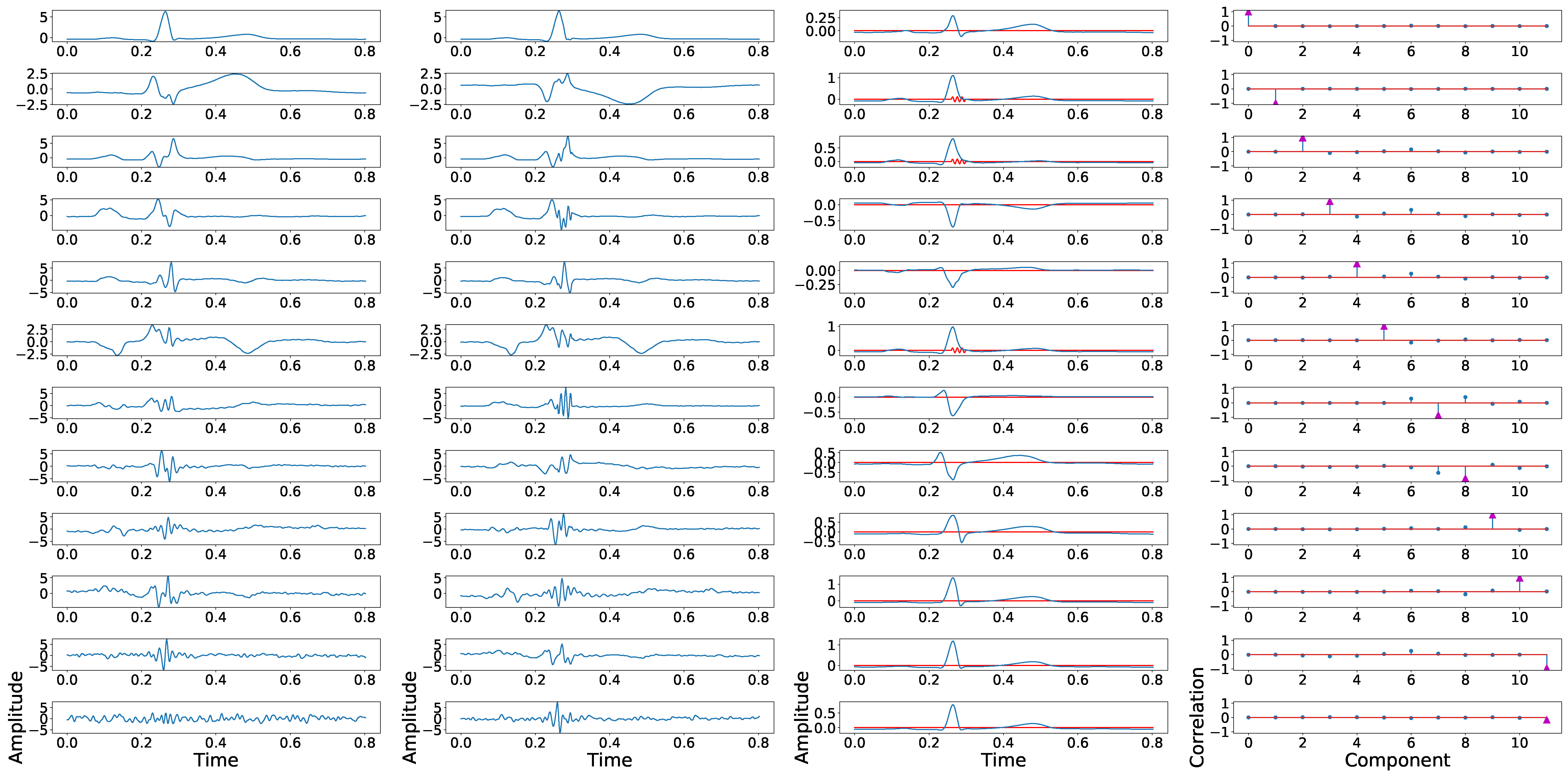
Figure 2.
Example of principal components position swapping in twelve-lead PCA model. The first column shows the principal components of a control ECG, the second column shows the principal components of a synthetically fragmented replication of the previous control ECG, the third column shows the control ECG in blue, and the fragmented wave added in red. The fourth column shows the PCC between the principal component of control ECG with each component of synthetically fragmented.
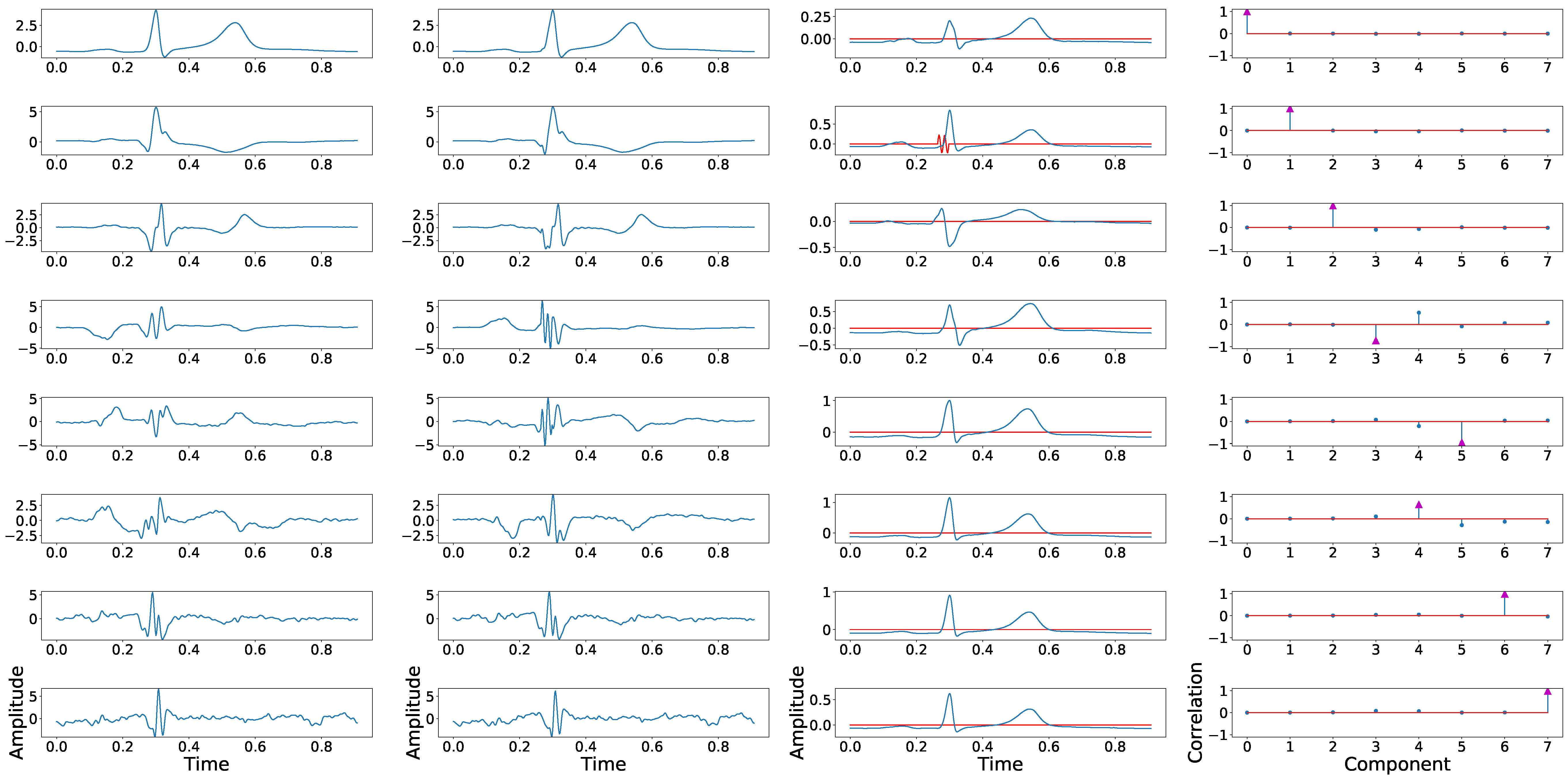
Figure 3.
Example of principal component position swapping in 8 independent leads configuration. The first column shows the principal components associated with the control ECG. The second column shows the principal components derived from the synthetically fragmented replication of the control ECG. The third column shows the original signal in blue and the fragmented wave in red. The fourth column shows the PCCs between the component of the control signal and each component of the fragmented signal.
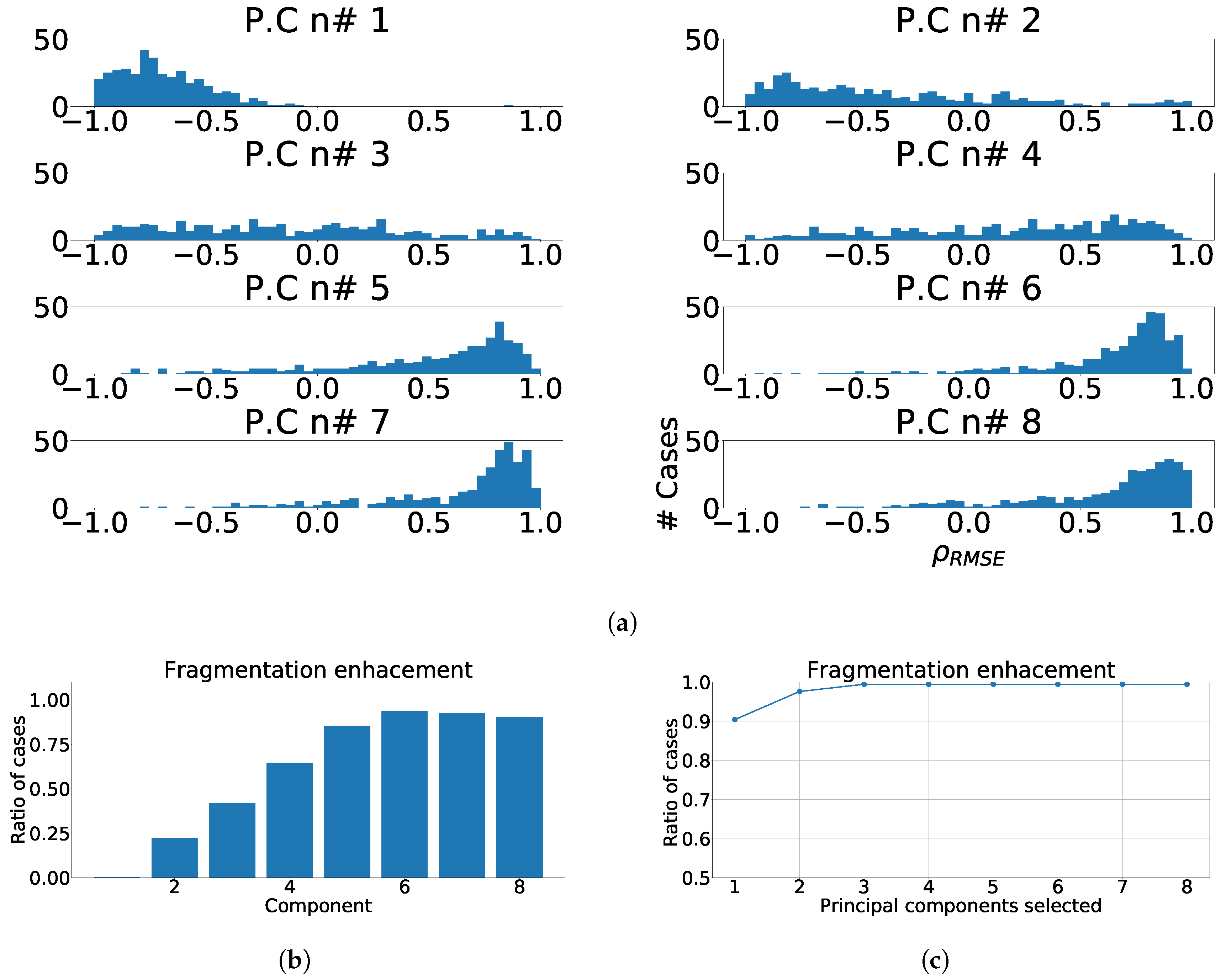
Figure 4.
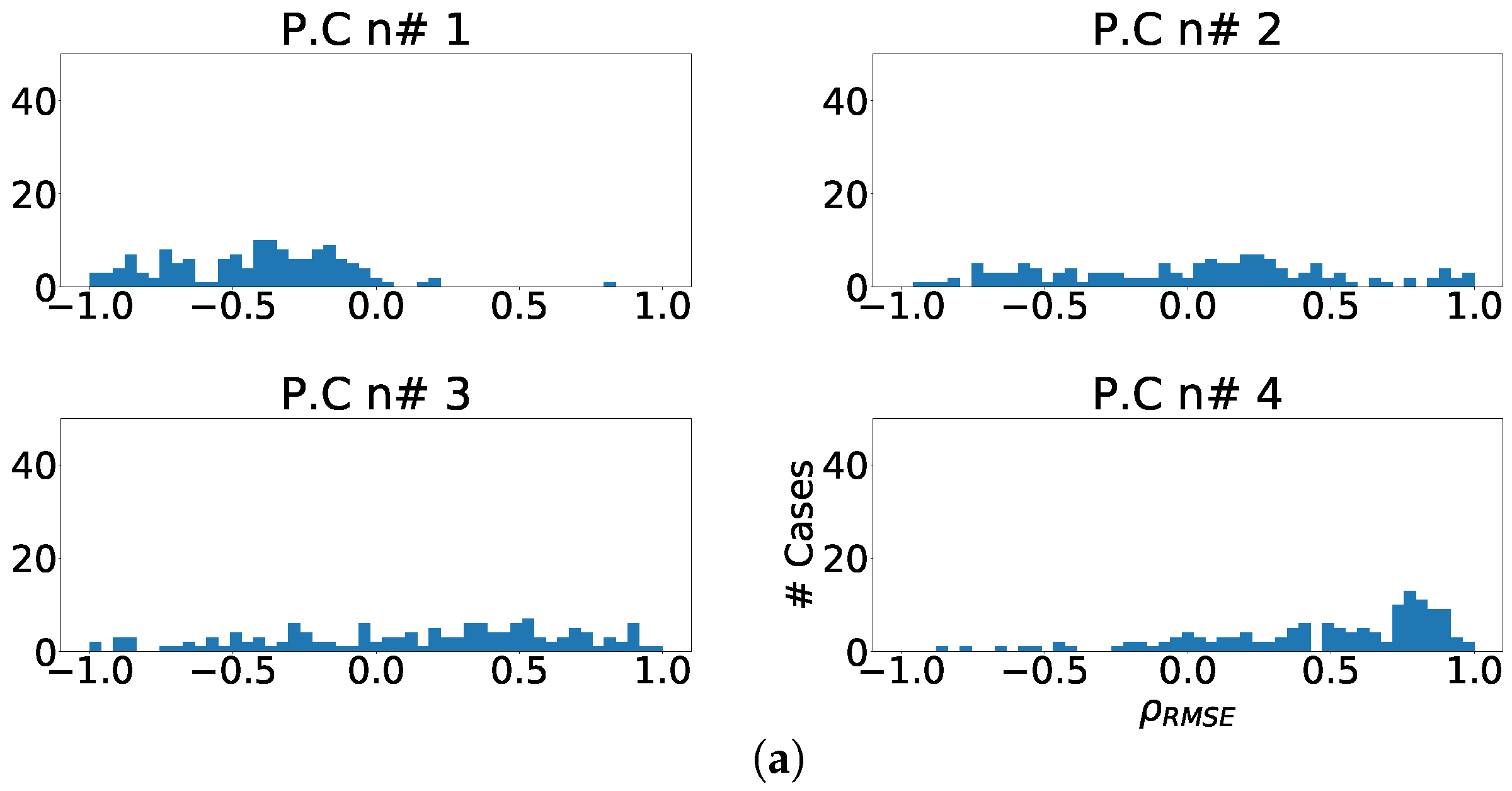
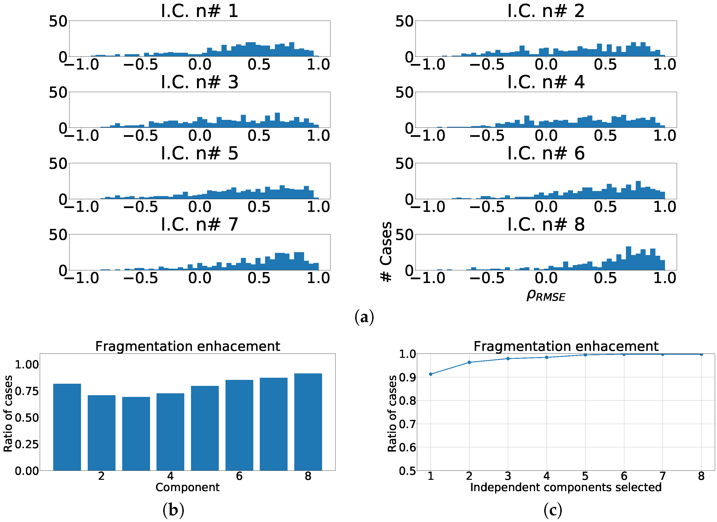
Measurements of fragmentation enhancement using PCA over independent leads. (a) Distribution of coefficient for each component, values higher than 0 represent fragmented wave enhancement. (b) Enhancement ratio for each component. (c) Joint enhancement ratio.
Figure 4.
Measurements of fragmentation enhancement using PCA over independent leads. (a) Distribution of coefficient for each component, values higher than 0 represent fragmented wave enhancement. (b) Enhancement ratio for each component. (c) Joint enhancement ratio.
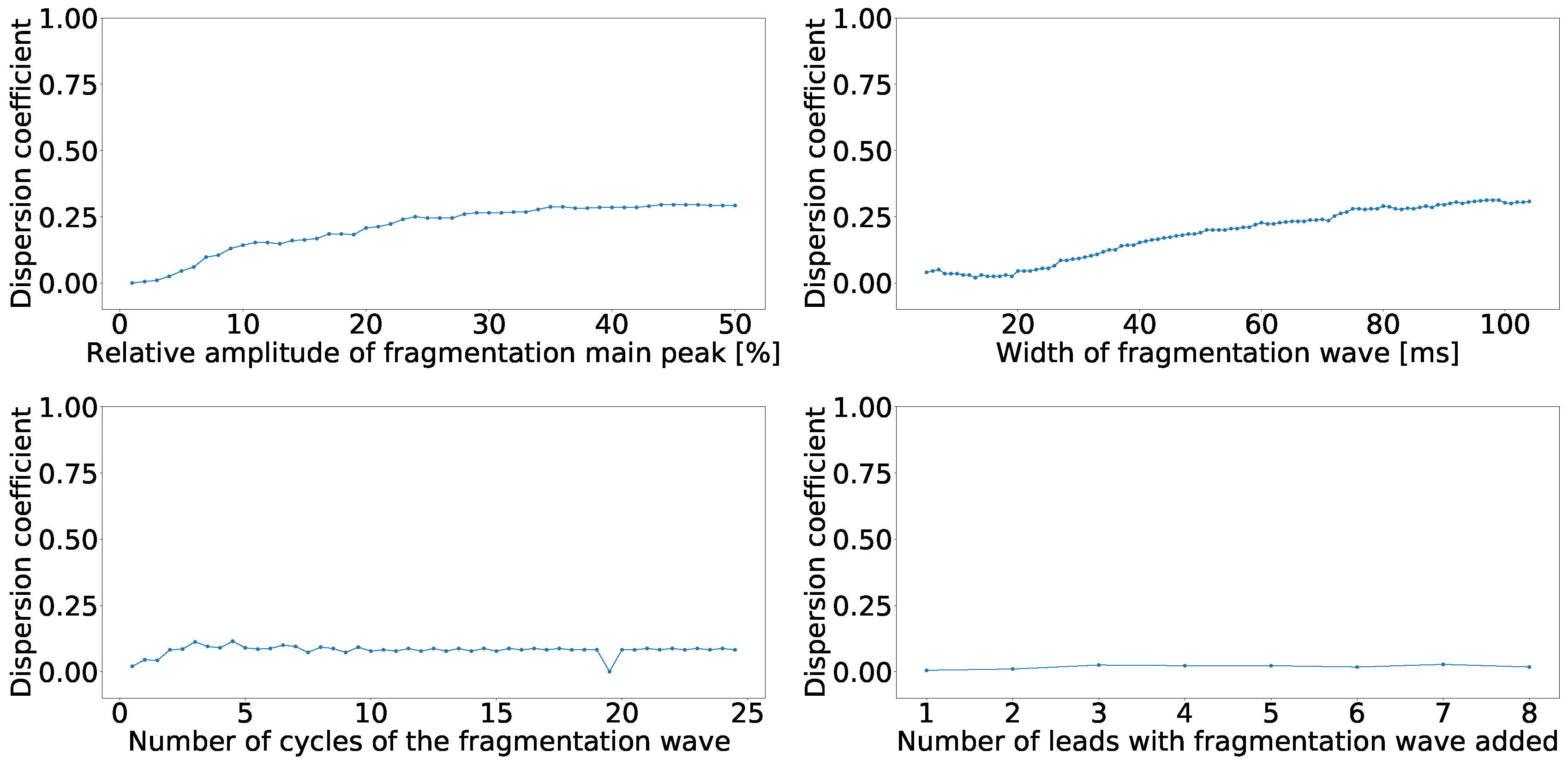
Figure 5.
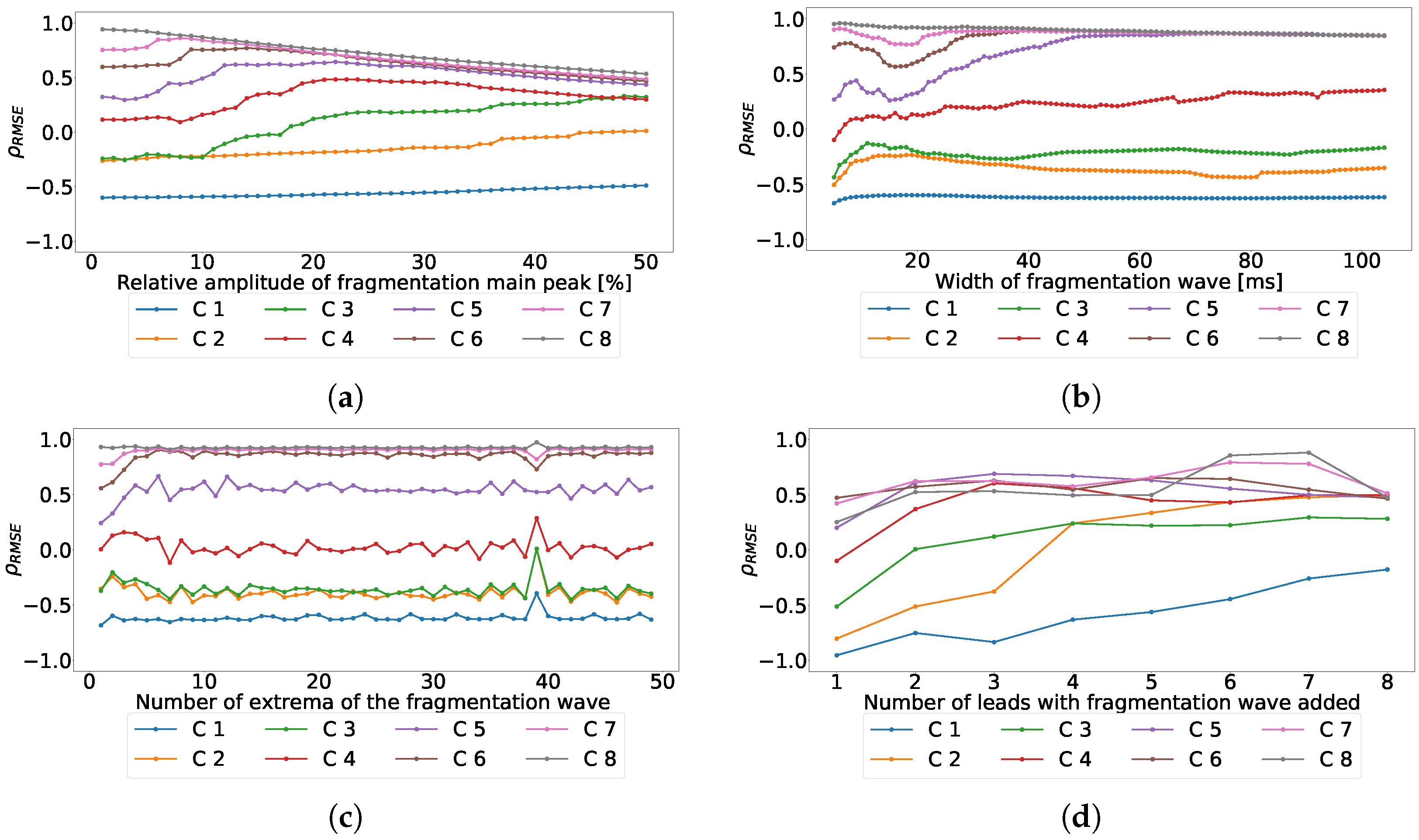
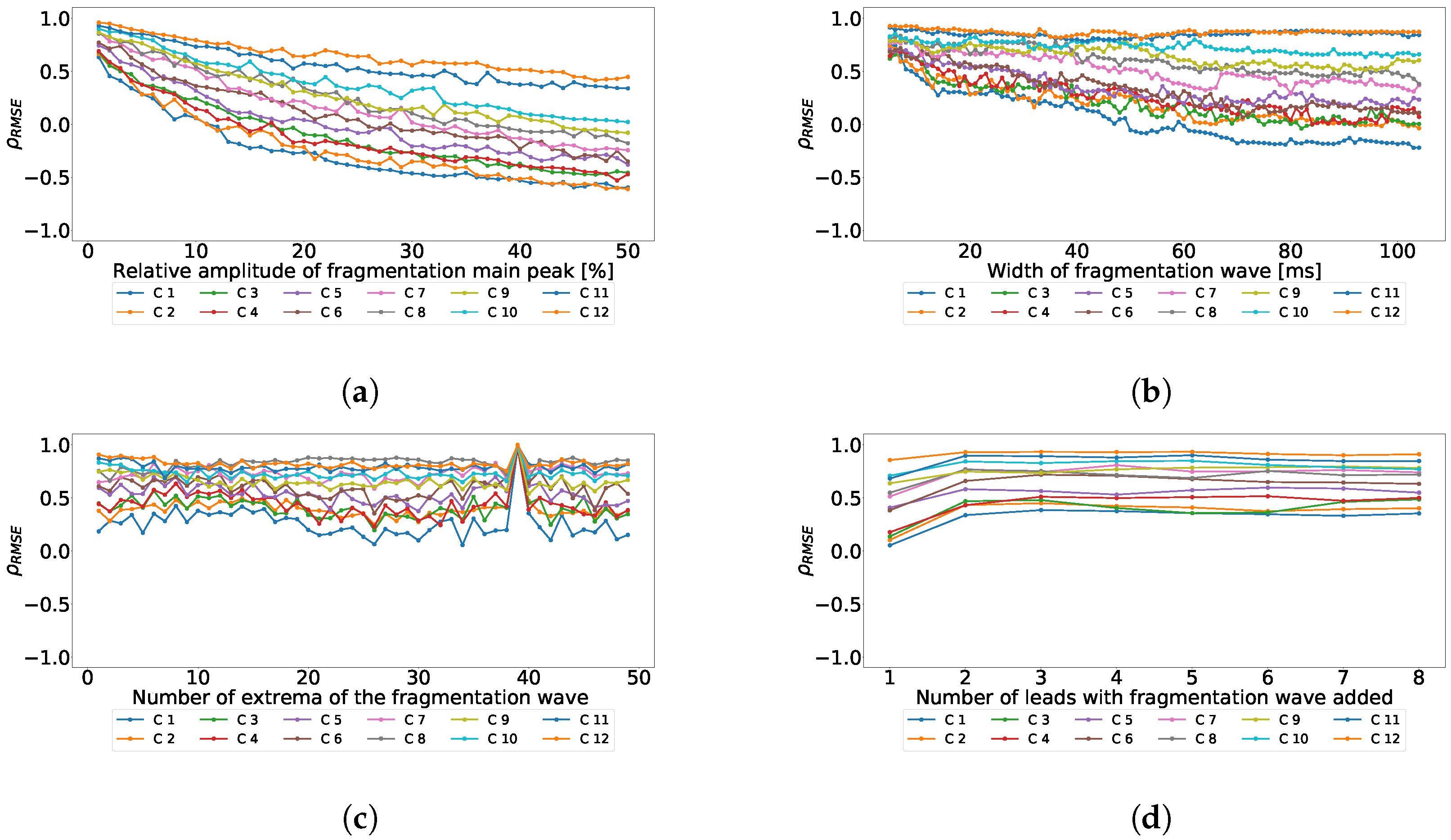
Dispersion coefficient against the fragmented wave amplitude (upper left), fragmented wave width (upper right), fragmented wave number of cycles (lower left), and number of affect lead (lower right) for independent-lead PCA model.
Figure 5.
Dispersion coefficient against the fragmented wave amplitude (upper left), fragmented wave width (upper right), fragmented wave number of cycles (lower left), and number of affect lead (lower right) for independent-lead PCA model.
Figure 6.
Effect of the different parameters of the subrogated fragmented wave over the coefficient for independent-lead PCA model. Values lower than 0 correspond with RMSE higher in the ECG than in the principal components, values higher than 0 correspond with RMSE higher in principal components than in the ECG. (a) Effect of the fragmented wave amplitude, (b) effect of the fragmented wave width, (c) effect of the cycle number of fragmented waves, and (d) effect of the number of affected leads.
Figure 7.
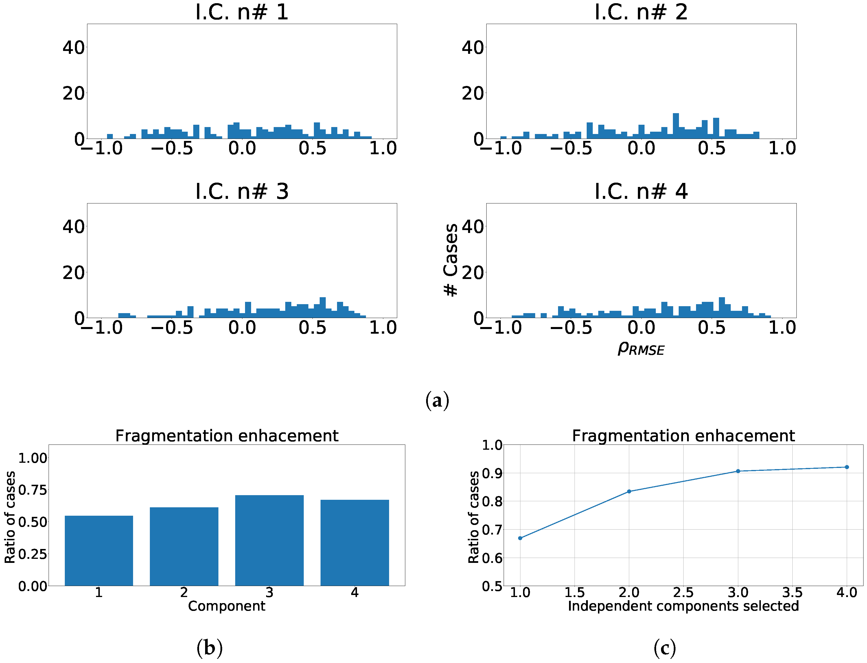
Different measurements for PCA over antero-septal heart region. (a) Distribution of coefficient for each independent component, values lower than zero represents cases where the RMSE measured over the ECG is greater than RMSE measured over the independent component. (b) Ratio of fragmentation wave enhancement for each independent component, this ratio is computed as cases where the value is greater than zero. (c) Cumulative ratio of fragmentation wave enhancement, this ratio is computed by joining the results of isolated independent components.
Figure 8.
Different measurements for PCA over lateral heart region. (a) Distribution of coefficient for each independent component, values lower than zero represents cases where the RMSE measured over the ECG is greater than RMSE measured over the independent component. (b) Ratio of fragmentation wave enhancement for each independent component, this ratio is computed as cases where the value is greater than zero. (c) Cumulative ratio of fragmentation wave enhancement, this ratio is computed by joining the results of isolated independent components.
Figure 9.
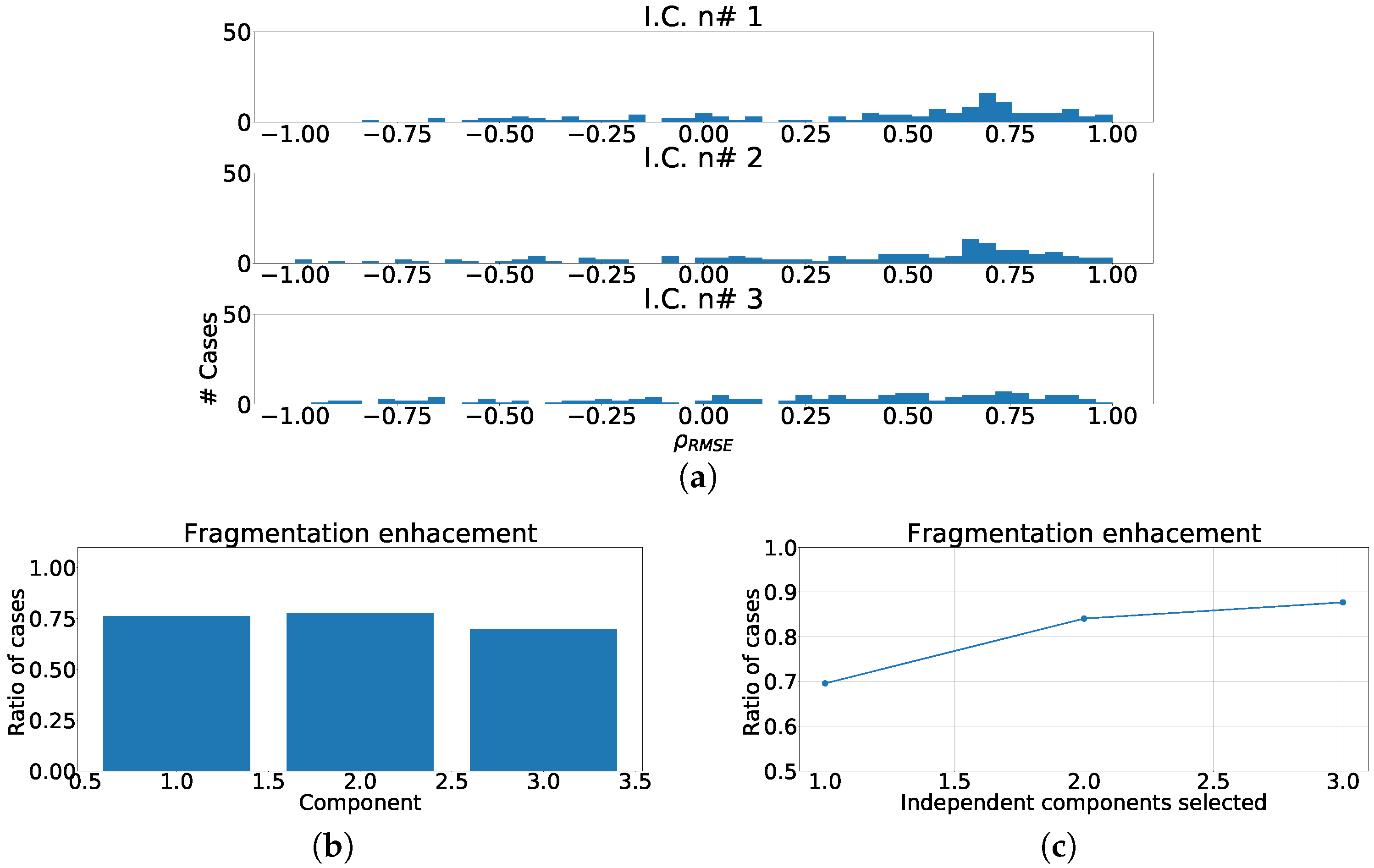
Different measurements for PCA over inferior heart region. (a) Distribution of coefficient for each independent component, values lower than zero represents cases where the RMSE measured over the ECG is greater than RMSE measured over the independent component. (b) Ratio of fragmentation wave enhancement for each independent component, this ratio is computed as cases where the value is greater than zero. (c) Cumulative ratio of fragmentation wave enhancement, this ratio is computed by joining the results of isolated independent components.
Figure 10.
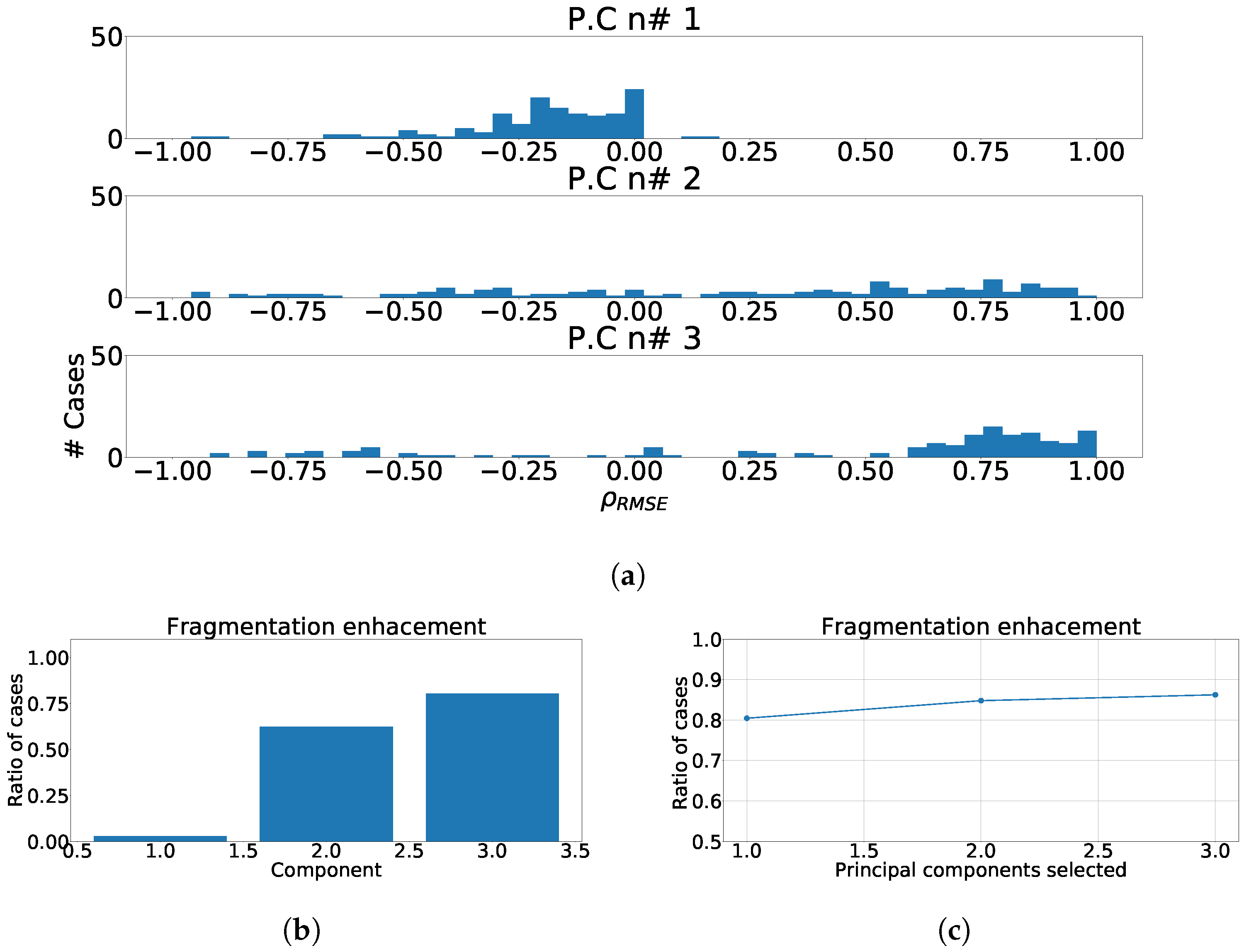
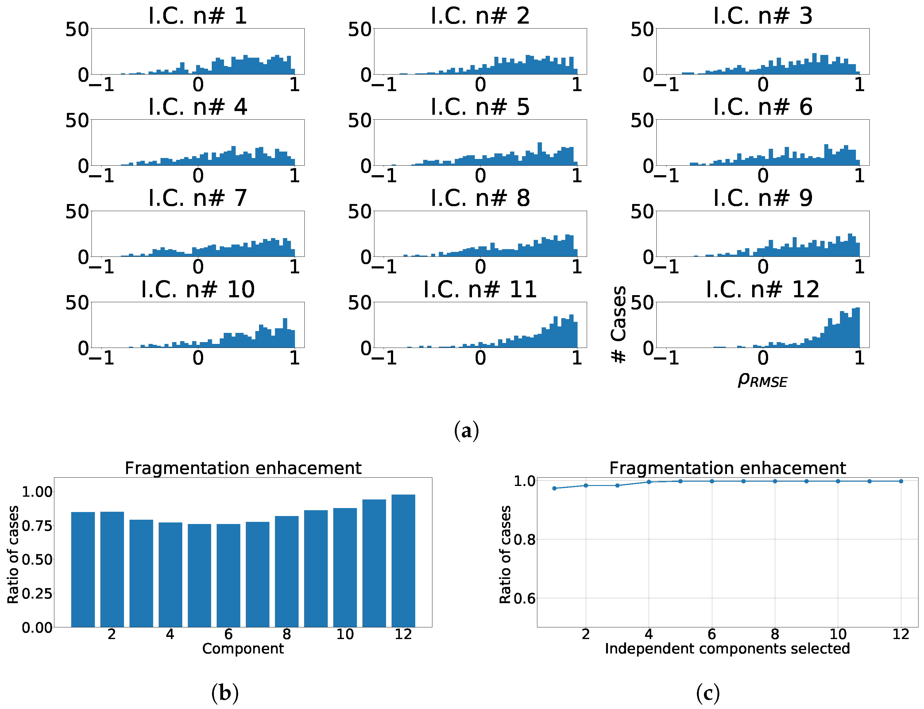
Different measurements for ICA applied over twelve-lead ECG. (a) Distribution of coefficient for each independent component, values lower than zero represents values of RMSE over ECG greater than values of RMSE over ICA output. (b) Ratio of fragmentation wave enhancement for each independent component, ratio of cases where the coefficient is greater than zeros. (c) Cumulative ratio of fragmentation wave enhancement, this ratio is computed by joining the results of isolated independent components.
Figure 11.
Effect of the different parameters of the subrogated fragmented wave over the coefficient using the ICA twelve-lead model. Values lower than 0 correspond with RMSE higher in the ECG than in the principal components, values higher than 0 correspond with RMSE higher in principal components than in the ECG. (a) Effect of the fragmented wave amplitude; (b) Effect of the fragmented wave width; (c) Effect of the cycle number of fragmented waves; (d) Effect of the number of affected leads.
Figure 12.
Different measurements for the antero-septal region of the heart with ICA model. The panel (a) shows the distribution of coefficient for each independent component, values lower than zero represents cases where the RMSE measured over the ECG is greater than RMSE measured over the independent component. Panel (b) shows the ratio of fragmentation wave enhancement for each independent component, this ratio is computed as cases where the value is greater than zero. Panel (c) shows the cumulative ratio of fragmentation wave enhancement, this ratio is computed by joining the results of isolated independent components.
Figure 13.
Different measurements for the lateral region of the heart with ICA model. (a) Distribution of coefficient for each independent component, values lower than zero represents cases where the RMSE measured over the ECG is greater than RMSE measured over the independent component. (b) Ratio of fragmentation wave enhancement for each independent component, this ratio is computed as cases where the value is greater than zero. (c) Cumulative ratio of fragmentation wave enhancement, this ratio is computed by joining the results of isolated independent components.
Figure 14.
Different measurements for the inferior region of the heart with ICA model. (a) Distribution of coefficient for each independent component, values lower than zero represents cases where the RMSE measured over the ECG is greater than RMSE measured over the independent component. (b) Ratio of fragmentation wave enhancement for each independent component, this ratio is computed as cases where the value is greater than zero. (c) Cumulative ratio of fragmentation wave enhancement, this ratio is computed by joining the results of isolated independent components.
Figure 15.
Different measurements for ICA over independent leads model. (a) Distribution of coefficient for each independent component, values lower than zero represents cases where the RMSE measured over the ECG is greater than RMSE measured over the independent component. (b) ratio of fragmentation wave enhancement for each independent component, this ratio is computed as cases where the value is greater than zero. (c) Cumulative ratio of fragmentation wave enhancement, this ratio is computed by joining the results of isolated independent components.
Figure 16.
Example of fragmentation wave enhancement over real fragmented case. (a) Beat templates for each lead of real fragmented case. (b) Beat templates for each lead of control case. (c) Results of the best PCA method for the real fragmented case, in top subpanels and control case in bottom panels. (d) Results of the best ICA method for the real fragmented case, in top subpanels and for the control case in bottom panels.
Figure 17.
Example of fragmentation wave enhancement over real fragmented case. (a) Beat templates for each lead of real fragmented case. (b) Beat templates for each lead of control case. (c) Results of the best PCA method for the real fragmented case, in top subpanels and control case in bottom panels. (d) Results of the best ICA method for the real fragmented case, in top subpanels and for the control case in bottom panels.
Figure 18.
Example of fragmentation wave enhancement over real fragmented case. (a) Beat templates for each lead of real fragmented case. (b) Beat templates for each lead of control case. (c) Results of the best PCA method for the real fragmented case, in top subpanels and control case in bottom panels. (d) Results of the best ICA method for the real fragmented case, in top subpanels and for the control case in bottom panels.
Figure 19.
Example of fragmentation wave enhancement over real fragmented case. (a) Beat templates for each lead of real fragmented case. (b) Beat templates for each lead of control case. (c) Results of the best PCA method for the real fragmented case, in top subpanels and control case in bottom panels. (d) Results of the best ICA method for the real fragmented case, in top subpanels and for the control case in bottom panels.
Figure 20.
Example of fragmentation wave enhancement over real fragmented case. (a) Beat templates for each lead of real fragmented case, (b) beat templates for each lead of control case, (c) results of the best PCA method for the real fragmented case, in top subpanels and control case in bottom panels, and (d) results of the best ICA method for the real fragmented case, in top subpanels and control case in bottom panels.
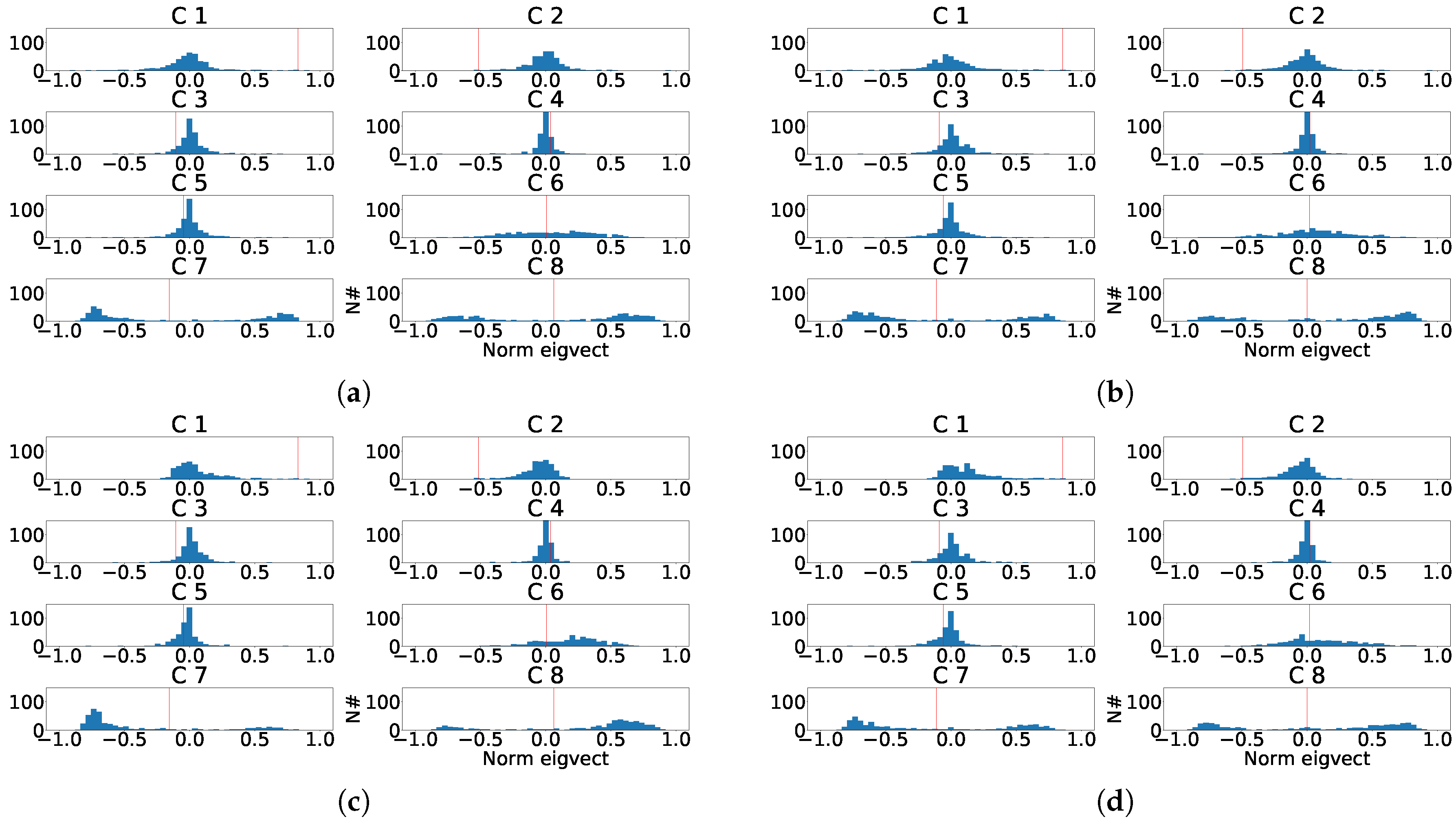
Figure 21.
Distribution of the eigenvector components values for the last principal component of the eight independent lead model. (a) Distribution of the eigenvector components for each control patient. (b) Distribution of the eigenvector components for each subrogated fragmented patient. (c) Aligned distribution of eigenvector components for each control patient. (d) Aligned distribution of eigenvector components for each subrogated fragmented patient. The red line shows the value of transformation vector used in the alignment.
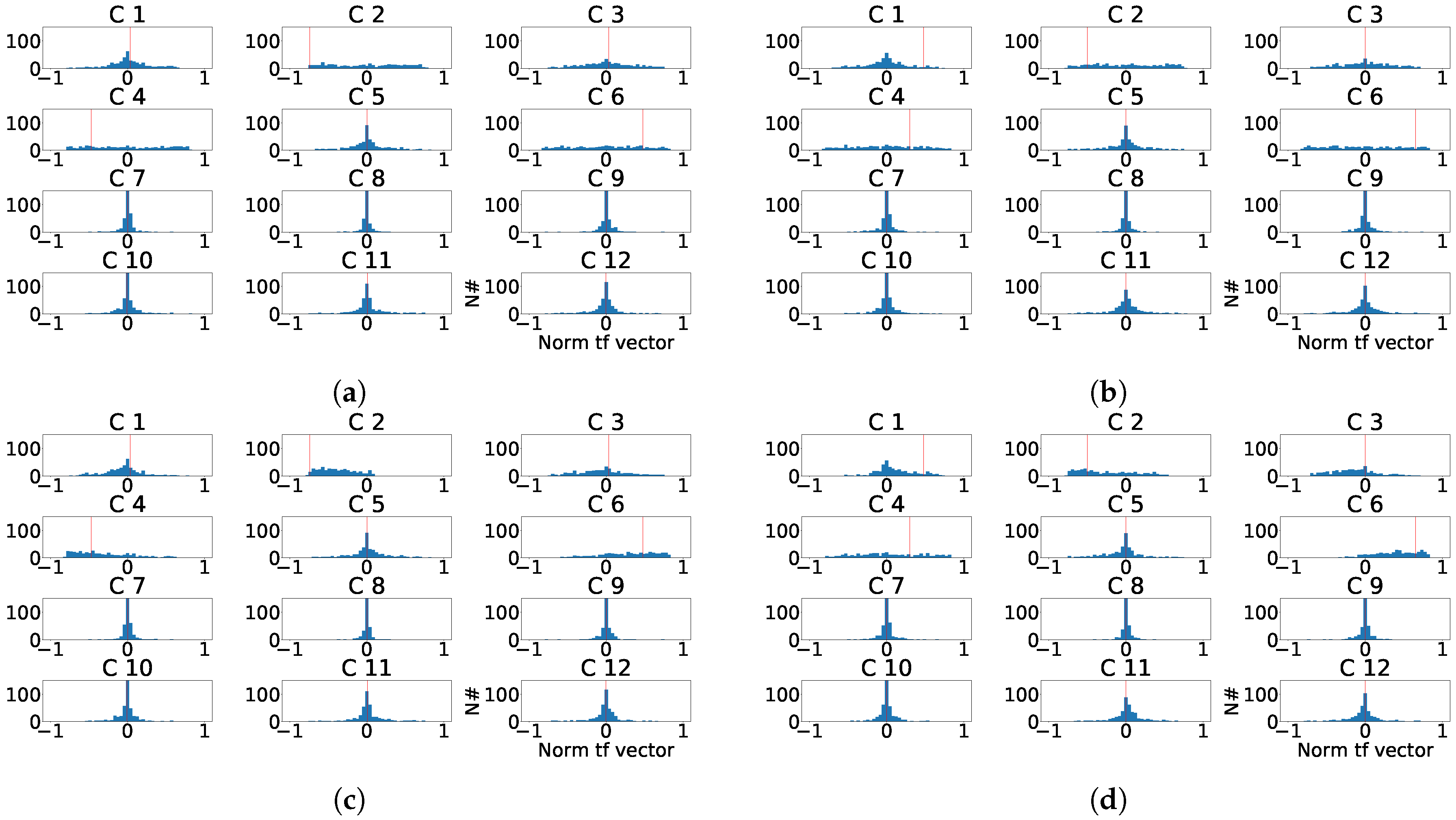
Figure 22.
Distribution of the normalized ICA transformation matrix for the last principal component of the twelve-lead model. (a) Distribution of the transformation matrix components for each control patient. (b) Distribution of the transformation matrix components for each subrogated fragmented patient. (c) Aligned distribution of transformation matrix components for each control patient. (d) Aligned distribution of transformation matrix components for each subrogated fragmented patient. The red line shows the value of transformation vector used in the alignment.
Table 1.
Normalized confusion matrix of PCA for 12-lead ECG. The value of the table represent the ratio of i-th component of control patient that is paired with the j-th component of synthetically fragmented patient according to the value of PCC.
Table 1.
Normalized confusion matrix of PCA for 12-lead ECG. The value of the table represent the ratio of i-th component of control patient that is paired with the j-th component of synthetically fragmented patient according to the value of PCC.
| | Frag 1 | Frag 2 | Frag 3 | Frag 4 | Frag 5 | Frag 6 | Frag 7 | Frag 8 | Frag 9 | Frag 10 | Frag 11 | Frag 12 |
|---|
| ctrl 1 | 1 | 0 | 0 | 0 | 0 | 0 | 0 | 0 | 0 | 0 | 0 | 0 |
| ctrl 2 | 0 | 0.998 | 0.002 | 0 | 0 | 0 | 0 | 0 | 0 | 0 | 0 | 0 |
| ctrl 3 | 0 | 0.002 | 0.986 | 0.005 | 0 | 0 | 0 | 0 | 0.002 | 0.002 | 0 | 0.002 |
| ctrl 4 | 0 | 0 | 0.012 | 0.959 | 0.012 | 0.005 | 0.002 | 0 | 0 | 0.002 | 0.005 | 0.002 |
| ctrl 5 | 0 | 0 | 0 | 0.036 | 0.906 | 0.031 | 0.002 | 0.002 | 0.002 | 0.007 | 0.007 | 0.005 |
| ctrl 6 | 0 | 0 | 0 | 0 | 0.077 | 0.834 | 0.039 | 0.029 | 0.002 | 0.002 | 0.01 | 0.007 |
| ctrl 7 | 0 | 0 | 0 | 0 | 0.005 | 0.123 | 0.773 | 0.053 | 0.019 | 0.007 | 0.012 | 0.007 |
| ctrl 8 | 0 | 0 | 0 | 0 | 0 | 0.007 | 0.176 | 0.728 | 0.048 | 0.017 | 0.017 | 0.007 |
| ctrl 9 | 0 | 0 | 0 | 0 | 0 | 0 | 0 | 0.178 | 0.713 | 0.075 | 0.024 | 0.01 |
| ctrl 10 | 0 | 0 | 0 | 0 | 0 | 0 | 0.002 | 0.005 | 0.195 | 0.728 | 0.058 | 0.012 |
| ctrl 11 | 0 | 0 | 0 | 0 | 0 | 0 | 0.005 | 0.002 | 0.007 | 0.159 | 0.781 | 0.046 |
| ctrl 12 | 0 | 0 | 0 | 0 | 0 | 0 | 0 | 0.002 | 0.01 | 0 | 0.087 | 0.901 |
Table 2.
Normalized confusion matrix of PCA for the 8 independent leads from ECG. The value of the table represent the ratio of i-th component of control patient that is paired with the j-th component of synthetically fragmented patient according to the value of PCC.
Table 2.
Normalized confusion matrix of PCA for the 8 independent leads from ECG. The value of the table represent the ratio of i-th component of control patient that is paired with the j-th component of synthetically fragmented patient according to the value of PCC.
| | Frag 1 | Frag 2 | Frag 3 | Frag 4 | Frag 5 | Frag 6 | Frag 7 | Frag 8 |
|---|
| ctrl 1 | 1 | 0 | 0 | 0 | 0 | 0 | 0 | 0 |
| ctrl 2 | 0 | 0.995 | 0.002 | 0 | 0 | 0 | 0 | 0.002 |
| ctrl 3 | 0 | 0.005 | 0.988 | 0.005 | 0 | 0.002 | 0 | 0 |
| ctrl 4 | 0 | 0 | 0.007 | 0.959 | 0.022 | 0.01 | 0 | 0.002 |
| ctrl 5 | 0 | 0 | 0.002 | 0.036 | 0.887 | 0.048 | 0.024 | 0.002 |
| ctrl 6 | 0 | 0 | 0 | 0 | 0.089 | 0.824 | 0.077 | 0.01 |
| ctrl 7 | 0 | 0 | 0 | 0 | 0 | 0.113 | 0.853 | 0.034 |
| ctrl 8 | 0 | 0 | 0 | 0 | 0.002 | 0.002 | 0.046 | 0.949 |
Table 3.
Normalized confusion matrix for each heart region, (a) antero-septal, (b) lateral region, and (c) inferior region by using PCA. For each one, the value of the table represent the ratio of i-th component of control patient that is paired with the j-th component of synthetically fragmented patient according to the value of PCC.
| (a) | (b) | (c) |
|---|
| | Frag 1 | Frag 2 | Frag 3 | Frag 4 | Frag 1 | Frag 2 | Frag 3 | Frag 4 | Frag 1 | Frag 2 | Frag 3 |
| Ctrl 1 | 1 | 0 | 0 | 0 | 1 | 0 | 0 | 0 | 1 | 0 | 0 |
| Ctrl 2 | 0 | 0.993 | 0 | 0.007 | 0 | 0.986 | 0.007 | 0.007 | 0 | 1 | 0 |
| Ctrl 3 | 0 | 0.007 | 0.986 | 0.007 | 0 | 0.014 | 0.935 | 0.051 | 0 | 0 | 1 |
| Ctrl 4 | 0 | 0 | 0.014 | 0.986 | 0 | 0 | 0.058 | 0.942 | | | |
Table 4.
Summary table with the relevant values for each proposed method based on PCA.
Table 4.
Summary table with the relevant values for each proposed method based on PCA.
| Model | Lead Number | Enhancement | Component Number |
|---|
| twelve-lead | 12 | 0.998 | 5 |
| independent-lead | 8 | 0.995 | 3 |
| Regions | 4/4/3 | 0.942/0.957/0.862 | 3/4/3 |
Table 5.
Normalized confusion matrix of ICA for the twelve-lead ECG. The value of the table represent the ratio of i-th component of control patient that is paired with the j-th component of synthetically fragmented patient according to the value of PCC.
Table 5.
Normalized confusion matrix of ICA for the twelve-lead ECG. The value of the table represent the ratio of i-th component of control patient that is paired with the j-th component of synthetically fragmented patient according to the value of PCC.
| | Frag 1 | Frag 2 | Frag 3 | Frag 4 | Frag 5 | Frag 6 | Frag 7 | Frag 8 | Frag 9 | Frag 10 | Frag 11 | Frag 12 |
|---|
| Ctrl 1 | 0.40 | 0.26 | 0.22 | 0.08 | 0.02 | 0.00 | 0.00 | 0.00 | 0.00 | 0.00 | 0.00 | 0.00 |
| Ctrl 2 | 0.19 | 0.31 | 0.23 | 0.18 | 0.06 | 0.02 | 0.01 | 0.00 | 0.00 | 0.00 | 0.00 | 0.00 |
| Ctrl 3 | 0.14 | 0.15 | 0.24 | 0.25 | 0.16 | 0.03 | 0.02 | 0.00 | 0.00 | 0.00 | 0.00 | 0.00 |
| Ctrl 4 | 0.10 | 0.11 | 0.12 | 0.26 | 0.27 | 0.11 | 0.02 | 0.00 | 0.00 | 0.00 | 0.00 | 0.00 |
| Ctrl 5 | 0.07 | 0.05 | 0.07 | 0.10 | 0.27 | 0.31 | 0.09 | 0.02 | 0.01 | 0.00 | 0.01 | 0.00 |
| Ctrl 6 | 0.04 | 0.04 | 0.04 | 0.05 | 0.07 | 0.31 | 0.37 | 0.05 | 0.01 | 0.01 | 0.00 | 0.00 |
| Ctrl 7 | 0.01 | 0.03 | 0.02 | 0.03 | 0.06 | 0.11 | 0 | 0.32 | 0.06 | 0.01 | 0.00 | 0.01 |
| Ctrl 8 | 0.01 | 0.01 | 0.01 | 0.02 | 0.03 | 0.04 | 0.07 | 0.42 | 0.32 | 0.05 | 0.01 | 0.01 |
| Ctrl 9 | 0.00 | 0.01 | 0.01 | 0.01 | 0.01 | 0.02 | 0.02 | 0.08 | 0.44 | 0.33 | 0.06 | 0.00 |
| Ctrl 10 | 0.01 | 0.00 | 0.01 | 0.01 | 0.02 | 0.01 | 0.02 | 0.03 | 0.07 | 0.48 | 0.27 | 0.07 |
| Ctrl 11 | 0.01 | 0.01 | 0.01 | 0.01 | 0.02 | 0.01 | 0.01 | 0.03 | 0.05 | 0.08 | 0.53 | 0.22 |
| Ctrl 12 | 0.01 | 0.02 | 0.02 | 0.01 | 0.01 | 0.02 | 0.03 | 0.04 | 0.03 | 0.03 | 0.11 | 0.67 |
Table 6.
Normalized confusion matrix for each heart region for ICA model, for (a) antero-septal, (b) lateral region, and (c) inferior region using ICA plus kurtosis. For each one, the value of the table represents the ratio of i-th component of control patient that is paired with the j-th component of synthetically fragmented patient according to the value of PCC.
| (a) | (b) | (c) |
|---|
| | Frag 1 | Frag 2 | Frag 3 | Frag 4 | Frag 1 | Frag 2 | Frag 3 | Frag 4 | Frag 1 | Frag 2 | Frag 3 |
| Ctrl 1 | 0.73 | 0.22 | 0.06 | 0.00 | 0.78 | 0.19 | 0.03 | 0.00 | 0.67 | 0.30 | 0.02 |
| Ctrl 2 | 0.18 | 0.66 | 0.17 | 0.00 | 0.15 | 0.67 | 0.16 | 0.01 | 0.30 | 0.64 | 0.06 |
| Ctrl 3 | 0.08 | 0.12 | 0.76 | 0.04 | 0.05 | 0.14 | 0.76 | 0.05 | 0.02 | 0.06 | 0.92 |
| Ctrl 4 | 0.01 | 0.01 | 0.02 | 0.96 | 0.01 | 0.00 | 0.05 | 0.94 | | | |
Table 7.
Normalized confusion matrix of ICA over 8 independent lead model. The value of the table represent the ratio of i-th component of control patient that is paired with the j-th component of synthetically fragmented patient according to the value of PCC.
Table 7.
Normalized confusion matrix of ICA over 8 independent lead model. The value of the table represent the ratio of i-th component of control patient that is paired with the j-th component of synthetically fragmented patient according to the value of PCC.
| | Frag 1 | Frag 2 | Frag 3 | Frag 4 | Frag 5 | Frag 6 | Frag 7 | Frag 8 |
|---|
| Ctrl 1 | 0.59 | 0.26 | 0.12 | 0.02 | 0.01 | 0.00 | 0.00 | 0.00 |
| Ctrl 2 | 0.18 | 0.46 | 0.24 | 0.11 | 0.01 | 0.01 | 0.00 | 0.00 |
| Ctrl 3 | 0.10 | 0.11 | 0.46 | 0.25 | 0.07 | 0.01 | 0.00 | 0.01 |
| Ctrl 4 | 0.05 | 0.05 | 0.07 | 0.46 | 0.30 | 0.05 | 0.01 | 0.01 |
| Ctrl 5 | 0.03 | 0.03 | 0.04 | 0.07 | 0.51 | 0.26 | 0.05 | 0.02 |
| Ctrl 6 | 0.02 | 0.02 | 0.01 | 0.04 | 0.05 | 0.54 | 0.28 | 0.04 |
| Ctrl 7 | 0.01 | 0.03 | 0.02 | 0.02 | 0.02 | 0.07 | 0.59 | 0.23 |
| Ctrl 8 | 0.02 | 0.04 | 0.03 | 0.03 | 0.04 | 0.07 | 0.08 | 0.69 |
Table 8.
Summary table with the most relevant values of each proposed method based on ICA.
Table 8.
Summary table with the most relevant values of each proposed method based on ICA.
| Model | Lead Number | Enhancement | Component Number |
|---|
| twelve-lead | 12 | 99.52 | 4 |
| independent leads | 8 | 98.4 | 4 |
| Regions | 4/4/3 | 92.08/92.03/87.68 | 4/4/3 |

