An Improved Second-Order Blind Identification (SOBI) Signal De-Noising Method for Dynamic Deflection Measurements of Bridges Using Ground-Based Synthetic Aperture Radar (GBSAR)

Abstract

Ground-based synthetic aperture radar (GBSAR) technology has been widely used for bridge dynamic deflection measurements due to its advantages of non-contact measurements, high frequency, and high accuracy. To reduce the influence of noise in dynamic deflection measurements of bridges using GBSAR—especially for noise of the instantaneous vibrations of the instrument itself caused by passing vehicles—an improved second-order blind identification (SOBI) signal de-noising method is proposed to obtain the de-noised time-series displacement of bridges. First, the obtained time-series displacements of three adjacent monitoring points in the same time domain are selected as observation signals, and the second-order correlations among the three time-series displacements are removed using a whitening process. Second, a mixing matrix is calculated using the joint approximation diagonalization technique for covariance matrices and to further obtain three separate signal components. Finally, the three separate signal components are converted in the frequency domain using the fast Fourier transform (FFT) algorithm, and the noise signal components are identified using a spectrum analysis. A new, independent, separated signal component matrix is generated using a zeroing process for the noise signal components. This process is inversely reconstructed using a mixing matrix to recover the original amplitude of the de-noised time-series displacement of the middle monitoring point among three adjacent monitoring points. The results of both simulated and on-site experiments show that the improved SOBI method has a powerful signal de-noising ability.

1. Introduction

With the rapid deployment of transportation networks, an increased number of bridges have been built in the world. However, a combination of factors such as age, environment, overload, and geological activities have increased the deterioration of bridges, which can ultimately lead to a reduction in their load carrying capacity—or even sudden collapse—leading to a loss of life and property [1,2]. Therefore, damage detection for bridges is of the utmost importance. Ground-based synthetic aperture radar (GBSAR) technology is a new type of ground-based microwave interferometry technology with the advantages of real-time monitoring, high-distance resolution, fast measurement speed, high precision, wide measurement coverage, easy operation, and all-weather and all-day measurements [3,4]. Since the first published paper (in 1999) on microwave interferometry for non-contact vibration measurements on large structures [5], GBSAR has been used extensively for dynamic deflection measurements of bridges in recent years [6,7]. However, during the data acquisition process of dynamic deflection measurements of bridges using GBSAR, the surrounding environment, human operation, and the equipment itself will inevitably increase noise in the obtained time-series displacements, which reduces the damage detection accuracy [8]. In particular, the used GBSAR equipment should be placed under the monitored bridge, and the instantaneous vibrations of the equipment itself will be inevitably caused by passing vehicles under the monitored bridge, which will reduce the accuracy of the obtained dynamic time-series displacement. Therefore, it is of great importance to reduce the influence of noise information in the time-series displacements of bridges obtained using GBSAR—especially for the instantaneous vibrations of the equipment itself.

Currently, the primary signal de-noising methods for the time-series data include the filtering method [9,10,11,12], the wavelet transform method [13,14], the singular value decomposition method [15,16], and the empirical mode decomposition (EMD) method [17,18,19]. Filtering methods use statistical features to derive some estimation algorithms, and further estimate the useful signals or filter the signals with certain statistical features from the mixed signal, which can improve the signal-to-noise ratio (SNR). However, they remove not only noise, but also the high frequency components of non-stationary signals, and normally require a priori information of the statistical characteristics of the signal and noise, which are not effective for non-stationary signals containing sharp edges and impulses of short duration [9,10,12]. Therefore, without any priori information of the obtained dynamic time-series displacement, filtering methods are not suitable for signal de-nosing of the non-stationary dynamic time-series displacement obtained using GBSAR. With the advantage of a good time-frequency localization characteristic, the wavelet transform can be used to obtain the wavelet coefficients of signal and noise with different properties on each scale. This method can further remove the wavelet coefficient of the noise portion to obtain the de-noised signal by reconstructing the remaining wavelet coefficients, which is suitable for analyzing non-stationary signals [13]. However, there are two main limitations of the wavelet transform: first of, the results are affected by the selection of the wavelet basis, and different noise frequency scales need different wavelet threshold criteria, which cause a lack of adaptability [15]; secondly, it is not suitable for non-linear signals [17]. In this study, the obtained time-series displacement should be a non-linear signal in case the monitored bridge was damaged. Moreover, it is also difficult to determine the suitable wavelet basis and wavelet threshold criteria as the instantaneous vibrations of the equipment itself caused by passing vehicles with different speed and weight. The singular value decomposition method primarily depends on the correspondence between the information of the signal and the singular value of the reconstruction matrix. The signal component corresponding to the noise is a smaller singular value. By retaining the larger singular values first, the optimal approximation of the original signal can be obtained, and the influence of the noise can be eliminated [15]. However, there are two critical issues to be solved: the first issue is how to determine the effective rank order of the reconstruction matrix, and the second issue is how to determine the number of rows and columns in the reconstruction matrix—which restricts the applications of this method [16]. Recently, the EMD method was introduced for analyzing signals from nonlinear, nonstationary processes, which can adaptively decompose the non-stationary signal into a series of intrinsic mode functions (IMFs), and the decomposed into components containing local characteristic signals of different time scales of the source signal [17]. The EMD de-noising method reduces the influence of noise by eliminating a certain number of low-order IMFs with relatively high frequencies [18]. However, the IMFs decomposed using the EMD method have a mode mixing problem that causes the decomposed IMFs to contain useful components and noise—especially under dynamic conditions. This may cause a loss of precision when using the EMD de-noising method [19]. The ensemble empirical mode decomposition (EEMD) method is an improvement based on the EMD method and uses the EMD method as its core, inheriting the advantages of the EMD method [20]. The EEMD method repeatedly decomposes the original signal with added white noise into a series of IMFs and further calculates the ensemble of IMFs to alleviate mode mixing, which has been widely used in the field of signal de-noising [21,22]. However, the EEMD method is affected by parameters such as the amplitude of added noise and the number of ensemble trials [23]. Moreover, although the EMD and EEMD methods can effectively reduce the influence of the periodic noise [22], it is difficult to reduce the influence of the instantaneous noise, such as the instantaneous vibrations of the equipment itself caused by passing vehicles with a different speed and weight in this study.

Unlike the above signal de-noising methods used to reduce the influence of noise from single time-series data individually, the blind source separation (BSS) technique can separate multiple source signals acquired in the same time domain by multiple sensors without any prior information—even when the mixed model of different signals is unknown [24]. BSS has been successfully applied in the fields of wireless communication, image processing, speech signal processing, and biomedical signal processing [25]. The second-order blind identification (SOBI) method is a relatively robust blind source separation method that uses second-order statistics of the sample data (correlation matrix with different time delays) and the source signal time sequence structure feature to achieve blind separation of the source signals [26]. In recent years, the SOBI method has successfully been applied in the fields of signal processing and mechanical fault detection [27,28]. In this study, we used a new type of ground-based microwave interferometry technology, which uses multi-set time-series displacements of monitored targets in bridges in the same time domain with a distance resolution of up to 0.5 m, using GBSAR. The obtained time-series displacements of the adjacent monitoring points have the same noise information, especially for the noise of the instantaneous vibrations of the equipment itself caused by passing vehicles with a different speed and weight. Generally, the obtained dynamic deflection signal of bridges using GBSAR is a complicated non-stationary time-series displacement that mixes the useful signal with noise. Therefore, in this study, the obtained time-series displacement of three adjacent monitoring points can be regarded as a linear mixture of source signals of useful signals and noise signals. An improved SOBI signal de-noising method is proposed to reduce the influence of noise for the obtained time-series displacement using GBSAR, especially for the noise of the instantaneous vibrations of the equipment itself caused by passing vehicles with different speed and weight.

2. Methodology

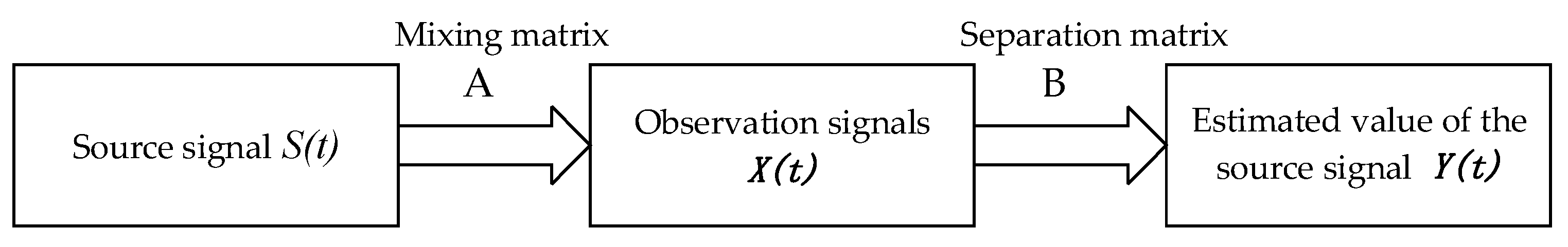
2.1. BSS Model

The SOBI method is a relatively robust BSS algorithm that can be used to decompose mixtures of signals into a set of components or putative recovered sources [29]. To better understand the improved SOBI method, the principle of BSS is introduced first. Figure 1 shows an instantaneous linear BSS system model. $S\left(t\right)={[s_1\left(t\right)s_2\left(t\right)\dots s_n(t)]}^T$ represents $n$ statistically independent unknown source signals. $X\left(t\right)={[x_1\left(t\right)x_2\left(t\right)\dots x_m(t)]}^T$ denotes $m$ observation signals. Then, let $X\left(t\right)=A*S\left(t\right)$, where $A$ denotes a mixing matrix of $m*n$ dimensions [29,30]. The essence of BSS is to find a separation matrix $B$, so that $Y(t)=BX(t)$ is an optimal estimate of the source signal, which is obtained from the original observation signal $X\left(t\right)$ through the separation matrix $B$.

In this study, the prior information of the source signals (time-series displacements without noise) and the mixing matrix were unknown—only the observed signals (time-series displacement obtained using GBSAR) were processed to obtain the different source signals. However, in the absence of any underlying assumptions and more information, multiple solutions will be produced by BSS. Therefore, it is necessary to make some underlying assumptions and conditions to constrain the source signal and the mixing matrix, and then solve the problem of the multiple solutions. The underlying assumptions and conditions are described as follows [26,30]:

(1)

Mixing matrix, A, is a column full-rank matrix.

(2)

The source signals are the zero-mean random signals that are not correlated in the time-space domain and correlated in the time domain.

(3)

The source signal and noise are independent.

(4)

The number of source signals is less than or equal to the number of the original signals.

Moreover, when both the mixing matrix, $A$, and the source signal, $S\left(t\right)$, are unknown, each column of $A$ and the corresponding row of $S\left(t\right)$ are multiplied by a factor that is reciprocal to each other. In addition, $X\left(t\right)$ is unchanged, which is shown as follows:

$$X\left(t\right)=A*S\left(t\right)={\displaystyle \sum _{i=1}^M{a}_i{s}_i(t)}={\displaystyle \sum _{i=1}^M(a_i/b_i)(b_i{s}_i(t)}),$$

(1)

where $b_i\ne 0$ is an arbitrary constant. In the case where $A$ is unknown, as shown in Equation (1), it cannot be determined whether the source signal is $s_i(t)$ or $b_i{s}_i(t)$—that is, the amplitude of the source signal cannot be determined. Therefore, even if the above underlying assumptions and constraints are applied to the obtained time-series displacement, there are still two uncertainties in BSS—that is, the amplitude and component sequence of the separated source signals are uncertain [29,31,32]. However, the separated signal is consistent with the waveform of the source signal. In this study, the uncertainty of the component sequence does not affect the result, and the uncertainty of the amplitude of the separated signals are restored using the improved SOBI algorithm.

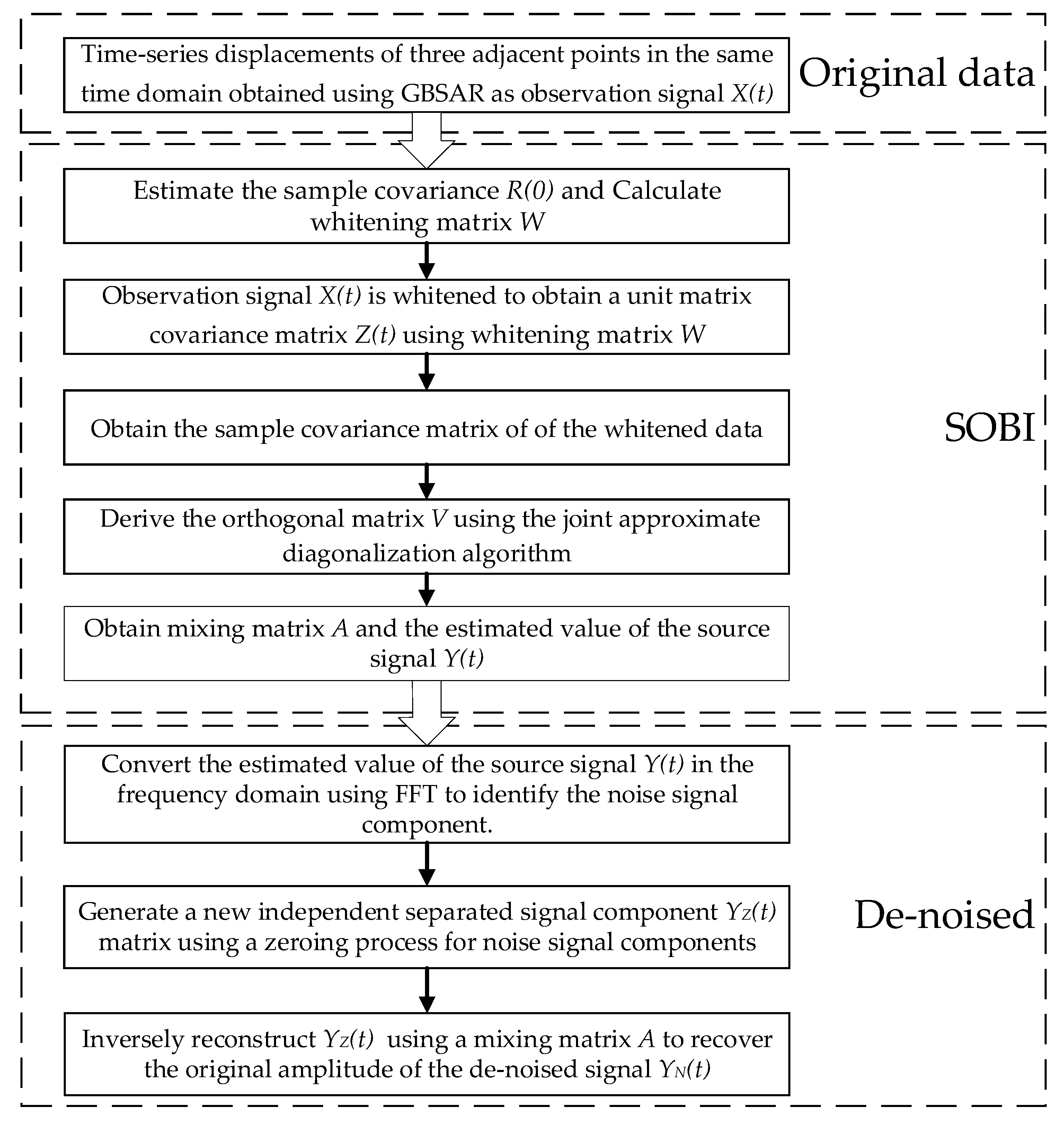
2.2. Improved SOBI

The SOBI method uses joint approximation diagonalization to process the covariance matrix, which can solve the best estimation of the source signal and the mixing matrix and further obtain the separated signal components from different source signals. It is a relatively robust blind source separation method [26]. The SOBI method is based on the second-order statistics of the original observation data, which can estimate the source signal component and separate multiple Gaussian noise sources using relatively few data points [33]. By considering the linear mixed model together with the characteristics of the obtained time-series displacement using GBSAR, it is proposed in this study to select the obtained time-series displacements of three adjacent monitoring points in the same time domain as the original signals to obtain the de-noised signal of the middle point among the three adjacent monitoring points. The three time-series displacements can be regarded as a linear mixture of source signals of useful information and noise.

The basic principle of the improved SOBI signal de-nosing method is based on a time correlation of the source signal and the joint approximation diagonalization of the covariance matrix [27]. When it is applied to signal de-noising, the noise information is separated and zeroed by the other two sets of data, and the mixed matrix is used to inversely reconstruct the signal to obtain the de-noised signal. Figure 2 shows the entire workflow of the improved SOBI signal de-noising method for the obtained time-series displacement of bridges using GBSAR. The workflow includes the following four key technologies: (1) the observation signal, $X\left(t\right)$, is whitened to obtain a unit matrix covariance matrix, $Z\left(t\right)$. The second-order correlation among the signal components is removed, and the sampling covariance matrix of the whitened data, $Z\left(t\right)$, is calculated. (2) The orthogonal matrix is obtained using joint approximate diagonalization of the covariance matrix with different time delays. (3) The estimated value of the source signal, $Y\left(t\right)$, and the mixing matrix, $A$, are calculated using the orthogonal matrix. (4) The estimated value of the source signal, $Y\left(t\right)$, is converted in the frequency domain using the fast Fourier transform (FFT), and the noise signal component is identified using the frequency characteristics. A new independent separated signal component matrix, $Y_Z\left(t\right)$, is generated using a zeroing process for noise signal components, which is inversely reconstructed using a mixing matrix, $A$, to recover the original amplitude of the de-noised signal, $Y_N\left(t\right)$.

Denote $X\left(t\right)={[x_1\left(t\right)x_2\left(t\right)x_3(t)]}^T$ as mixed signals of time-series displacements of three adjacent points in the same time domain, and denote $S\left(t\right)={[s_1\left(t\right)s_2\left(t\right)s_3(t)]}^T$ as the source signals, which are assumed to be independent of each other. In addition, denote $Y\left(t\right)$ as the estimated value of the source signal. The detailed steps of the improved SOBI de-noising method for the obtained time-series displacement of bridges using GBSAR are as follows [26,28,34]:

(1) Estimate the sample covariance, $R(0)$, from the three sets of original observation signals (time-series displacements of three adjacent monitoring points), denote ${\lambda }_1,{\lambda }_2,{\lambda }_3$ as the largest eigenvalues and $h_1,h_2,h_3$ as the corresponding eigenvectors of $R(0)$.

(2) In the case where white noise is assumed to exist, the estimated value of the noise variance, ${\sigma }^2$, is the average of the smallest eigenvalues of $R(0)$. The whitening signal is $Z\left(t\right)={[z_1\left(t\right)z_2\left(t\right)z_3(t)]}^T$, where $z_i\left(t\right)={({\lambda }_i-{\sigma }^2)}^{-\frac{1}{2}}{h}_i*x(t)$, $(i=1,2,3)$. This is equivalent to forming a whitening matrix as follows:

$$W={[{({\lambda }_1-{\sigma }^2)}^{-\frac{1}{2}}{h}_1,\dots ,{({\lambda }_3-{\sigma }^2)}^{-\frac{1}{2}}{h}_3]}^T.$$

(2)

(3) Denote $W$ as a whitening matrix, and the original observation signals, $X\left(t\right)$, are whitened to remove the second-order correlation between the signal components to obtain a unit covariance matrix, $Z(t)$:

$$Z(t)=W*X\left(t\right)=W*A*S\left(t\right)=V*S\left(t\right).$$

(3)

(4) For fixed time lags, $\tau \in \left\{{\tau }_j\right|j=1,2,\mathrm{..}k\}$, the sample covariance matrix, $R\left(\tau \right)$, of the whitened data is calculated using $R\left(\tau \right)=E\left[Z\left(t\right)Z^T\left(t+\tau \right)\right]=A{R}_Z\left(\tau \right)A^T$.

(5) For all $R\left({\tau }_j\right)$, the joint approximate diagonalization algorithm is used to derive the orthogonal matrix, $V$.

(6) The estimated value of the source signal is obtained using $Y(t)=BX(t)=V^{T}WX(t)$, and the mixing matrix, $A$, is estimated as $A=W^{-1}V$, where $W^{-1}$ is the pseudo inverse matrix of the whitening matrix, $W$.

(7) The fast Fourier transform (FFT) algorithm is used to perform a spectral conversion on the separated signal components to find the noise signal components for the zeroing processing combined with a frequency analysis. The estimated value of the mixing matrix, $A$, is used for the reverse reconstruction:

$$Y_N\left(t\right)=A*Y_Z\left(t\right),$$

(4)

where $Y_N\left(t\right)$ is the reconstructed signal component as the de-noised signal; $A$ is the estimation of the mixing matrix; and $Y_Z\left(t\right)$ is a source signal matrix obtained by zeroing the unwanted noise signal components in the estimated value of the source signal, $Y\left(t\right)$.

2.3. Accuracy Assessment

To evaluate the signal de-noising quality of the improved SOBI signal de-noising method, four objective evaluation indexes were used in this study. These include the noise rejection ratio (NRR) [35], the noise mode (NM) [36,37], the signal energy ratio (SER) [36,37], and the root mean square error (RMSE) [35].

NRR can reflect the ability to suppress interference and improve SNR. NRR is defined as:

$$NRR=10(\lg {\delta }_1{}^2-\lg {\delta }_2{}^2),$$

(5)

where ${\delta }_1$ and ${\delta }_2$ are the quasi-deviations of the signals before and after signal de-noising, respectively.

SER and NM are the quantitative evaluations of noise removal efficiency and noise quantity from the energy point of view, respectively. SER reflects the energy similarity between the de-noised signal and the original signal, and NM reflects the overall level of noise. The SER and NM are defined as:

$$SER=\sqrt{{\displaystyle \sum _{n=1}^N{y}^2(n)}}/\sqrt{{\displaystyle \sum _{n=1}^N{s}^2(n)}},$$

(6)

$$NM=\sqrt{{\displaystyle \sum _{n=1}^N{(y(n)-s(n))}^2}},$$

(7)

where $s(n)$ represents the original observation signal; $y(n)$ represents the signal after noise reduction; and $n$ represents the number of sampling points.

RMSE is used to measure the deviation between the observed value and the true value. The RMSE is defined as:

$$RMSE=\sqrt{\frac{1}{N}{\displaystyle \sum _{n=1}^N{(y(n)-s(n))}^2}},$$

(8)

where $s(n)$ represents the original observation signal; $y(n)$ represents the signal after noise reduction; and $n$ represents the number of sampling points.

Generally, the larger the NRR and NM values are, the closer the NM value is to one. Additionally, the smaller the RMSE value is, the more enhanced the signal de-noising is.

3. Simulated Experiment and Analysis

To validate the ability of the improved SOBI signal de-noising method to distinguish the useful signal and noise, a simulation example was conducted in this study. The application of the time-series displacements of three adjacent monitoring points used to obtain the de-noised time-series displacement of the middle monitoring point among three adjacent monitoring points, can be regarded as a linear mixture of source signals of useful signal and noise signal. Therefore, three simulated sub-signals, which included two useful sub-signals, were constructed; $s_1(t)$ (Figure 3a) and $s_2(t)$ (Figure 3b), and a noise signal, $s_3(t)$ (Figure 3c), of which the waveforms are shown in Figure 3.

$$s_1(t)=0.3sin(3\pi t),$$

(9)

$$s_2(t)=(0.2+0.3sin(4\pi t))+0.5cos(2\pi t)+cos(10\pi t),$$

(10)

$$s_3(t)=0.1randn\left(1,N\right),$$

(11)

where the sampling point $N$ is 600 for the noise signal $S_3(t)$, and the sampling frequency is 200 HZ. Moreover, the mixing matrix $A$ is a random matrix, which meets the requirement of a column full rank matrix. In this study, the mixing matrix $A$ is defined as follows:

$$A=\left[\begin{array}{ccc}0.2& 0.7& 0.5\\ 0.4& 0.3& 0.4\\ 0.1& 0.9& 0.8\end{array}\right].$$

(12)

As shown in Figure 4, the three mixed signals were linearly mixed using three sets of simulation source signals. Each mixed signal contained the characteristic information of the three sets of source signals. Without more prior information, the characteristic information of the source signals could not be obtained intuitively from the mixed signals. Using the improved SOBI method, three sets of signals were separated from the three mixed signals.

As shown in Figure 5, the three separated sub-signals are consistent with the three source signals in the waveform characteristics. To further evaluate the accuracy of the separated results, correlation coefficients between the separated signal and the source signal were calculated using Equation (13):

$$C={\displaystyle \sum _{n=1}^N(Y_n(t)-{\overline{Y}}_n(t))(S_n(t)-{\overline{S}}_n(t))}/\sqrt{{\displaystyle \sum _{n=1}^N{(Y_n(t)-{\overline{Y}}_n(t))}^2*{\displaystyle \sum _{n=1}^N{(S_n(t)-{\overline{S}}_n(t))}^2}}},$$

(13)

where $S_n(t)$ is the source signal, ${\overline{S}}_n(t)$ represents the average value of the source signal, $Y_n(t)$ is the separated signal, and ${\overline{Y}}_n(t)$ represents the average of the separated signals.

As shown in

Table 1. Correlation coefficient between the separated signal and the source signal.

Signal Components	Correlation Coefficients
	${\mathit{S}}_1(\mathit{t})$	${\mathit{S}}_2(\mathit{t})$	${\mathit{S}}_3(\mathit{t})$
$Y_1(t)$	0.9933	−0.0173	0.0555
$Y_2(t)$	0.1155	0.9999	−0.0133
$Y_3(t)$	−0.0016	0.0003	0.9984

, the correlation coefficients between each simulated source signal and the corresponding separated signal component are all greater than 0.99, which indicates that the improved SOBI method effectively separated different source signals from the mixed signals. In particular, for the noise source signal and the corresponding separated signal component, the correlation coefficient is 0.9984, which can effectively distinguish the useful and noise signal and further perform signal de-noising. In this study, for the obtained time-series displacements using GBSAR, the useful and noise signals were regarded as independent source signals. Therefore, the noise in the obtained time-series displacements was effectively reduced using the improved SOBI signal de-noising method.

4. On-Site Experiment and Analysis

4.1. Site Description and Data Acquisition

The Fengbei Bridge is located at the junction of the West Fourth Ring Road and the Fengtai North Road in Beijing, China. As shown in Figure 6a, there is a road crossing under the bridge, and the GB-SAR instrument should be located on one side of the bridge as shown in Figure 6b. Inevitably, the different instantaneous vibrations of the equipment itself will be caused by passing vehicles with a different speed and weight on the road, which increases the noise in the obtained time-series displacement of the bridge. Therefore, to validate the accuracy of the improved SOBI signal de-noising method for time-series displacement obtained using GBSAR, the Fengbei Bridge was selected as an experimental bridge. In this study, an Imaging by Interferometric Survey (IBIS-S) instrument—a typical system based on microwave interferometry—was adopted to acquire an accurate dynamic time-series displacement of the bridge dynamic deflection. The IBIS-S instrument consists of a radar unit, a control personal computer, a power supply unit, and a tripod. In typical measurement conditions, the sampling rate is up to 200 Hz, the maximal detection distance is up to 1 km, the range resolution is up to 0.50 m, and the displacement measurement accuracy is up to 0.01 mm [38]. As shown in Figure 6, the IBIS-S instrument was located on one side of the bridge without passive radar reflectors attached to the bridge. The angle of the altitude of the radar unit was set to 30° so that the two antennas on the radar unit could be aligned to the mid-span point of the central span of the bridge. The range resolution was 0.5 m, the sampling frequency was 200 Hz, and the duration of data acquisition was 45 s.

Figure 7a shows the obtained time-series displacement (X1, as shown in Figure 6a) of a mid-span point on the Fengbei Bridge. Due to the influences of the surrounding environment and the equipment itself, there was an inevitable increase in the noise information of the obtained time-series displacement. Therefore, to improve the accuracy of the obtained time-series displacement of the mid-span point on the Fengbei Bridge, using a similar noise as the time-series displacements from the mid-span point, two adjacent monitored points before and after the mid-span point were selected as another two observed signal point (X2 and X3, as shown in Figure 6a). This was done to develop signal de-noising for the mid-span point of the Fengbei Bridge using the improved SOBI method. The time-series displacements of the two adjacent monitored points are shown in Figure 7b,c. Obviously, there are some fluctuations in the curves of the obtained three time-series displacements. These were caused by the transient load of vehicles.

4.2. Results Analysis and Discussion

Three separate signal components were obtained using the improved SOBI signal de-noising method, namely S1, S2, and S3, as shown in Figure 8. The inspection of curves of the separated signal components shown in this figure clearly highlight that: (1) as shown in Figure 8a, the separated signal, S1, with an inverted displacement is consistent with the original time-series displacement, X1, of the mid-span point of the Fengbei Bridge, which can be regarded as actual monitored data, and; (2) as shown in Figure 8b,c, there are some sudden changes in these two curves of the separate S2 and S3 signals, which can be regarded as noise signals. These may have been caused by the passing vehicles near the IBIS-S instrument, which led to several vibrations of the IBIS-S instrument. Moreover, there are some smaller fluctuations in these two curves, which may have been caused by the surrounding environment, such as wind thrusts and ground motions. Moreover, as shown in Figure 9, the spectra of the three observed signals are basically the same, with a similar first order frequency of 2.46 Hz. In the spectrum of the separated signal, S1, found using the improved SOBI method, the first order frequency is the same as that of the three observed signals as shown in Figure 10a. This indicates that the separated signal, S1, is the useful signal. However, for the spectra of the separated signals—S2 and S3—found using the improved SOBI method, the frequencies are disorderly and irregular as shown in Figure 10b,c. This indicates that the separated signals—S2 and S3—are noise signals.

By zero processing the separated noise signal, the de-noised time-series displacement of the mid-span point was obtained by inversely reconstructing the separated signal using a mixing matrix, as shown in Figure 11. The red curve is the original signal of the obtained time-series displacement of the mid-span point, and the blue curve is the de-noised signal. Compared with the original time-series displacement, the de-noised time-series displacement is more stable and smooth. Moreover, as the six black boxes show in Figure 11, there are greater changes between the original signal and the de-noised signal. Furthermore, these six time ranges are the same as the time ranges of the sudden changes in the curves of the separated signals—S2 and S3—as shown in Figure 8b,c. The results show that the noise information caused by the passing vehicles near the IBIS-S instrument was effectively eliminated.

To validate the accuracy of the improved SOBI signal de-noising method for dynamic deflection measurements using GBSAR, two de-noising methods—EMD [20] and EEMD [22]—were selected to be compared with the improved SOBI signal de-noising method. The comparison results are shown in

Table 2. Comparison of the four evaluation indexes among the three de-noised methods.

Index	EMD	EEMD	SOBI
NRR (db)	−2.3393	3.2862	6.7116
NM (mm)	2.5066	0.7211	3.7622
SER	0.9870	0.9947	1.0012
RMSE (mm)	0.0264	0.0073	0.0120

. The inspection from this table highlights that: (1) The NRR and NM are 6.7116 db and 3.7622 mm for the improved SOBI signal de-noising method, which are much better than that of the EMD and EEMD methods. Moreover, the SER is 1.0012 for the improved SOBI signal de-noising method, which is closer to one than the other two methods. Therefore, according to these three indexes, the improved SOBI signal de-noising method had a more powerful ability than the EMD and EEMD methods for dynamic deflection measurements using GBSAR. (2) The RMSE is 0.012 mm for the improved SOBI signal de-noising method, which is smaller than that of the EMD method and greater than that of the EEMD method. The reason is that the removal of noise caused by passing vehicles near the IBIS-S instrument may have caused a reduction in the RMSE using the improved SOBI signal de-noising method. Although a smaller RMSE can be obtained using the proposed signal de-noising method if the on-site experiment was done without passing vehicles near the IBIS-S instrument, it is difficult to find a suitable time range to acquire dynamic time-series displacement data of bridges. The results indicate that the improved SOBI signal de-noising method had a powerful de-noising ability, which not only reduced the noise caused by the surrounding environment, but also reduced the noise caused by vibrations of the monitoring instrument.

5. Conclusions

Due to the advantage of the high-distance resolution of the GBSAR technique, the obtained time-series displacements of the adjacent monitoring points had a similar noise. Therefore, in this study, to improve the accuracy of the obtained dynamic time-series displacement of bridges using GBSAR, an improved SOBI signal de-nosing method was proposed to reduce the influence of noise. This was achieved by using the obtained dynamic time-series displacements of three adjacent monitoring points in the same time domain. In addition, the de-noised signal of the middle point among the three adjacent monitoring points was obtained. This was done to address the noise caused by instantaneous vibrations of the equipment itself and noise caused by passing vehicles. More specifically, the results presented in the study clearly highlight the following:

(1)

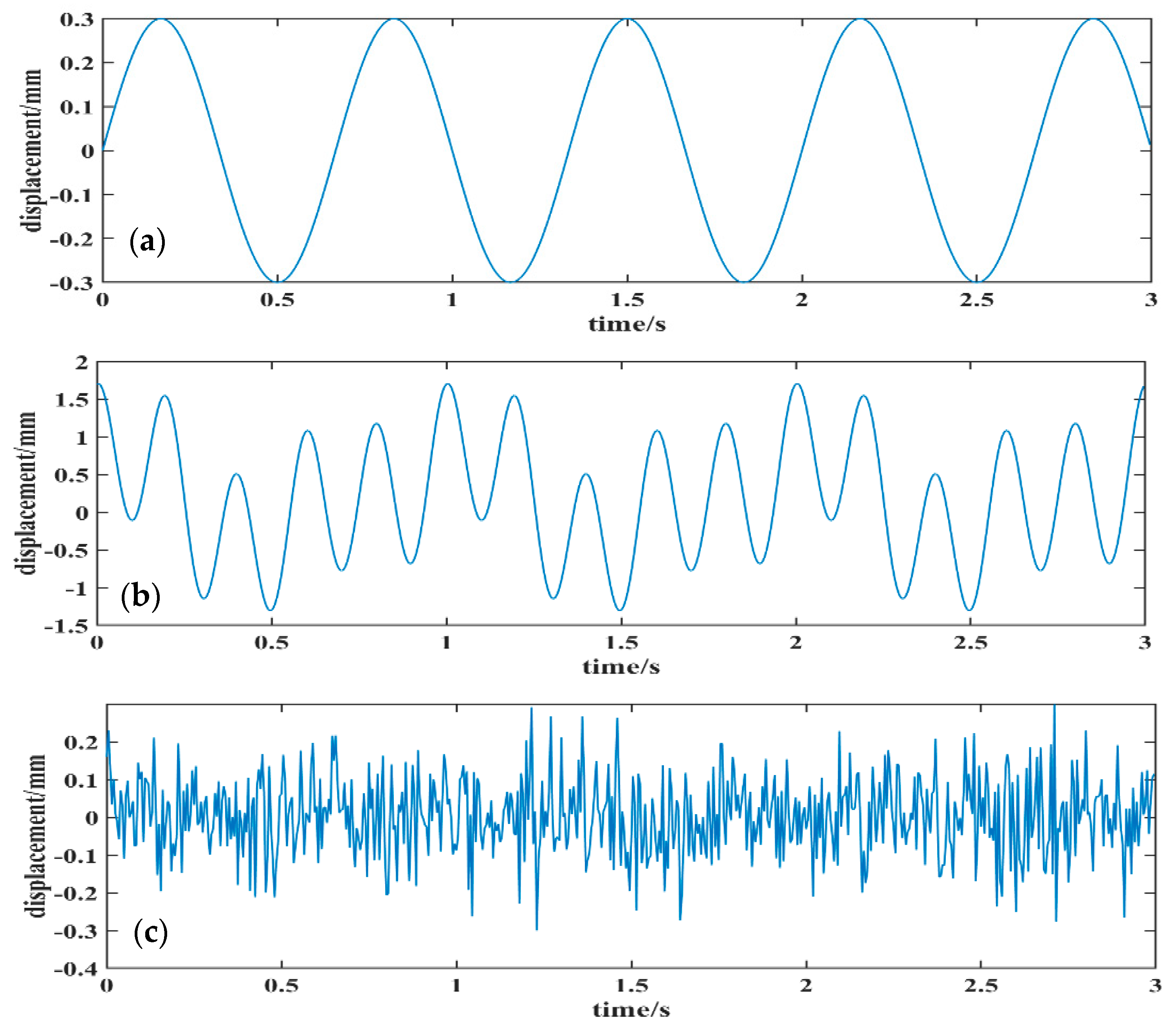
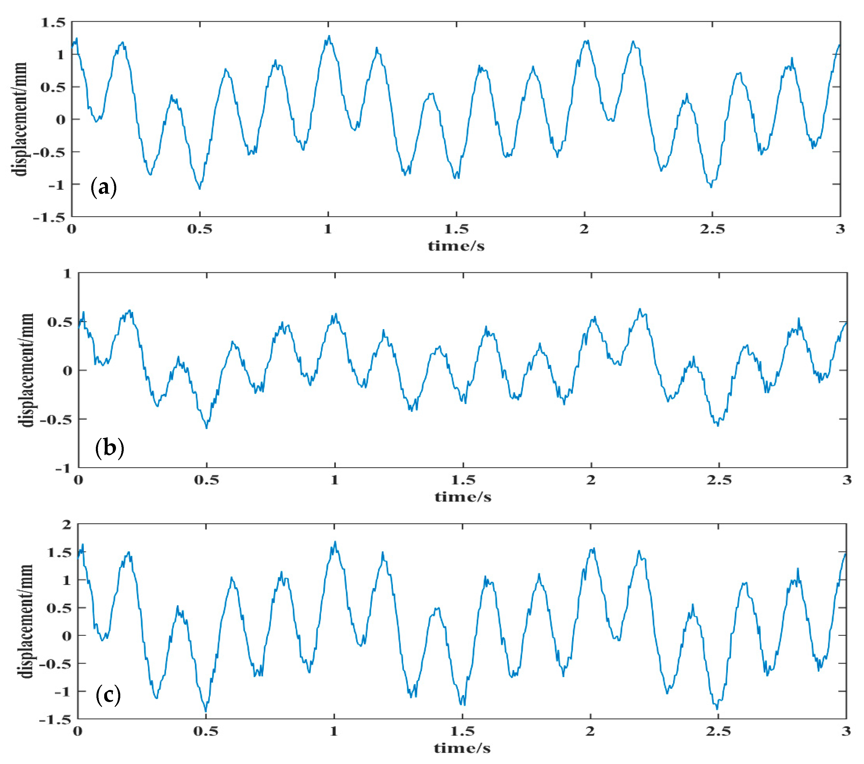
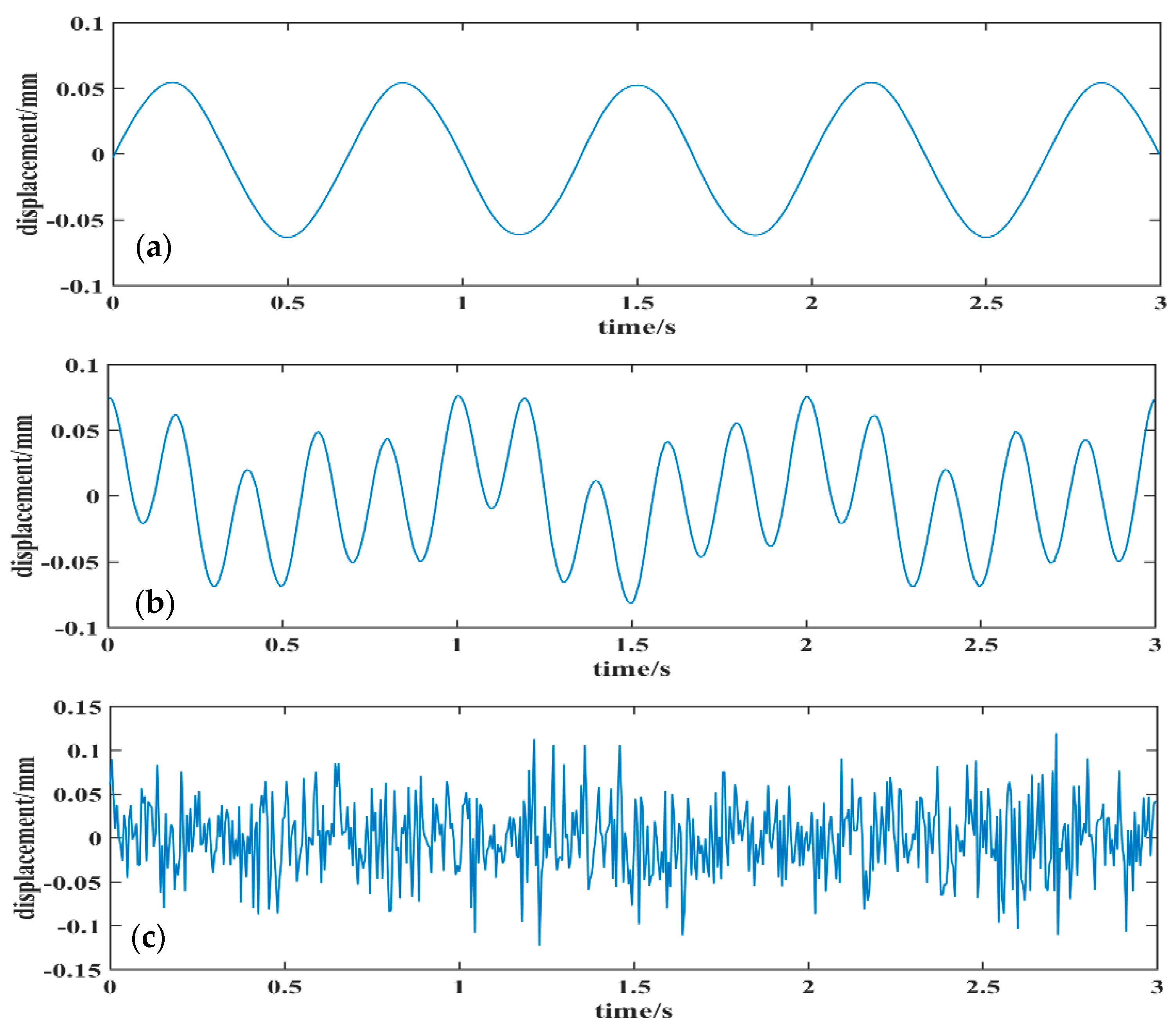
A simulation experiment was performed to validate the feasibility of the improved SOBI signal de-noising method where three mixed signals were linearly mixed using three sets of simulation source signals with different frequency scales. The obtained correlation coefficients between each simulated source signal and the corresponding separated signal component were all greater than 0.99. The results showed that the improved SOBI signal de-noising method effectively distinguished the useful signals and noise signals from the mixed signals, which can be useful for signal de-noising of time-series displacements obtained using GBSAR.

(2)

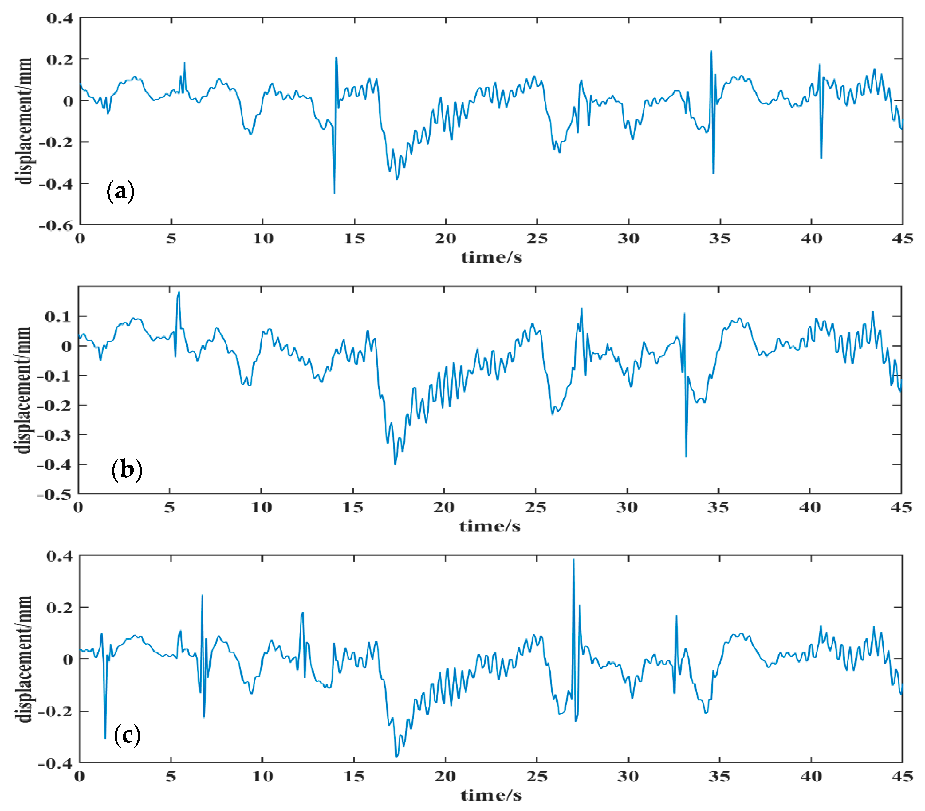
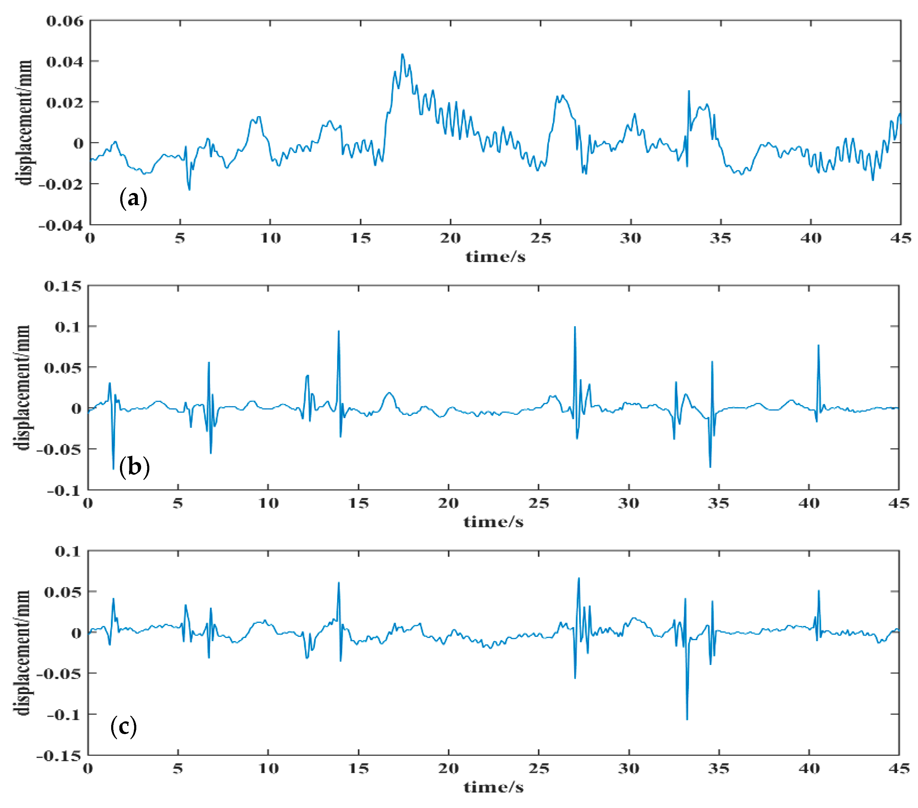
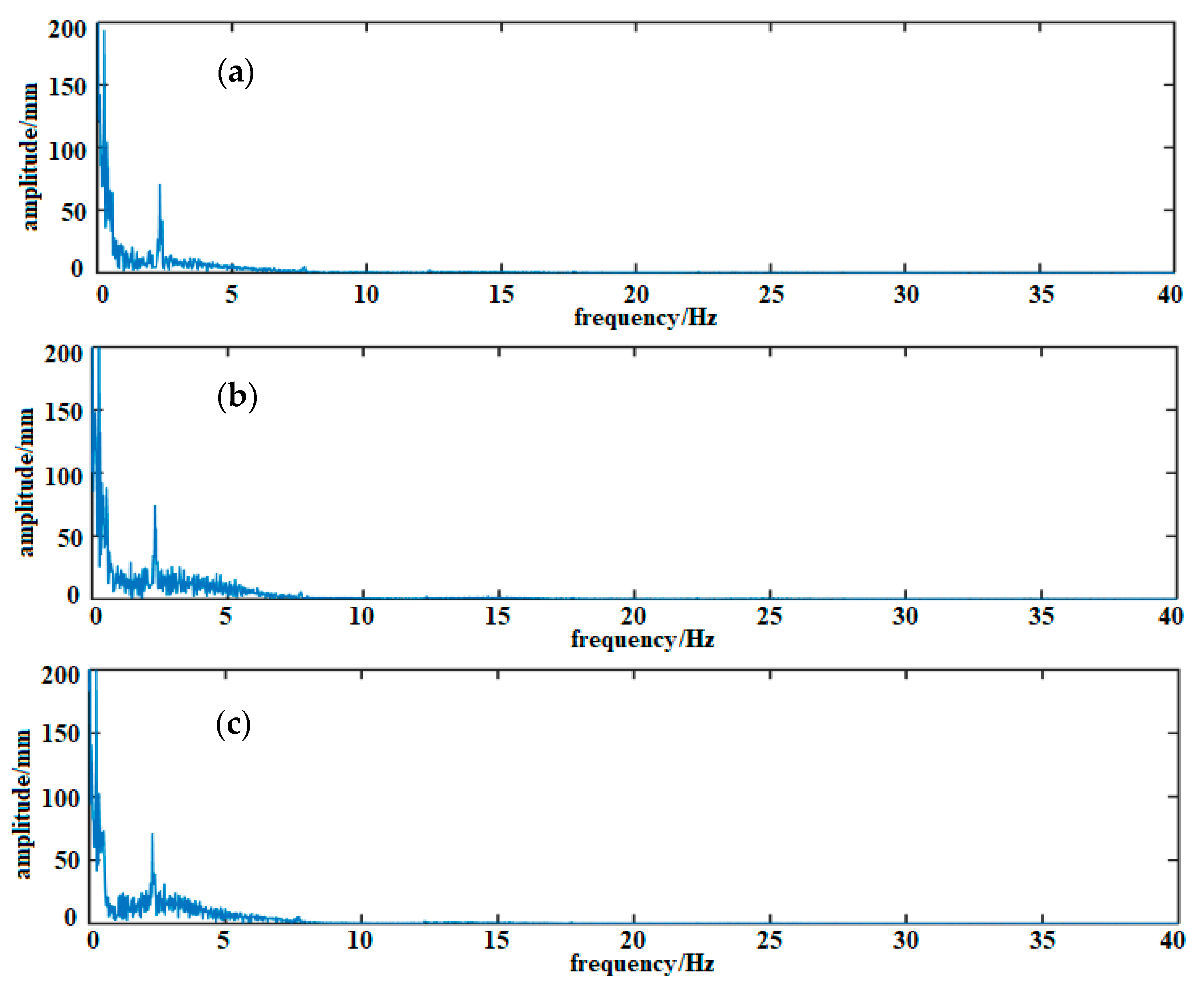
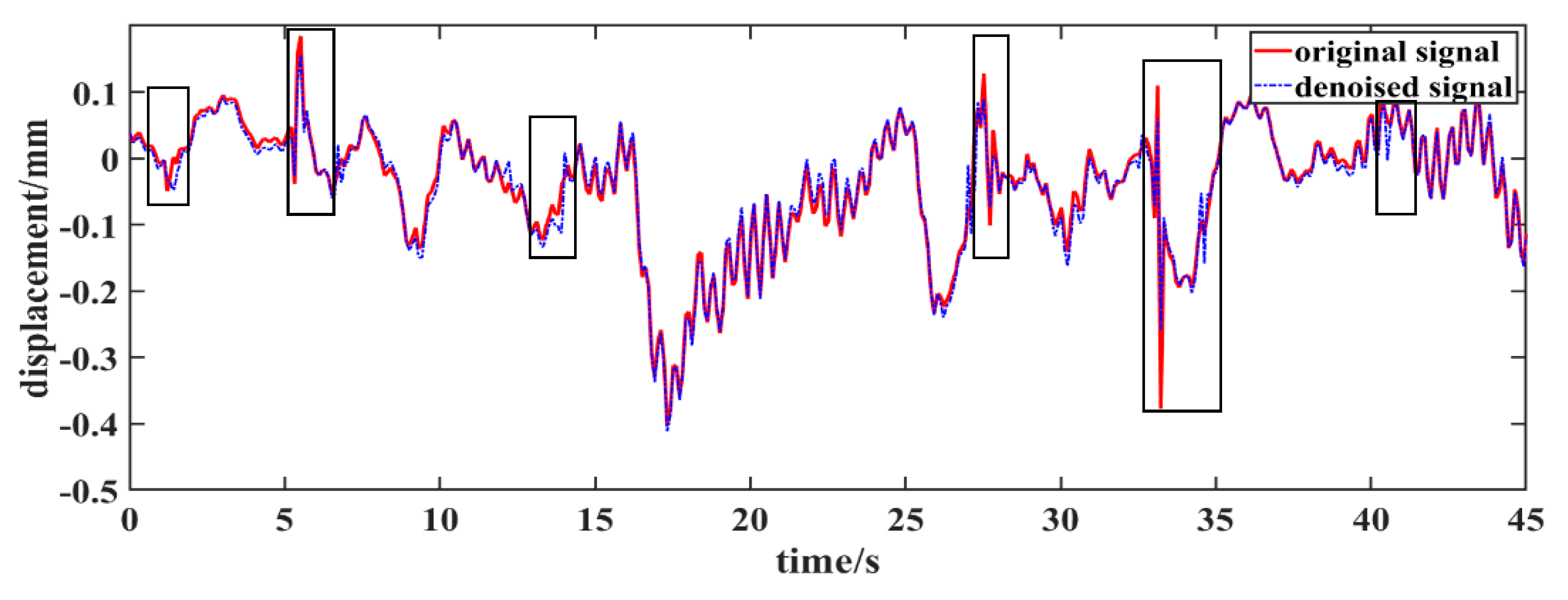
By fully considering the characteristics of the high-distance resolution GBSAR technique, the obtained dynamic time-series displacements of three adjacent monitoring points in the same time domain were selected as input signals. This was done in order to obtain the de-noised time-series displacement of the middle point among three adjacent monitoring points by using the improved SOBI signal de-noising method. Using a spectrum analysis, the separated noise components were effectively determined from the separated signals, and the original amplitude of the de-noised signal was recovered using an inverse reconstruction with a mixing matrix. The results showed that the improved SOBI signal de-noising method not only reduced the noise caused by the surrounding environment, but also reduced the noise caused by vibrations of the monitoring instrument.

(3)

Compared with the EDM and EEMD signal de-noising methods, the improved SOBI signal de-noising method displayed a greater improvement in the indexes of NRR, NM, and SER for the obtained time-series displacement of a bridge using GBSAR. The results indicate that the improved SOBI signal de-noising method has a powerful signal de-noising ability.

References

- Riveiro, B.; González-Jorge, H.; Varela, M.; Jauregui, D.V. Validation of terrestrial laser scanning and photogrammetry techniques for the measurement of vertical underclearance and beam geometry in structural inspection of bridges. Measurement 2013, 46, 784–794. [Google Scholar] [CrossRef]
- Liu, X.; Wang, P.; Lu, Z.; Gao, K.; Wang, H.; Jiao, C.; Zhang, X. Damage detection and analysis of urban bridges using terrestrial laser scanning (TLS), ground-based microwave interferometry, and permanent scatterer interferometry synthetic aperture radar (PS-InSAR). Remote Sens. 2019, 11, 580. [Google Scholar] [CrossRef]
- Monserrat, O.; Crosetto, M.; Luzi, G. A review of ground-based SAR interferometry for deformation measurement. ISPRS J. Photogramm. 2014, 93, 40–48. [Google Scholar] [CrossRef]
- Rödelsperger, S.; Läufer, G.; Gerstenecker, C. Monitoring of displacements with ground-based microwave interferometry: IBIS-S and IBIS-L. J. Appl. Geodes. 2010, 4, 41–54. [Google Scholar] [CrossRef]
- Farrar, C.R.; Darling, T.W.; Migliori, A.; Baker, W.E. Microwave interferometers for non-contact vibration measurements on large structures. Mech. Syst. Signal Process. 1999, 13, 241–253. [Google Scholar] [CrossRef]
- Granello, G.; Andisheh, K.; Palermo, A.; Waldin, J. Microwave radar interferometry as a cost-efficient method of monitoring the structural health of bridges in New Zealand. Struct. Eng. Int. 2018, 28, 518–525. [Google Scholar] [CrossRef]
- Stabile, T.A.; Perrone, A.; Gallipoli, M.R.; Ditommaso, R.; Ponzo, F.C. Dynamic survey of the musmeci bridge by joint application of ground-based microwave radar interferometry and ambient noise standard spectral ratio techniques. IEEE Geosci. Remote Sens. Lett. 2013, 10, 870–874. [Google Scholar] [CrossRef]
- Pieraccini, M.; Parrini, F.; Fratini, M.; Atzeni, C.; Spinelli, P.; Micheloni, M. Static and dynamic testing of bridges through microwave interferometry. NDT E Int. 2006, 40, 208–214. [Google Scholar] [CrossRef]
- Lim, J.S.; Oppenheim, A.V. Enhancement and bandwidth compression of noisy speech. Proc. IEEE 1979, 67, 1586–1604. [Google Scholar] [CrossRef]
- Malinowski, M.; Kwiecień, J. Study of the effectiveness of different kalman filtering methods and smoothers in object tracking based on simulation tests. Rep. Geod. Geoinformatics 2014, 97, 1–22. [Google Scholar] [CrossRef]
- Guo, X.; Shen, C.; Chen, L. Deep fault recognizer: An integrated model to denoise and extract features for fault diagnosis in rotating machinery. Appl. Sci. 2017, 7, 41. [Google Scholar] [CrossRef]
- Pan, H.X.; Men, J.F. De-noising method research on bearing fault signal based on particle filter. In Proceedings of the Second World Congress on Nature and Biologically Inspired Computing, Fukuoka, Japan, 15–17 December 2010; pp. 311–315. [Google Scholar]
- Ogundipe, O.; Lee, J.K.; Roberts, G.W. Wavelet de-noising of GNSS based bridge health monitoring data. J. Appl. Geodes. 2014, 8, 273–282. [Google Scholar] [CrossRef]
- Su, L.; Zhao, G.L. De-noising of ECG signal using translation—Invariant wavelet de-noising method with improved thresholding. In Proceedings of the IEEE Engineering in Medicine and Biology 27th Annual Conference, Shanghai, China, 17–18 January 2006; pp. 5946–5949. [Google Scholar]
- Liu, C.; Song, C.; Lu, Q. Random noise de-noising and direct wave eliminating based on SVD method for ground penetrating radar signals. J. Appl. Geophys. 2017, 144, 125–133. [Google Scholar] [CrossRef]
- Zhang, Z.; Ely, G.; Aeron, S.; Hao, N.; Kilmer, M. Novel methods for multilinear data completion and de-noising based on tensor-SVD. In Proceedings of the IEEE Conference on Computer Vision and Pattern Recognition, Columbus, OH, USA, 23–28 July 2014; pp. 3842–3849. [Google Scholar]
- Kaleem, M.F.; Guergachi, A.; Krishnan, S.; Cetin, A.E. Using a variation of empirical mode decomposition to remove noise from signals. In Proceedings of the IEEE 21st International Conference on Noise and Fluctuations, Toronto, ON, Canada, 12–16 June 2011; pp. 123–126. [Google Scholar]
- Han, G.; Lin, B.; Xu, Z. Electrocardiogram signal denoising based on empirical mode decomposition technique: An overview. J. Instrum. 2017, 12, P03010. [Google Scholar] [CrossRef]
- Huang, N.E.; Shen, Z.; Long, S.R.; Wu, M.C.; Shih, H.H.; Zheng, Q.; Yen, N.-C.; Tung, C.C.; Liu, H.H. The empirical mode decomposition and the Hilbert spectrum for nonlinear and non-stationary time series analysis. Proc. R. Soc. A 1998, 454, 903–995. [Google Scholar] [CrossRef]
- Wu, Z.; Huang, N.E. Ensemble empirical mode decomposition: A noise-assisted data analysis method. Adv. Adapt. Data Anal. 2009, 1, 1–41. [Google Scholar] [CrossRef]
- Gaci, S. A new ensemble empirical mode decomposition (EEMD) denoising method for seismic signals. Energy Procedia. 2016, 97, 84–91. [Google Scholar] [CrossRef]
- Singh, G.; Kaur, G.; Kumar, V. ECG denoising using adaptive selection of IMFs through EMD and EEMD. In Proceedings of the 2014 International Conference on Data Science & Engineering, Kochi, India, 26–28 August 2014; pp. 228–231. [Google Scholar]
- Chen, H.; Chen, P.; Chen, W.; Wu, C.; Li, J.; Wu, J. Wind turbine gearbox fault diagnosis based on improved EEMD and Hilbert square demodulation. Appl. Sci. 2017, 7, 128. [Google Scholar] [CrossRef]
- Cardoso, J.F. Blind signal separation: Statistical principles. Proc. IEEE 1998, 86, 2009–2025. [Google Scholar] [CrossRef]
- Poncelet, F.; Kerschen, G.; Golinval, J.C.; Verhelst, D. Output-only modal analysis using blind source separation techniques. Mech. Syst. Signal. Process. 2007, 21, 2335–2358. [Google Scholar] [CrossRef]
- Belouchrani, A.; Abed-Meraim, K.; Cardoso, J.F.; Moulines, E. A blind source separation technique using second-order statistics. IEEE Trans. Signal Process. 2002, 45, 434–444. [Google Scholar] [CrossRef]
- Wheland, D.; Pantazis, D. Second order blind identification on the cerebral cortex. J. Neurosci. Methods 2014, 223, 40–49. [Google Scholar] [CrossRef] [PubMed]
- Illner, K.; Miettinen, J.; Fuchs, C.; Taskinen, S.; Nordhausen, K.; Oja, H.; Theis, F.J. Model selection using limiting distributions of second-order blind source separation algorithms. Signal Process. 2015, 113, 95–103. [Google Scholar] [CrossRef]
- Gelle, G.; Colas, M.; Serviere, C. Blind source separation: A tool for rotating machine monitoring by vibrations analysis? J. Sound Vib. 2001, 248, 865–885. [Google Scholar] [CrossRef]
- Zhou, W.; Chelidze, D. Blind source separation based vibration mode identification. Mech. Syst. Signal Process. 2007, 21, 3072–3087. [Google Scholar] [CrossRef]
- McNeill, S.I.; Zimmerman, D.C. A framework for blind modal identification using joint approximate diagonalization. Mech. Syst. Signal Process. 2008, 22, 1526–1548. [Google Scholar] [CrossRef]
- Hyvärinen, A.; Oja, E. Independent component analysis: Algorithms and applications. Neural Netw. 2000, 13, 411–430. [Google Scholar] [CrossRef]
- Seppänen, J.; Turunen, J.; Koivisto, M.; Haarla, L. Measurement based analysis of electromechanical modes with Second Order Blind Identification. Electr. Power Syst. Res. 2015, 121, 67–76. [Google Scholar] [CrossRef]
- Liu, H.T.; Xie, X.B.; Xu, S.P.; Wan, F.; Hu, Y. One-unit second-order blind identification with reference for short transient signals. Inf. Sci. 2013, 227, 90–101. [Google Scholar] [CrossRef]
- Cai, J.H.; Xiao, Y.L.; Li, X.Q. Nuclear magnetic resonance logging signal de-noising based on empirical mode decomposition threshold filtering in frequency domain. Prog. Geophys. 2019, 34, 509–516. [Google Scholar]
- Lv, L.L.; Gong, W.; Song, S.L.; Zhu, B. De-noising process based on wavelet transform in feature reflectance detection LiDAR system. Geomat. Inf. Sci. Wuhan Univ. 2011, 36, 56–59. [Google Scholar]
- Lv, L.L. Evaluation system of wavelet de-noising effect for multispectral LiDAR. Hydrogr. Surv. Chart 2016, 36, 72–75. [Google Scholar]
- Liu, X.; Tong, X.; Ding, K.; Zhao, X.; Zhu, L.; Zhang, X. Measurement of long-term periodic and dynamic deflection of the long-span railway bridge using microwave interferometry. IEEE J. Sel. Top. Appl. Earth Obs. Remote Sens. 2015, 8, 4531–4538. [Google Scholar] [CrossRef]