Article

Phase Extraction from Single Interferogram Including Closed-Fringe Using Deep Learning

1
Graduate School of Engineering, Hokkaido University, Sapporo 060-8628, Japan
2
Faculty of Engineering, Hokkaido University, Sapporo 060-8628, Japan
3
Faculty of Engineering, Information and Systems, University of Tsukuba, Tsukuba 305-8573, Japan
*
Authors to whom correspondence should be addressed.
Appl. Sci. 2019, 9(17), 3529; https://doi.org/10.3390/app9173529
Submission received: 16 June 2019 / Revised: 23 July 2019 / Accepted: 23 August 2019 / Published: 28 August 2019
(This article belongs to the Special Issue Machine Learning and Compressed Sensing in Image Reconstruction)

Abstract

:
In an optical measurement system using an interferometer, a phase extracting technique from interferogram is the key issue. When the object is varying in time, the Fourier-transform method is commonly used since this method can extract a phase image from a single interferogram. However, there is a limitation, that an interferogram including closed-fringes cannot be applied. The closed-fringes appear when intervals of the background fringes are long. In some experimental setups, which need to change the alignments of optical components such as a 3-D optical tomographic system, the interval of the fringes cannot be controlled. To extract the phase from the interferogram including the closed-fringes we propose the use of deep learning. A large amount of the pairs of the interferograms and phase-shift images are prepared, and the trained network, the input for which is an interferogram and the output a corresponding phase-shift image, is obtained using supervised learning. From comparisons of the extracted phase, we can demonstrate that the accuracy of the trained network is superior to that of the Fourier-transform method. Furthermore, the trained network can be applicable to the interferogram including the closed-fringes, which is impossible with the Fourier transform method.

1. Introduction

In the last two decades, deep learning gone through a remarkable evolution, especially in image processing; for example, the classification of objects included in the image [1], noise reduction [2], pan-sharpening [3], caption generation [4] and image style transfer [5].
In this paper, we propose the method using deep learning to extract phase-shift images from a fringe patterns which is obtained from an interferometer. The extraction of the phase-shift is necessary to evaluate a refractive index of a matter of interest.
According to classical electromagnetism, the refractive indices of matters can be represented by the Drude-Lorentz model which is a spring model with dumping caused by electric dipoles and free electrons. In this model, the refractive index depends on a density of the dipoles and the free electrons. In the case of air, the density of molecules with the electric dipoles depends on temperature of the air. These relations show that a three-dimensional (3-D) temperature distribution of gas around hot matter, such as a flame, can be indirectly evaluated through a 3-D measurement of a distribution of the refractive index. As the other medium than gas, 3-D distributions of electron density in plasma and concentration of solute in solution for liquid-state media could be evaluated.
To determine the 3-D quantity, the technique of computed tomography (CT) is commonly used in medical diagnostics. In the medical CT, 2-D projection images of probe beams with different incident directions passing through a human body are measured; then, the 3-D distribution of an attenuation coefficient is reconstructed from these images. The key to the reconstruction is that the projection images include integrals of the attenuation coefficient distributed in the body along the directions of the probe beam. Upon replacing the projection from the absorption with phase-shift which is an integral of the refractive index along a path of optical beams, the 3-D refractive index can be reconstructed by the same way to the medical CT. To obtain the phase-shift caused by an object of interest, interferometer is commonly used. The authors developed a 3-D gas temperature measurement system [6,7] which uses mechanical stages to change the directions of the incident beams of the interferometer.
The first observed image by the interferometer—called an interferogram or a fringe pattern—is represented by a sinusoidal function in 2-D space of the phase-shift. To obtain the phase-shift image from the interferogram, there are two commonly used methods; the phase-shift method [8,9,10] and the Fourier-transform method [8,11,12]. The mathematical operation in the phase-shift method is simple; however, it requires the three or four interferograms for the same object with different reference phase-shift which applied one of two optical paths in the interferometer. Since the incident direction varies in the 3-D measurement system which means the object is always rotating, it is difficult to apply the phase-shift method. In contrast, the Fourier-transform method can be applied for a single interferogram. However, it requires several steps of mathematical operations: a 2-D Fourier transform, filtering in 2-D spectral domain [13,14], an inverse Fourier transform, removing background carrier pattern, and phase unwrapping [15,16,17,18,19,20], which detail processes will be shown in Section 2.
The mechanical system to control the incident direction induces vibrations of optical elements used in the system. To reduce the effect of the vibration exposure time of the camera to obtain the interferogram must be shortened. However, it causes a new problem; the obtained interferograms have much noise, which increases error to the phase-shift image at the phase unwrapping process. There is another problem in the system. The background fringe pattern cannot be controlled with high precision because the precision of the mechanical stages is dozens of times larger than the wavelength. To apply the Fourier-transform method, there is a limitation regarding the intervals of the background fringes. If the interval is too long, the fringe pattern caused by the object includes a closed-fringe pattern and the filtering process cannot be applied except in a special case [21]. In the case where the background fringe cannot be controlled, some interferograms may have closed-fringes and a complete set of the phase-shift images for CT cannot be obtained. As a result, the quality of the 3-D reconstructed distribution is reduced.
In this study, we will demonstrate the applicability of deep learning to extracting the phase-shift image from the fringe pattern even when the closed-fringe is included through a comparison to the Fourier-transform method.
The outline of this paper is as follows. In Section 2, the Fourier-transform method to extract the phase-shift image is reviewed. In Section 3, we show the phase extraction by the deep learning. The comparison of the numerical results and discussions is presented in Section 4. Finally, the summary is presented in Section 5.

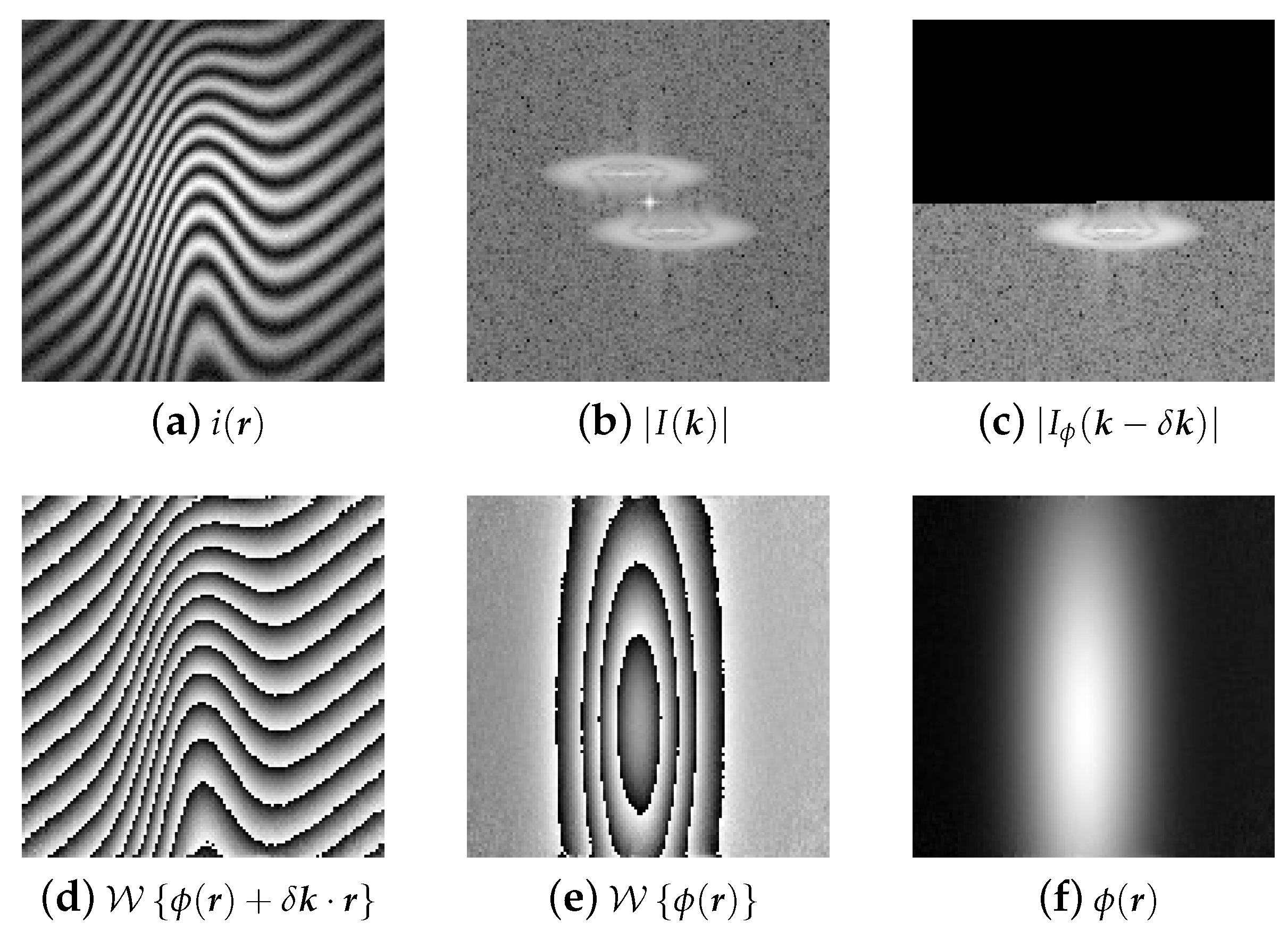
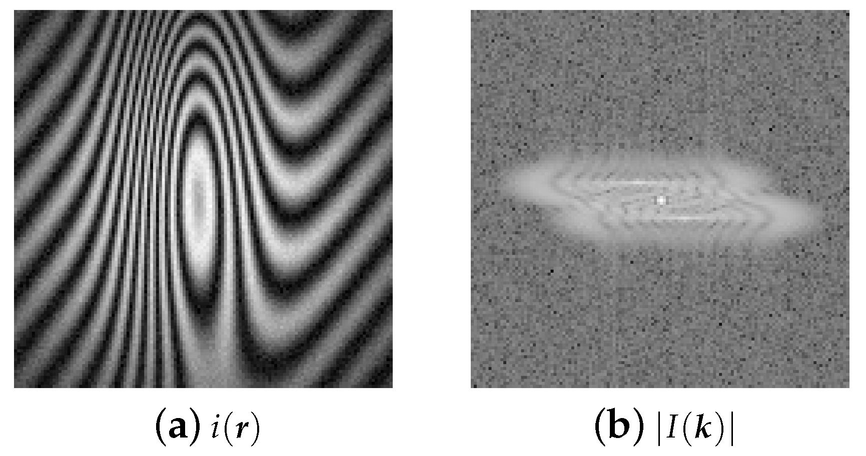
2. Fourier-Transform Method
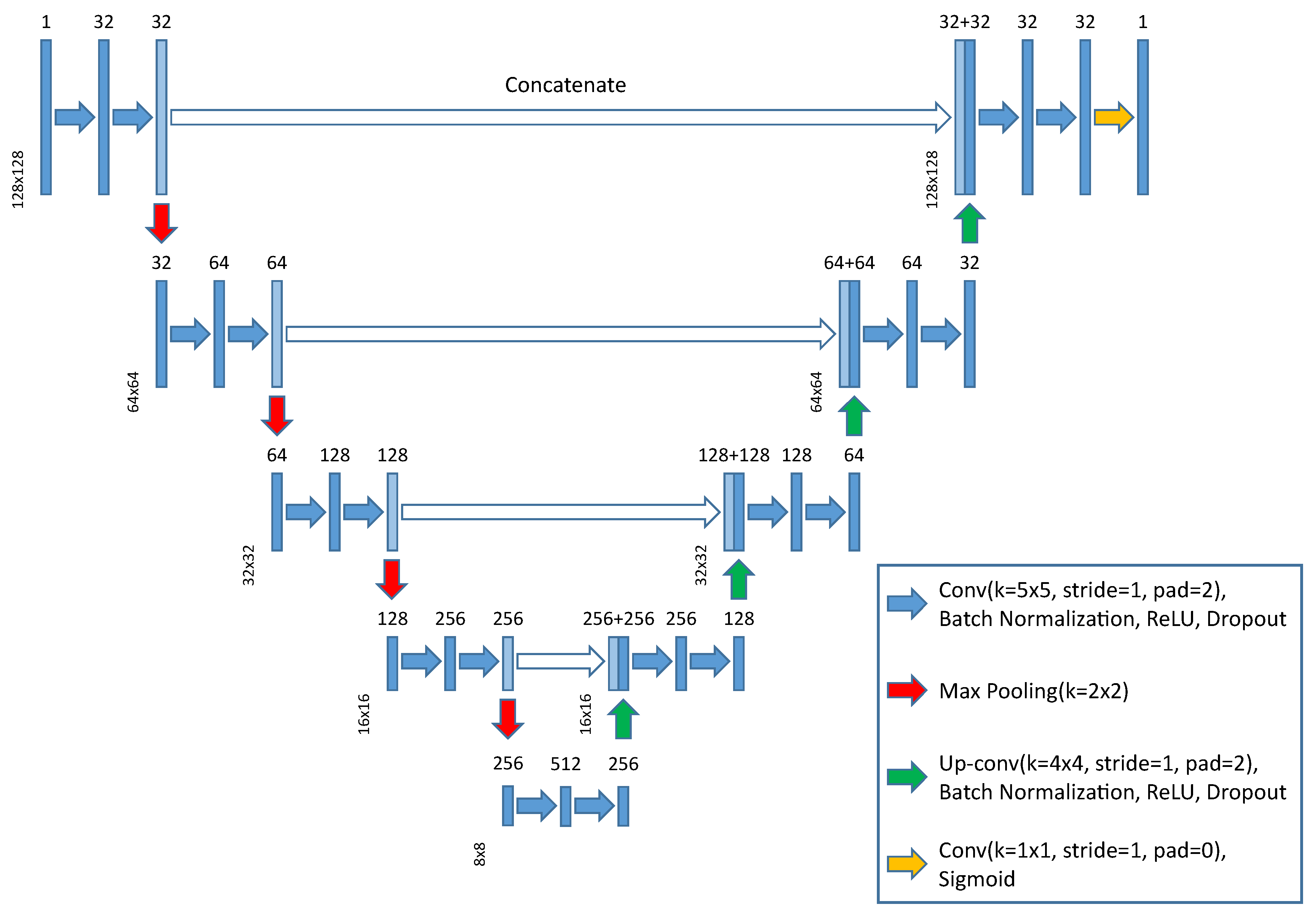
The Fourier-transform method is commonly used to obtain a phase-shift image from a single interferogram including background fringes. In this section, taking the phase extraction from the interferogram shown in Figure 1a as an example, the procedure of the Fourier-transform method is shown and the advantages and disadvantages are shown.
In the interferometer, a single optical wave is split into two waves that pass along different optical paths; one is called a reference wave which does not pass the object and the other called an object wave passing through the object with an additional phase-shift, ϕ . When their wave vectors are different but their amplitudes are provided by the same function, electric fields of both waves are expressed with the complex unit j as
E r ( r ) = E 0 ( r ) exp j k r · r ,
E o ( r ) = E 0 ( r ) exp j ( ( k r + δ k ) · r + ϕ ( r ) ) ,
where superscripts ‘ r ’ and ‘ o ’ denotes the quantities related to the reference wave and those to the object wave, respectively, and the difference of the wave vector is denoted by δ k . These waves are superposed on a screen and the interferogram, i ( r ) , is observed as a power of the superposed electric field:
i ( r ) = | E r ( r ) + E o ( r ) | 2 = 2 | E 0 ( r ) | 2 1 + cos ( ϕ ( r ) + δ k · r ) = 2 i 0 ( r ) + i ϕ ( r ) exp + j δ k · r + i ϕ * ( r ) exp j δ k · r i 0 ( r ) = | E 0 ( r ) | 2 , i ϕ ( r ) = i 0 ( r ) exp ( j ϕ ( r ) ) ,
where the symbol ‘*’ denotes a complex conjugate. To obtain the phase-shift ϕ ( r ) from this equation, the first and the last term on the right-hand side in Equation (3) can be removed by using a 2-D Fourier transform. Applying the Fourier transform to Equation (3) and using a convolutional theorem, we obtain the following equation.
I ( k ) = F i ( r ) = 2 I 0 ( k ) + I ϕ ( k δ k ) + I ϕ * ( k δ k ) , I 0 ( k ) = F i 0 ( r ) , I ϕ ( k ) = F i ϕ ( r ) ,
where F represents a 2-D Fourier transform operator. Figure 1b shows the Fourier transform of i ( r ) shown in Figure 1a. We can find three peaks in the Fourier transformed signal, I ( k ) . These peaks correspond to three terms in the right-hand side of Equation (4); the peak appearing at the center in the frequency space, k , is a DC component the distribution of which is related to the profile of the waves i 0 ( r ) , and the other two peaks spreading around k = ± δ k include the information of ϕ ( r ) related to the object. The two peaks appear point-symmetrically with respect to the origin of the frequency space. The distance between one of the two peaks and the origin represents the phase of the background fringes in the real space. This value, δ k , will be needed in subsequent procedures, and it is determined as the maximum point around peak in k -space. Next, as shown in Figure 1c, the DC component and one of the two peaks (this is referred to as a conjugate light component) is removed by filtering. To remove the DC component, we employed a method using a carrier peak isolation method [14], and to remove the conjugate component a half-plane filter [13] was employed. Thereafter, an inverse Fourier transform is applied to the filtrated image. The value of each pixel of the image obtained by this processing is represented by a complex number, which corresponds to the second term on the right-hand side in Equation (3). By taking the principal value of the logarithm of the complex number, we can obtain the following wrapped phase including the background phase, shown in Figure 1d.
W δ k · r + ϕ ( r ) = Log exp + j ( δ k · r + ϕ ( r ) ) ,
where W denotes the phase wrapping operator which returns the principal value in range [ π , + π ) . By subtracting the phase rotation caused by the background fringes, δ k · r , from the wrapped phase, the wrapped phase-shift, ϕ ( r ) , is obtained as shown in Figure 1f.
W ϕ ( r ) = W W δ k · r + ϕ ( r ) δ k · r .
This sequence of the procedures is called the Fourier-transform method. The result of the Fourier-transform method is the wrapped phase and includes the arbitrariness of an integral multiple of 2 π . To resolve the phase discontinuity, a phase unwrapping process should be applied. We employed a phase unwrapping method using localized rotational compensator [14] which is robust to the noisy wrapped phase [22].
As introduced in Section 1, there is a limitation regarding the interval of the background fringe. Since the interval in r -space is proportional to the reciprocal of | δ k | in k -space, a longer interval corresponds to a shorter | δ k | . If a width of I ϕ ( k ) is larger than the | δ k | , since I ϕ ( k δ k ) spreads to the origin, I ϕ ( k δ k ) is distorted in the filtering process of the DC peak or the conjugated peak. The carrier peak isolation method [14] can reduce the distortion; however, it cannot perfectly solve the filtering problem. The condition that I ϕ ( k δ k ) does not spread to the origin equivalent to that i ( r ) is monotonic function [21]. Otherwise, ϕ ( r ) has extrema; that is, the interferogram has closed-fringes, I ϕ ( k δ k ) spreads to the origin. Figure 2a shows examples of an interferogram including closed-fringe, and its Fourier transform is shown in Figure 2b. We can avoid this problem [21] using a coordinate-transform from the Cartesian coordinate to a polar coordinate where the origin is the extremum. However, it can only be applied in the case of a single extremum.

3. Deep Learning

In this study, we tried to introduce deep learning to phase extraction. Deep learning is the method of learning by multi-layering neural networks and has been successful in many fields, especially in the field of image processing [1]. This study uses supervised learning. Supervised learning is one of the machine learning methods and is a method for obtaining an optimal functional relation y = f ( x ) by learning a model using a large number of input data, x, and output data, y. In this study, the input, x, and the output, y, correspond to the interferograms and the phase-shift images, respectively. It should be noticed that the relations of the interferogram and the phase-shift is inverted in the physical process as an inverse problem; that is, the interferogram is the function of the phase-shift as shown in Equation (3). Since the phase-shift images have real values for each pixel, the model to be acquired is a regression model. Various models including fully convolutional networks [23] have been considered for network models in which both the input and output are an image. U-net [24] is a network originally designed for segmentation of cell images. The feature of U-net is that there are paths connecting the upstream and the downstream, and by the presence of these paths, it is possible to integrate and to learn the local features of the object and the general position information. The U-net is also used for the regression problems as a classification problem [25]. Since the extraction of the phase-shift images of the interferograms requires both local features and global position information, we adopted the same network model as U-net in this study. However, the detailed structure of each layer is different as shown in Figure 3. Specifically, the size of filters of each convolutional layer is 3 × 3 , the stride of filter applications is 1 and the spatial padding width for input arrays is 2. The size of the window of each pooling layer is 2 × 2 . Also, the size of filters of each up-convolution layer is 4 × 4 , the stride of filter applications is 1 and the spatial padding width for input arrays is 2. However, those in the final convolutional layer are 1 × 1 , 1 and 0, respectively.
It is difficult to use the measured data as the training dataset. This is because the phase-shift distribution from all measured interferograms, including those with unfavorable conditions cannot be extracted by the Fourier transform method, and in addition, it is impossible to prepare a large amount of measured data. Therefore, the pairs of the phase-shift images generated by simulation and the interferograms evaluated by them are prepared as training data.
Since the problem is the inverse problem, the output of the deep learning system, y, which is the phase-shift image, ϕ ( r ) , is defined first; then the input of the learning, x, which is the interferogram, i ( r ) , is evaluated by the simulation of interference according to Equation (3).
As a physical model, we considered a model that a probe beam with non-uniform amplitude is incident to an object which is a hot gas around candle flames. The amplitude, i 0 ( r ) , is defined by a 2-D Gaussian function and the phase-shift image, ϕ ( r ) , is also expressed by a linear combination of the 2-D Gaussian functions.
i 0 ( r ) = gauss ( r ; r i 0 , 0 , a i 0 , b i 0 ) ,
ϕ ( r ) = n ϕ n gauss ( r ; r n , θ n , a n , b n ) ,
where gauss ( ) is the 2-D Gaussian function of which contour is an ellipse:
gauss ( r ; r , θ , a , b ) = e ( r r ) T R T ( θ ) W 2 ( a , b ) R ( θ ) ( r r ) R ( θ ) = cos θ sin θ sin θ cos θ , W 2 ( a , b ) = 1 / a 2 0 0 1 / b 2 ,
where r , θ , a, and b are the center of the Gaussian function, an angle of rotation, a width in x-direction before the rotation, and that in y-direction, respectively; and the superscript T denotes a transposed matrix.
In the simulation of the interferogram, a white noise with normal distribution, i noise ( r ) , was also superposed:
i ( r ) = i 0 ( r ) ( 1 + cos ( ϕ ( r ) + δ k · r ) ) + i noise ( r ) ,
i noise ( r ) N [ 0 , σ n ] ( White , Normal ) .
In this study, 90,000 pairs of interferograms and corresponding phase-shift images were generated, of which 80,000 pairs were used as learning data and 10,000 pairs as test data.
As a learning method of the network, the back-propagation method was used.
The loss function during the training step was defined by the average of the root mean squared error of the estimated output image, ϕ DL ( r ) , from the ground truth, ϕ GT ( r ) :
E = ϕ DL ( r ) ϕ GT ( r ) 2 pixels images ,
whereas the network during and after the training was evaluated by the average of the relative root mean squared error
E ^ = ϕ DL ( r ) ϕ GT ( r ) 2 pixels / ϕ GT ( r ) 2 pixels images ,
where with a subscript denotes the average over the samples written in the subscript. The training means the iteration of updating the network parameters so that the value of the loss function E becomes smaller.

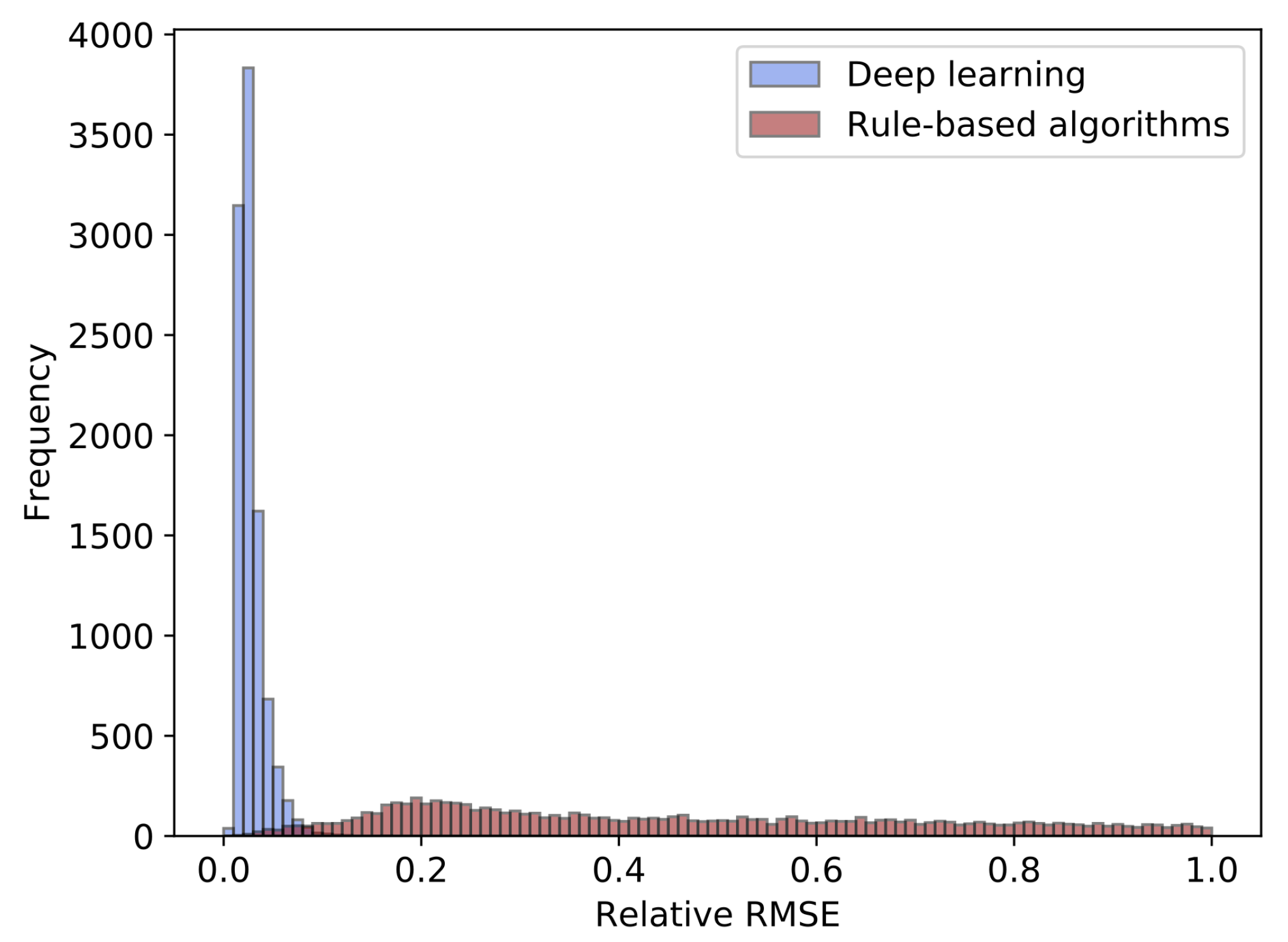
4. Results and Discussion

Figure 4 shows the evolution of the evaluation function E ^ during the learning process in the deep learning method. The vertical axis shows the evaluation function E ^ and the horizontal axis shows the epoch number. One epoch means that all training data were used once for training. The broken line shows the training data and the solid line shows the test data. We can understand that E ^ for both the training data and the test data had been decreasing monotonically during the training. In this study, batch learning was performed with a batch size of 20. Since there are 80,000 training data, 4000 relative RMSE calculations and network updates were performed for each epoch. On the other hand, in the case of the test data, 500 t of the relative RMSE calculations are performed per epoch, since the number of test data is 10,000. The dotted and solid lines of the graph indicate the average of 4000 or 500 samples calculated during the epoch, respectively. Therefore, the E ^ of the training data has a larger value than that of the test data because it contains larger error by the untrained network. Also, since we used the dropout only for the training but not for the testing, the E ^ of the training data is larger than the E ^ of the test data. Since the increase of E ^ is not found in Figure 4, the learning system is not over-learning and we can say that appropriate network models and parameters were selected. The implementation was done using Chainer, which is one of the frameworks for neural networks. A GPU was used for learning and it took about 3 h to finish 20 epochs learning.

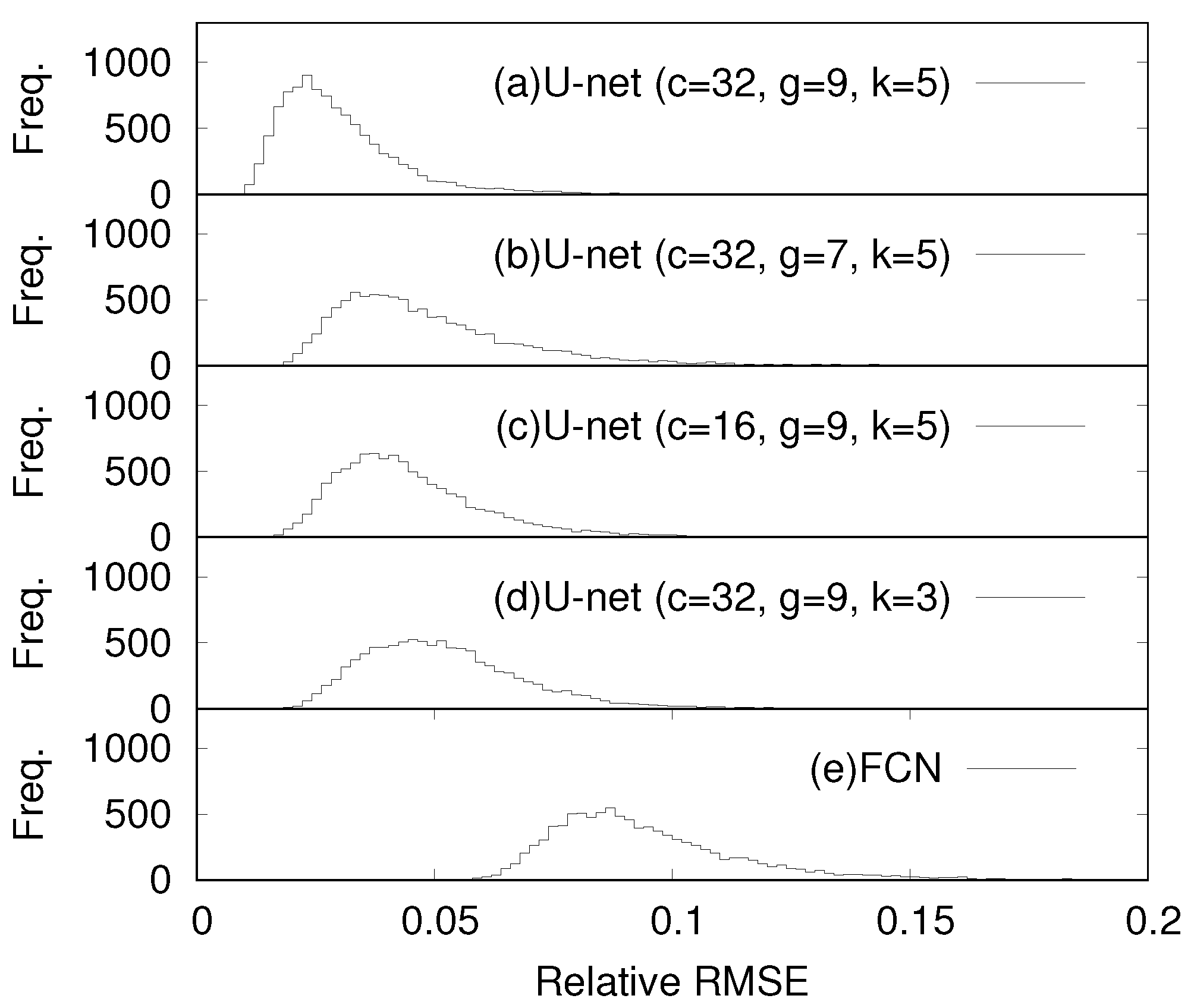
4.1. Extracted Phase-Shift from Simulated Interferogram
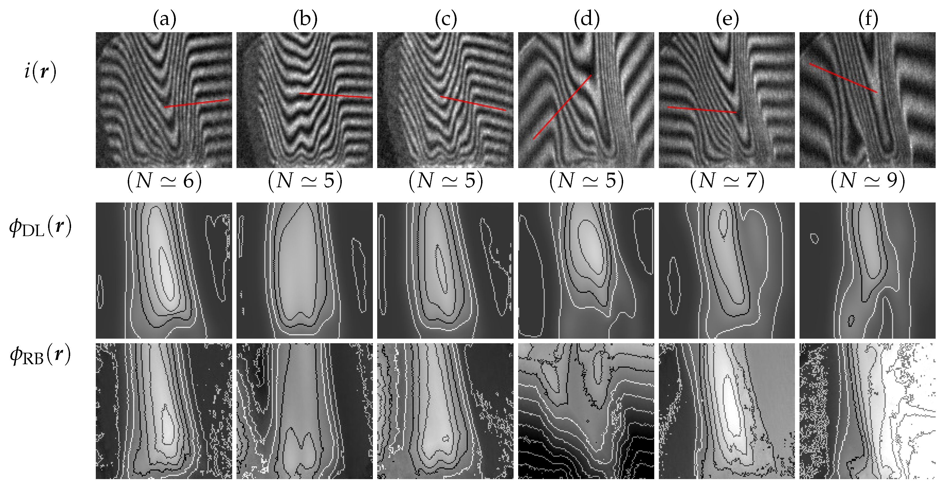
We evaluated the errors of two methods; one is the trained network and the other is the rule-based method which consists of the procedures of the Fourier-transform method and the phase unwrapping shown in Section 2. Figure 5 presents the distribution of error. The error for each image is evaluated by a relative root mean squared error defined as
e ^ = ϕ ( r ) ϕ GT ( r ) 2 pixels / ϕ GT ( r ) 2 pixels .
The most frequent error of the deep learning method is around 2% and most of the samples are distributed less than 10% error. In contrast, in case of the rule-based method, the peak is found almost 20%; furthermore, the decrease of the error is slow. In the figure, the samples with e ^ > 1 . 0 (100%) are omitted and they are excluded in the evaluation of the error average, which will be shown below, the number of those samples reaches almost 2000 among 10,000 test data. The average of e ^ using the trained network is 0.027, meanwhile that using the rule-based algorithms is 0.455. The error of the rule-based algorithm is almost twenty times larger than that of the deep learning, despite excluding the samples with enormous errors by the rule-based algorithm. From this comparison it is evident that phase extraction from interferograms by using the deep learning is superior to that using the rule-based algorithms.
The correlation of the extraction error between the two methods is shown in Figure 6. We can understand that there are no correlations between the rule-based algorithm and the deep learning. It means that the reasons of the error are different, and the interferogram which causes large error to the phase are different.
Figure 7 presents comparisons between the extracted phases by the deep learning and that by the Fourier-transform methods for typical interferograms;
(a):
the estimation errors, E ^ , by both the deep learning and the Fourier-transform method from the interferogram, i ( r ) , belong to the maximum of the histogram shown in Figure 5; which are called a mode,
(b):
E ^ of the Fourier-transform method is smaller than the mode, E ^ by both the deep learning and the rule-based algorithm are the mode of the histogram shown in Figure 5,
(c):
and (d): the interferograms include closed-fringes.
The interferograms, i ( r ) , shown in the figure are some of the test data, which were not used for training in the deep learning method. In the case of results from the deep learning, ϕ DL , we cannot find the significant difference of i ( r ) from the images, since their errors are sufficiently small.
For the case of the rule-based algorithm, we can find that the interferograms, i ( r ) , shown in (c) and (d) includes closed-fringe, and their results, ϕ RB , include large error as predicted in Section 2. Between these two, the error of (d) is larger than (c), and the number of closed-fringes has the same relation. Therefore, the closed-fringe strongly reduces the accuracy. Both i ( r ) in (a) and (b) do not include the closed-fringes; however, there is a difference between the error of them. The reason for the difference is caused by the size of area with small phase value, of which pixels are depicted by dark pixels in ϕ GT . The area with small phase in (a) is smaller than (c). In the Fourier-transform method the carrier frequency, δ k , is important, if it has error, Δ δ k , the error of the phase, Δ ϕ , spread to whole image as a planar (linear in 2-D space) function with a constant gradient as
Δ ϕ ( r ) = Δ δ k · r ,
As mentioned in Section 2, δ k is determined from the peak position in k -space. When the non-zero phase area spread to whole image, an intensity of the peak caused by δ k becomes smaller and δ k may not be detected. From ϕ RB in (a), a leftward phase gradient is observed on both sides of the image. Similar to (a), ϕ RB in (b) a rightward smaller gradient is also observed. These errors can be compensated after the phase extraction. However, the case of the closed-fringe cannot be compensated the error.
As discussed in this section, the rule-based algorithm has many factors to induce the phase error. In contrast, once the trained network with appropriate parameters is acquired, the phase is extracted accurately. Deep learning is especially applicable to the interferogram including the closed-fringe, which cannot be solved by the Fourier-transform method.
These results show that the phase extraction from the simulated interferograms using deep learning was successful and better than the rule-based algorithms.
As some comparisons, the results of U-nets with different parameters and an FCN are shown. The Figure 8 shows the histograms similar to the Figure 4, and they represent the extraction accuracy from each network. The U-net of (a) is the same as that of the Figure 3. The U-nets from (b) to (d) are the ones with the following parameters changed from (a). The parameter c is the number of output channels in the first convolutional layer, g is the number of groups that make up U-net when two consecutive convolutional layers are regarded as one group, and k is the kernel size of each convolutional layer. The parameters of (a) are c = 32 , g = 9 , and k = 5 , whereas (b) is g = 7 , (c) is c = 16 , and (d) is k = 3 . In addition to these, (e) FCN was prepared, which has almost the same learning time as (c) U-net. From the results of Figure 8, it can be said that U-net is suitable for the phase extraction problem. Further, it can be expected that the extraction accuracy will be further improved by increasing the parameters c, g and k but the learning cost will be increased accordingly. Since the average of relative RMSE when using (a) is about 0.027 and the accuracy is sufficient, the U-net used in this paper is optimal for the phase extraction problem.

4.2. Extracted Phase-Shift from Interferogram Obtained by an Experiment

In order to demonstrate the validity of the deep learning method in the phase extraction estimation from the interferograms, we applied the algorithms to interferograms which are obtained by an experiment to measure a 3D refractive index distribution in which the object is three candle flames [7]. Figure 9 shows triplets of an interferogram, i ( r ) , and the extracted phase-shifts by two methods; one is the deep learning, ϕ DL ( r ) , and the other is the rule-based method, ϕ RB ( r ) , where the rule-based method is a set of sequential procedures of the Fourier-transform method and the phase unwrapping process of which detail is shown in Section 2. The extracted phase obtained by the rule-based method can be the true solution, if condition of the interferogram is good. However, the interferograms shown in Figure 9 have high density of the fringes and include much noise. In this condition, the results include much error. To evaluate the accuracy we roughly estimated the phase-shift at a sampling point by counting the number of fringes across a reference line which is parallel to the background fringe. The reference lines are drawn with red color in i ( r ) in Figure 9 and the estimated number of fringes are shown as N below i ( r ) . Since the interval between fringes in the interferogram is 2 π , the number of fringes crossing the reference line is equal to the phase-shift divided by 2 π . By counting the number of contour lines from background to the point of interest, ϕ DL ( r ) and ϕ RB ( r ) in (a)–(d) are almost equal to N. However, the distorted phase distributions are found ϕ RB ( r ) in (b) and (c) where the fringes are not found in i ( r ) . In the deep learning method, we can assume that there no phase-shift at both sides by the learning data. In contrast, the rule-based cannot generally impose this condition. In (d), ϕ RB ( r ) show unnatural distribution caused by the dense fringes. From these results, the phase-shift estimated by the deep learning seems to good performance similar to the previous subsection. However, the deep learning method sometimes returns incorrect estimation which are shown in (e) and (f). In both cases the phase-shifts are underestimated in ϕ D L ( r ) . In i ( r ) in (e) and (f) includes dense and unclear fringes.

5. Conclusions

In this study, we have introduced deep learning to extract phase-shift images from single-shot interferograms. A large amount of interferograms and their corresponding phase-shift images were prepared by simulation, and deep neural networks with them as input and output, respectively, were trained by supervised learning. The learned network showed higher performance in phase extraction from unknown interferograms than the Fourier-transform method which is conventional phase extraction method. In addition, even when the interferogram includes closed ring-shaped fringes, the deep learning can extract the phase-shift without decreasing accuracy; in contrast, the Fourier-transform method includes much error. From these results, we can conclude that deep learning is useful for phase extraction from interferograms than the Fourier-transform method. However, we cannot determine the accuracy for arbitrary interferograms, since the performance is evaluated for the cases where the true solutions are known. If the actual experimental data is far from the data used in the supervised learning, the accuracy might be worse. In such cases, we should tune the algorithm to generate the output of supervised learning. Therefore, we leave to be considered about the interferogram generation model that more closely reflects the measurement conditions such as distortion due to the aberration of the interferometer lens, or the phase-shift generation model using some distribution other than Gaussian distribution; however, we cannot determine whether the experimental data is far from the supervised learning data set or not. The next task with high priority will be development of scheme to evaluate the accuracy of the output from the trained network for arbitrary input.

Author Contributions

Conceptualization, D.K.; Methodology, D.K.; Software, D.K., S.T. and N.M.; Validation, D.K and R.U.; Formal analysis, D.K.; Investigation, D.K. and R.U.; Resources, S.T.; Data curation, D.K., S.T. and N.M.; Writing–original draft preparation, D.K. and S.T.; Writing–review and editing, D.K. and S.T.; Visualization, D.K. and S.T.; Supervision, S.T.; Project administration, S.T.; Funding acquisition, S.T.

Funding

This research was funded by Japan Society for the Promotion of Science KAKENHI grant number 18K04158.

Conflicts of Interest

The authors declare no conflict of interest.

References

  1. Krizhevsky, A.; Sutskever, I.; Hinton, G.E. Imagenet classification with deep convolutional neural networks. In Proceedings of the Advances in Neural Information Processing Systems, Lake Tahoe, NV, USA, 3–6 December 2012; pp. 1097–1105. [Google Scholar]
  2. Zhang, K.; Zuo, W.; Chen, Y.; Meng, D.; Zhang, L. Beyond a gaussian denoiser: Residual learning of deep cnn for image denoising. IEEE Trans. Image Process. 2017, 26, 3142–3155. [Google Scholar] [CrossRef]
  3. Huang, W.; Xiao, L.; Wei, Z.; Liu, H.; Tang, S. A new pan-sharpening method with deep neural networks. IEEE Geosci. Remote Sens. Lett. 2015, 12, 1037–1041. [Google Scholar] [CrossRef]
  4. Vinyals, O.; Toshev, A.; Bengio, S.; Erhan, D. Show and tell: A neural image caption generator. In Proceedings of the IEEE Conference on Computer Vision and Pattern Recognition, Boston, MA, USA, 7–12 June 2015; pp. 3156–3164. [Google Scholar]
  5. Gatys, L.A.; Ecker, A.S.; Bethge, M. A neural algorithm of artistic style. arXiv 2015, arXiv:1508.06576. [Google Scholar] [CrossRef]
  6. Tomioka, S.; Nishiyama, S.; Heshmat, S.; Hashimoto, Y.; Kurita, K. Three-dimensional gas temperature measurements by computed tomography with incident angle variable interferometer. Proc. SPIE 2015, 9401, 94010J. [Google Scholar] [CrossRef]
  7. Tomioka, S.; Nishiyama, S.; Miyamoto, N.; Kando, D.; Heshmat, S. Weighted reconstruction of three-dimensional refractive index in interferometric tomography. Appl. Opt. 2017, 56, 6755–6764. [Google Scholar] [CrossRef] [PubMed]
  8. Perry, K.E., Jr.; McKelvie, J. A Comparison of Phase Shifting and Fourier Methods in the Analysis of Discontinuous Fringe Patterns. Opt. Lasers Eng. 1993, 19, 269–284. [Google Scholar] [CrossRef]
  9. Bruning, J.H.; Herriott, D.R.; Gallagher, J.E.; Rosenfeld, D.P.; White, A.D.; Brangaccio, D.J. Digital Wavefront Measuring Interferometer for Testing Optical Surfaces and Lenses. Appl. Opt. 1974, 13, 2693–2703. [Google Scholar] [CrossRef]
  10. Breuckmann, B.; Thieme, W. Computer-aided analysis of holographic interferograms using the phase-shift method. Appl. Opt. 1985, 24, 2145–2149. [Google Scholar] [CrossRef]
  11. Takeda, M.; Ina, H.; Kobayashi, S. Fourier-transform method of fringe-pattern analysis for computer-based topography and interferometry. J. Opt. Soc. Am. 1982, 72, 156–160. [Google Scholar] [CrossRef]
  12. Cuche, E.; Marquet, P.; Depeursinge, C. Spatial Filtering for Zero-Order and Twin-Image Elimination in Digital Off-Axis Holography. Appl. Opt. 2000, 39, 4070–4075. [Google Scholar] [CrossRef]
  13. Bone, D.J.; Bachor, H.A.; Sandeman, R.J. Fringe-pattern analysis using a 2-D Fourier transform. Appl. Opt. 1986, 25, 1653–1660. [Google Scholar] [CrossRef]
  14. Tomioka, S.; Nishiyama, S.; Heshmat, S. Carrier peak isolation from single interferogram using spectrum shift technique. Appl. Opt. 2014, 53, 5620–5631. [Google Scholar] [CrossRef] [PubMed]
  15. Fried, D.L. Least-square fitting a wave-front distortion estimate to an array of phase-difference measurements. J. Opt. Soc. Am. 1977, 67, 370–375. [Google Scholar] [CrossRef]
  16. Goldstein, R.M.; Zebker, H.A.; Werner, C.L. Satellite radar interferometry: Two-dimensional phase unwrapping. Radio Sci. 1988, 23, 713–720. [Google Scholar] [CrossRef] [Green Version]
  17. Flynn, T.J. Two-dimensional phase unwrapping with minimum weighted discontinuity. JOSA A 1997, 14, 2692–2701. [Google Scholar] [CrossRef]
  18. Tomioka, S.; Heshmat, S.; Miyamoto, N.; Nishiyama, S. Phase unwrapping for noisy phase maps using rotational compensator with virtual singular points. Appl. Opt. 2010, 49, 4735–4745. [Google Scholar] [CrossRef] [PubMed]
  19. Heshmat, S.; Tomioka, S.; Nishiyama, S. Reliable phase unwrapping algorithm based on rotational and direct compensators. Appl. Opt. 2011, 50, 6225–6233. [Google Scholar] [CrossRef]
  20. Tomioka, S.; Nishiyama, S. Phase unwrapping for noisy phase map using localized compensator. Appl. Opt. 2012, 51, 4984–4994. [Google Scholar] [CrossRef]
  21. Ge, Z.; Kobayashi, F.; Matsuda, S.; Takeda, M. Coordinate-Transform Technique for Closed-Fringe Analysis by the Fourier-Transform Method. Appl. Opt. 2001, 40, 1649–1657. [Google Scholar] [CrossRef]
  22. Heshmat, S.; Tomioka, S.; Nishiyama, S. Performance Evaluation of Phase Unwrapping Algorithms for Noisy Phase Measurements. Int. J. Optomech. 2014, 8, 260–274. [Google Scholar] [CrossRef] [Green Version]
  23. Long, J.; Shelhamer, E.; Darrell, T. Fully convolutional networks for semantic segmentation. In Proceedings of the IEEE Conference on Computer Vision and Pattern Recognition, Boston, MA, USA, 7–12 June 2015; pp. 3431–3440. [Google Scholar]
  24. Ronneberger, O.; Fischer, P.; Brox, T. U-net: Convolutional networks for biomedical image segmentation. In Proceedings of the International Conference on Medical Image Computing and Computer-Assisted Intervention, Shenzhen, China, 13–17 October 2015; Springer: Cham, Switzerland, 2015; pp. 234–241. [Google Scholar]
  25. Yao, W.; Zeng, Z.; Lian, C.; Tang, H. Pixel-wise regression using U-Net and its application on pansharpening. Neurocomputing 2018, 312, 364–371. [Google Scholar] [CrossRef]
Figure 1. An example of processing of Fourier-transform method: (a) interferogram, i ( r ) . (b) | I ( k ) | : absolute value of Fourier transform of (a) where the origin in k -space is located at the center of the image and the brightness of the image is shown with logarithm scale. The distribution I ( k ) is superposed results of three peaks; one is a DC-peak at the origin, the other two are the spreading distribution around the carrier peak and its complex conjugate. (c) | I ϕ ( k δ k ) | : filtered Fourier spectrum around the carrier peak, δ k . (d) W ϕ ( r ) + δ k · r : wrapped phase with carrier-shift obtained by evaluation of an angle of complex value at each point on inverse Fourier transformed image of (d). (e) W ϕ ( r ) : wrapped phase-shift after cancellation of carrier frequency. (f) ϕ ( r ) : unwrapped phase-shift.
Applsci 09 03529 g001
Figure 2. Interferogram including closed-fringe and overlapping of Fourier transformed peak. The meanings of (a,b) are the same as those in Figure 1. It is difficult to filter the carrier peak, since the boundaries of the three peaks are not clear.
Applsci 09 03529 g002
Figure 3. Architecture of U-net used in this study. Each blue box represents a multi-channel feature map. The number of channels is shown at the top of the box. The size of the image is described at the lower left of the box. The white right pointing arrow indicates copy of the box on the left-hand side to that on the right-hand side. The other four colored arrows mean different operations.
Applsci 09 03529 g003
Figure 4. Evolution of the evaluation function E ^ . The horizontal axis indicates the epoch number, and the vertical axis indicates the evaluation function E ^ . Training data represents the data used for the training and test data represent the data not used for the training.
Applsci 09 03529 g004
Figure 5. Distribution of the root mean squared error, E ^ , by the deep learning and the rule-based algorithms for 10,000 test data. The data which have the relative root mean squared error of more than 1.0 are not shown.
Applsci 09 03529 g005
Figure 6. Correlation of errors between the deep learning and the rule-based method. Both the axes represent the relative error defined in Equation (14).
Applsci 09 03529 g006
Figure 7. Examples of extracted phase-shift and relative error. Four different sample data are shown as (ad). The images in the first column, i ( r ) , are interferograms which are input to the phase extraction methods. The images in the second column, ϕ GT is the grand true phase which is used to prepare i ( r ) as a forward simulation. The remained two columns are of the phase-shift images estimated by the deep learning, ϕ DL , and that by the rule-based algorithm, ϕ RB .
Applsci 09 03529 g007
Figure 8. Distributions of the relative root mean squared error, by the various U-nets and an FCN for 10,000 test data. The parameter c is the number of output channels in the first convolutional layer, g is the number of groups that make up U-net when two consecutive convolutional layers are regarded as one group, and k is the kernel size of each convolutional layer.
Applsci 09 03529 g008
Figure 9. Examples of extracted phase-shift from experimental interferograms. Six different sample data are shown as (af). The images in the first row, i ( r ) , are interferograms which are input to the phase extraction methods. The red line segment in each i ( r ) indicates a reference line to count the number of fringes from background area manually. The counted number of fringes along the line segment, N, is shown below i ( r ) . The second and third rows are the phase-shift images estimated by the deep learning, ϕ DL , and that by the rule-based algorithm, ϕ RB , respectively. In each figure, the curved lines depict contour lines of the phase-shift with intervals 2 π . The size of images is 128 × 128 pixels.
Applsci 09 03529 g009

