Use of a Weighted ICP Algorithm to Precisely Determine USV Movement Parameters

Abstract

The purpose of this article is to present a study aimed at developing a method for the precise determination of unmanned surface vehicle (USV) movement parameters (heading (HDG), speed over ground (SOG) and rate of turn (ROT)) through appropriate processing. The technique employs a modified weighted ICP (Iterative Closest Point) algorithm and a 2D points layer arranged in the horizon plane obtained from measurements. This is performed with the help of Light Detection and Ranging (LIDAR). A new method of weighting is presented. It is based on a mean error in a given direction and the results of modified weighted ICP tests carried out on the basis of field measurement data. The first part of the paper characterizes LIDAR measuring errors and indicates the possibilities for their use in matching point clouds. The second part of the article deals with a method for determining the SOG and course over ground (COG), based on a modified weighted ICP algorithm. The main part of the paper reviews a test method aimed at evaluating the accuracy of determining the SOG and COG by the scan-matching method using a modified weighted ICP algorithm. The final part presents an analysis comparing the obtained SOG and COG results with reference results of GNSS RTK measurements and the resulting generalised conclusions.

1. Introduction

Heading (HDG), speed over ground (SOG) and rate of turn (ROT) are basic movement parameters which characterize the way a ship’s hull moves in relation to the Earth’s surface. They are crucial in the decision-making process, particularly when navigating in congested areas, including harbors and rivers. Currently, these parameters are most frequently determined on a ship using a gyrocompass and a log, i.e., navigational instruments whose measuring accuracy, according to the International Maritime Organization (IMO) requirements, is not required to be very high: “Errors in the indicated speed, when the ship is operating free from shallow water effect and from the effects of wind, current and tide, should not exceed 2% of the speed of the ship, or 0.2 knots, whichever is greater” [1], “The follow-up error for different rates of turn should be: less than ±0.5° at rates up to 10°/s; and less than ±1.5° between a rate of 10°/s and 20°/s” [2], although it determines the precision and the ability to control the ship’s movement which, consequently, may affect the navigational safety level. It is therefore reasonable to carry out scientific research aimed at searching for new measuring and data processing methods in order to minimize measuring errors in a ship’s movement parameters.

For many years, maritime navigation has placed increasing emphasis on the development of methods to determine position and navigational parameters that could offer an alternative to the GNSS system [3]. In the age of the development of unmanned surface vehicles (USVs) whose main tasks increasingly involve independent (autonomous) maneuvering in restricted areas, it is necessary to develop new methods to obtain precise (accurate) navigational movement parameters (in particular the HDG, SOG, course over ground (COG), and ROT) [4,5]. Basing the USV decision-making process exclusively on the parameters of movement and positions obtained from satellite systems is unjustified, particularly in port basins in which infrastructure facilities and other ships may suppress and reflect the system signals [6,7,8]. Another reason why one should not rely exclusively on such solutions is the new techniques of satellite signal jamming and spoofing [9].

A good way to avoid the satellite system inconveniences may be the development of locally operating systems whose actuator is located on a carrier ship, making their operation more difficult to interfere with. A system with a local range of operation needs no special, external infrastructure to generate correct data. Recently, the clear development of devices such as Light Detection and Ranging (LIDAR) [10] has been noted, with increased capacities in terms of the range, accuracy of generated data and the purchase price. Certain devices have a range above 500 m and high accuracy in angle and distance measurements, which enables more widespread use of such devices in sea-going ship navigation. It should also be noted that the measuring capacity of such sensors is not limited by the radar’s dead zone at close ranges. On the other hand, such a phenomenon is typical of pulse radars which are commonly used on almost every vessel [11].

This article presents a method for the precise determination of the SOG and COG parameters through processing, using a modified iterative closest point (ICP) algorithm [12,13,14,15] of a horizontal 2D layer of cloud points obtained from LIDAR measurements. The main process is based on the simultaneous localization and mapping (SLAM) method. In simple terms, this is a method allowing a map of an unknown environment to be built, which, after processing, is used for navigating in a particular area. This technique was isolated as a separated area of interest in 1996. The SLAM evolution was described in [16]. SLAM is rarely used in determining the position of surface vessels. Only a few applications of the method in the context of its use on an open sea surface are known [17]. On the other hand, SLAM has become very popular in determining the position of autonomous underwater vehicles (AUV). A review of the methods applied in determining the positions of AUVs can be found in [18]. Since SLAM is already a relatively well-studied method, many approaches to solving a particular position-determining problem have emerged. One of the most common solutions to the problem is the so-called scan-matching. This set of techniques involves matching the subsequent scans of the surrounding environment which are obtained while exploring a particular area [19]. There are numerous algorithms variants used to match scans obtained by mapping devices. These include the ICP algorithm [20,21], ICL [22] and algorithms based on matching histograms of the distance function [23]. However, given the different methods of matching point clouds, the ICP algorithm proposed for the first time in [24] outperforms other algorithms in its simplicity and the possibility for its continuous development.

Considering the use of the SLAM technique to determine the parameters of the vessel’s movement, it is worth looking at the 2011 article by Callmer et al. [25]. In this case, the authors use the object approach (landmark) based on the SIFT algorithm and the extended Kalman filter (EKF), and images from the navigation radar. The results of the work are promising; however, in this case there is a significant drift of coordinates of the position and parameters of the vessels movement. Another publication describing the implementation of the SLAM task at sea [17]. The approach presented here assumes that the map of the environment will be explored on a simultaneous basis by more than one vehicle/ship. This assumption allows obtaining a much more accurate model of the map of the environment (global map) by combining many sub-maps obtained by vehicles. This mapping is used to position each of them.

The approach presented in the article is a scan matching without odometry information. A similar solution, but based on another scan matching algorithm, was presented in [26]. It involves adjusting concurrent scans one after another without using dead reckoning data in the alignment algorithm. This article uses the ICP algorithm with the error metric in the point-to-point version [27]. Other versions of the metrics are: point-to-line [28], point-to-plane [29], and plane-to-plane [30]. The point-to-point metric was chosen because of the intuitive way of attaching importance to individual correspondences (based solely on the coordinate error of the position of a pair of points), without the need to consider the uncertainty of the position of the line or plane (for cases of three-dimensional point clouds).

In this article, the emphasis is put on the methods of weighting on the basis of estimated errors of the position coordinates of a pair of corresponding points. The problem of weighting of pairs in a navigational approach is presented in [31], and for other applications in [32,33]. This publication assumes that pairs with a higher distance value between points will be given lower weights compared to those at a smaller distance from one another. Weighting based on color was also accepted. Another approach presented in [21] is the weighting depending on the uncertainty of the position of points in the scan and the uncertainty of the position of the straight line (in the point-to-line variant). It was assumed that more weight will be put on pairs that have less influence on the error metric. A similar approach is presented in [34]. The authors carry out tests on three variants of the error measure: point, line and plane. The approach proposed in this article is similar to this; however, it assumes a different, more universal distribution of coordinates error. They can be easily implemented not only in the case of a lidar sensor, but also in the case of navigation radar.

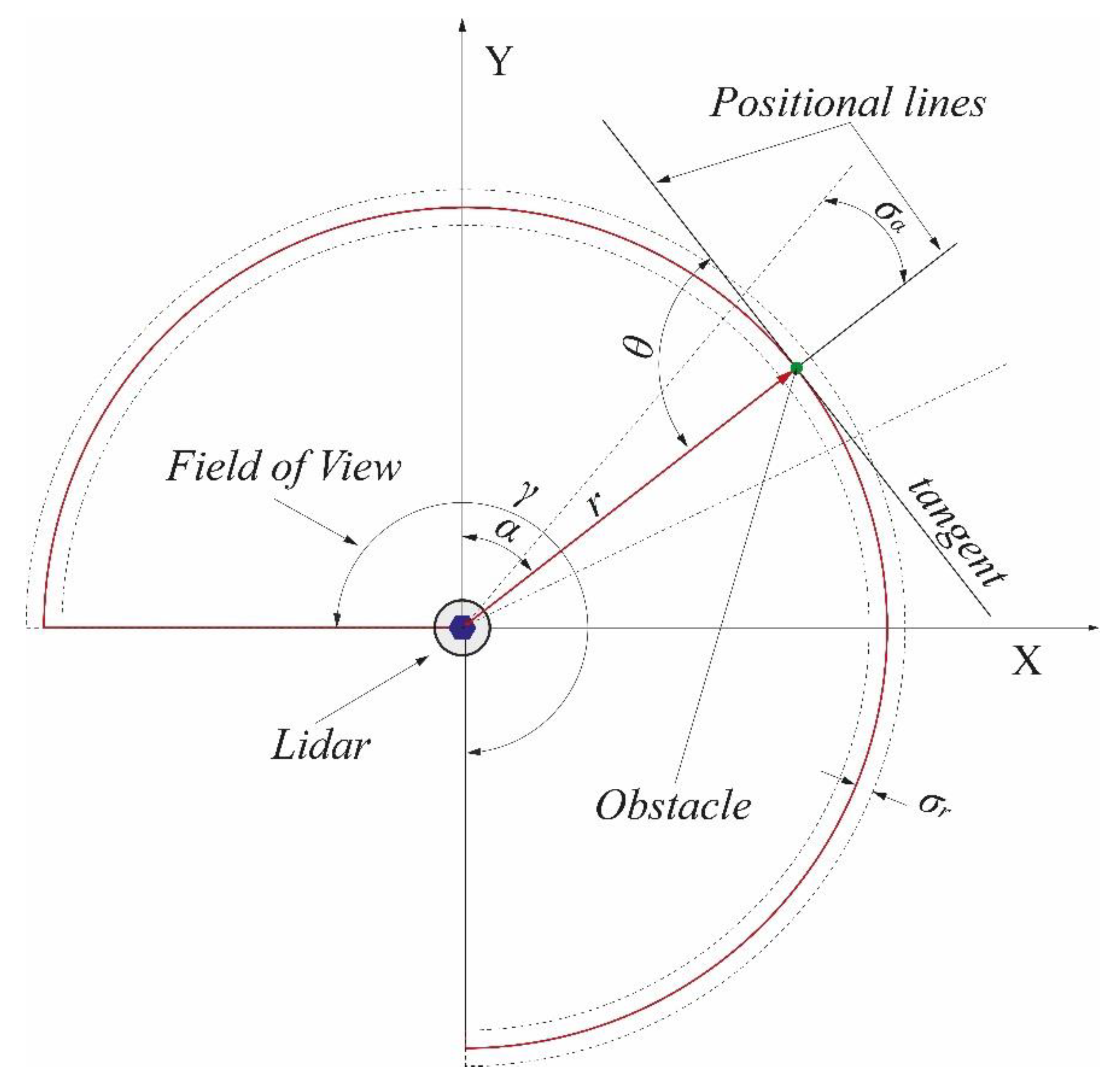
2. Evaluation of the Accuracy of Determining the Coordinates of a Position Using LIDAR

The determination of horizontal coordinates using LIDAR is carried out based on the angle $\alpha$ and the distance $r$ measured between the sensor and the target, i.e., the light signal reflection point (Figure 1).

The mean error M and the parameters of mean error ellipse (i.e., the lengths of semi-axes $a$ and $b$) of the determination of 2D horizontal coordinates $\left(\mathrm{x},\mathrm{y}\right)$ using LIDAR can be calculated by applying the law of mean error propagation [35,36]. When the functions of a single result of the following measurement are known:

$$\alpha =\mathrm{arc}\mathrm{tg}\frac{x}{y},$$

(1)

$$r=\sqrt{x^2+y^2},$$

(2)

equations of the mean errors of positional lines can be written as:

$${\sigma }_{l(\alpha )}={\sigma }_{\alpha }/\sqrt{{\left(\frac{\partial \alpha }{\partial x}\right)}^2+{\left(\frac{\partial \alpha }{\partial y}\right)}^2},$$

(3)

$${\sigma }_{l\left(r\right)}={\sigma }_r/\sqrt{{\left(\frac{\partial r}{\partial x}\right)}^2+{\left(\frac{\partial r}{\partial y}\right)}^2},$$

(4)

which enable the determination of mean error of position:

$$M=\frac{1}{\sin \theta }\sqrt{{{\sigma }_{l(\alpha )}}^2+{\sigma }_{l\left(r\right)}{}^2}=\sqrt{{\left({\sigma }_{\alpha }·r\right)}^2+{\sigma }_r{}^2},$$

(5)

$$a={\sigma }_{\alpha }·r,$$

(6)

$$b={\sigma }_r,$$

(7)

where: $\theta$—the angle of intersection of positional lines, which for LIDAR measurements is always equal to 90°,

σ_α—mean error of the angle measurement α,

${\sigma }_r$—mean error of the distance measurement $r$,

$r$—distance between the sensor and the target,

$a$—the length of the long semi-axis of mean error ellipse (see Figure 2),

$b$—the length of the short semi-axis of mean error ellipse (see Figure 2).

It follows from Dependence (5) that the value of mean error $\mathrm{M}$ and the length of the long semi-axis $\mathrm{a}$ of the mean error ellipse are significantly affected by the distance $\mathrm{r}$ between the sensor and the target. The calculations assumed that the measurements were performed using the Scanse Sweep LIDAR [37] for which the manufacturer provides ${\sigma }_r=0.004258·r$ (rounded value). Thereby one takes into account the fact that the error value of the angle measurement does not only depend on the beam’s divergence (footprint of the beam increases as a function of divergence) and the angle of its incidence on the surface of the object, but also on the accuracy of measuring the angle change by the optical head encoder that can be affected by environmental conditions such as temperature and humidity, vibrations and imperfections in the performance of mechanical elements that cooperate with each other. This can be characteristic for entry level LIDAR devices. The spatial angle resolution can be derived from sampling frequency that is set up to 1000 Hz (when optical sensor is spinning with frequency 1 Hz the Lidar is able to sample up to 1000 point for a single spin, 5 Hz—200 points, 10 Hz—100 points). The range spatial resolution is around 0.1 cm.

Based on the known lengths of semi-axes $a$ and $b$ of the mean error ellipse, and based on the known direction of α measurement, one can simply generate a covariance matrix $cov$ of the $\left(\mathrm{x},\mathrm{y}\right)$ vector coordinates:

$$cov\left(x, y\right)=\left[\begin{array}{cc} a^2·{\cos }^2{\alpha }_a+b^2·{\sin }^2{\alpha }_a& \left(a^2-b^2\right)·\sin {\alpha }_a·\cos {\alpha }_a\\ \left(a^2-b^2\right)·\sin {\alpha }_a·\cos {\alpha }_a& a^2·{\sin }^2{\alpha }_a+b^2·{\cos }^2{\alpha }_a\end{array}\right],$$

(8)

where ${\alpha }_a$—is the angle between the semi-axis $\mathrm{a}$ of the mean error ellipse and the axis $\mathrm{OY}$ (for LIDAR measurements, equal to $\alpha +90°$).

Then, using this, to determine the mean square error ${\sigma }_{\beta }{}^2$ of the determination of the position coordinates, but in the specified direction β:

$$\begin{array}{ll}{\sigma }_{\beta }{}^2=S_{\beta }·cov\left(x, y\right)·S_{\beta }^{\mathrm{T}}& =\sin \beta ·(\sin \beta \left(r^2·{\sigma }_{\alpha }{}^2·{\sin }^2{\alpha }_a+{\sigma }_r{}^2·\cos {\alpha }_a\right)-\\ & -\cos {\alpha }_a·\cos \beta ·\sin {\alpha }_a\left({\sigma }_r{}^2-r^2·{\sigma }_{\alpha }{}^2\right))+\\ & +\sin \beta ·(\sin \beta ·\left(r^2·{\sigma }_{\alpha }{}^2·{\cos }^2{\alpha }_a+{\sigma }_r{}^2·{\sin }^2{\alpha }_a\right)-\\ & -\cos {\alpha }_a·\sin {\alpha }_a·\sin \beta ·\left({\sigma }_r{}^2-r^2·{\sigma }_{\alpha }{}^2\right)),\end{array}$$

(9)

where $S_{\beta }=\left[\begin{array}{cc}\cos \beta & \sin \beta \end{array}\right].$

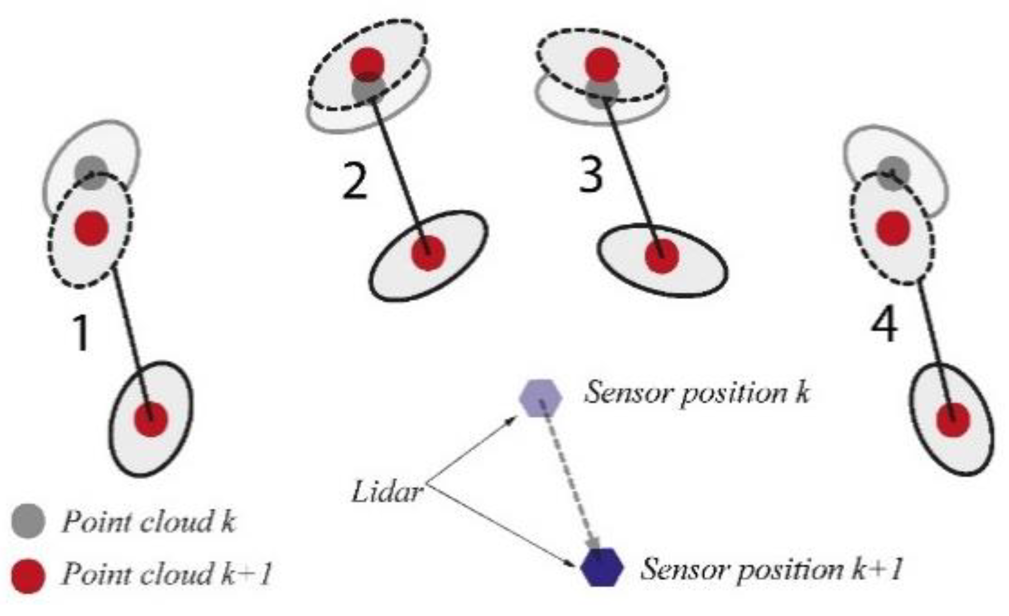
2.1. The Determination of USV Movement Parameters Using the Scan-Matching Method

The taxonomy of the ICP algorithm is carried out in the following successive stages of data processing [21]:

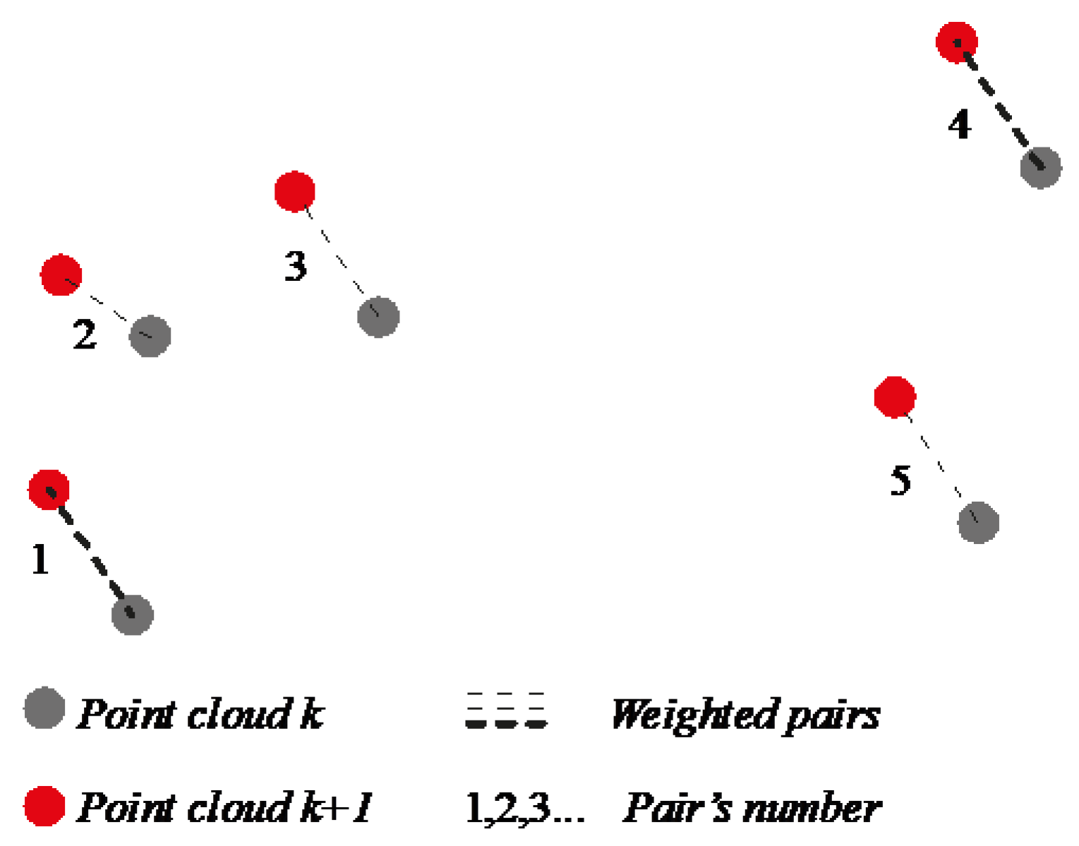
• Selection (selection of points which are suitable for the alignment);
• Matching (matching points from model cloud to reference points cloud);
• Weighting (giving weight to corresponding points);
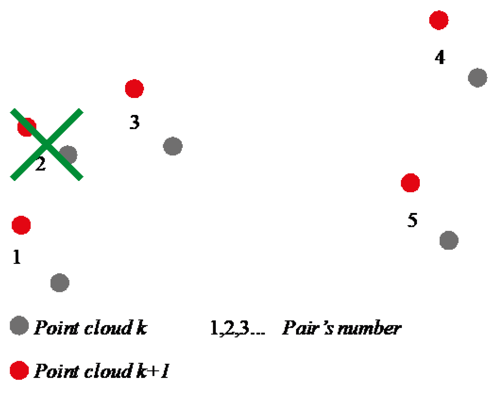
• Rejecting (deleting some points based on the robust criterion function);
• Assigning an error metric (choosing point-to-point, point-to-line, point-to-plane or plane-to-plane error metric);
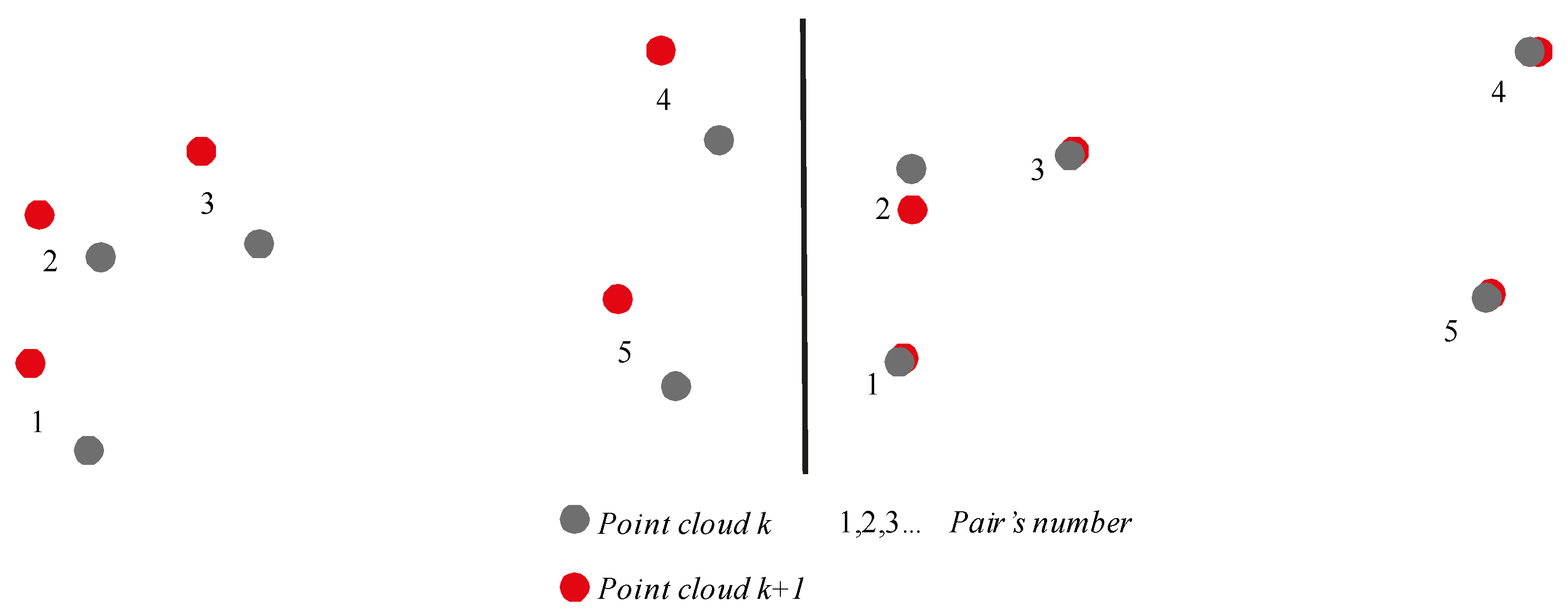
• Minimizing the metric between selected points.

Selection. Let us assume that a USV determines the change in its position through the translation vector $T\left(k+1\right)$ and the rotation matrix $R\left(k+1\right)$ determined based on two maps of the surrounding environment $M\left(k\right)$ and $M\left(k+1\right)$, constructed at the moment $\left(k\right)$ and the moment $\left(k+1\right)$ following it (e.g., 2D horizontal layer of cloud points for LIDAR measurements). Let $\mathbb{Z}\left(k\right)$ and $\mathbb{Z}\left(k+1\right)$ represent two sets $\left\{\left(r_1\left(k\right),{\alpha }_1\left(k\right)\right), \dots ,\left(r_n\left(k\right),{\alpha }_n\left(k\right)\right)\right\}$ and $\left\{\left(r_1\left(k+1\right),{\alpha }_1\left(k+1\right)\right), \dots ,\left(r_n\left(k+1\right),{\alpha }_n\left(k+1\right)\right)\right\}$ of measurements of the distance r and direction α, carried out in relation to $n$ field obstacles (see Figure 1). On their basis, set of points $M\left(k\right)=\left\{p_1\left(k\right), \dots ,p_{\mathrm{n}}\left(k\right)\right\}$ and $M\left(k+1\right)$ = $\left\{p_1\left(k+1\right), \dots ,p_{\mathrm{n}}\left(k+1\right)\right\}$ will be determined, where the coordinates of each point in the formula are calculated via the following dependence:

$$\begin{array}{r}{p}_{\mathrm{i}}=\left[\begin{array}{c}{x}_i\\ y_i\end{array}\right],\\ x_i=r_i·\cos \left({\alpha }_i\right),\\ y_i=r_i·\sin \left({\alpha }_i\right),\end{array}$$

(10)

where:

$$i=1,\dots ,n$$

They will be used to determine the translation vector $T\left(k+1\right)$ and the rotation matrix $R\left(k+1\right)$ using the singular value decomposition (SVD) method [38], which will be carried out in combination with a change in the position (in subsequent iteration steps) of the set of points from $M\left(k\right)$ to $M\left(k+1\right)$ using the modified weighted ICP method. In reality, there is very little probability that both sets of points $M\left(k\right)$ and $M\left(k+1\right)$ will contain the same number of points. Equalising the number of points is required for the family of ICP algorithms with point-to-point error metric and therefore, in the calculations they were carried out by reducing the number of points. From a more numerous set, the points were randomly removed so that their number would be equal to the number of the points from a smaller set.

Matching. Literature shows that there are many ways to match points in pairs. One of them is the k-d tree method presented in [39,40]. Also considered are methods based on the heuristic search of pairs to reduce the complexity of calculations [41]. In this article, correspondence between points is created based on the method presented in [42]. It is based on the Delaunay triangulation. The method generates a two-dimensional grid of triangles based on the reference set $M\left(k\right)$. Next, using the nearest neighbor method, the nearest apex of triangles to the points from the set $M\left(k+1\right)$ are found (points from $M\left(k\right)$) in such a way that for each point $p_i\left(k\right)$ the nearest point $p_{id\left(i\right)}\left(k+1\right)\mathrm{is}\mathrm{assigned}$ (see Figure 3).

Weighting of the pairs. The modification of the ICP method will involve the application of the weighting factor $w_{1,\dots ,n}\left(k,k+1\right)$ for calculations for each pair of points (nearest neighbors):

$$w_{\mathrm{i}}\left(k,k+1\right)=\frac{1}{\sqrt{G_{\mathrm{i}}\left(k,k+1\right)}},$$

(11)

where $G_i\left(k, k+1\right)$ is the sum of mean errors of the determination of the coordinates of points $p_i\left(k\right)$ and $p_{id\left(i\right)}\left(k+1\right)$ in the specified direction $\beta$ (see Figure 2):

$$G_i\left(k,k+1\right)={\sigma }_{\beta }{}_i^2\left(k\right)+{\sigma }_{\beta }{}_{id\left(i\right)}^2\left(k+1\right),$$

(12)

where ${\sigma }_{\beta }{}_i\left(k\right)$ is the mean error of the determination of the coordinates of the point $p_i\left(k\right)$ in the direction of $\beta$ (from $p_i\left(k\right)$ to $p_{id\left(i\right)}\left(k+1\right))$, ${\sigma }_{\beta }{}_{id\left(i\right)}\left(k+1\right)$ is the mean error of the determination of the coordinates of the point $p_i\left(k+1\right)$ in the direction of $\beta$ (from $p_{id\left(i\right)}\left(k+1\right)$ to $p_i\left(k\right))$, or $G_i\left(k, k+1\right)$ is the mean error of the determination of the coordinates of the points $p_i\left(k\right)$ and $p_{id\left(i\right)}\left(k+1\right)$ (see Figure 1):

$$G_i\left(k,k+1\right)=M_i^2\left(k\right)+M_{id\left(i\right)}^2\left(k+1\right),$$

(13)

where $M_i\left(k\right)$ is the mean error of the determination of the coordinates of the point $p_i\left(k\right)$, $M_{id\left(i\right)}\left(k+1\right)$ is the mean error of the determination of the coordinates of the point $p_{id\left(i\right)}\left(k+1\right)$.

Weighting step gives specific calculated value for each pair. Then in further processing heavier pairs involve more the translation and rotation parameters (Figure 4).

Rejection. Due to the relatively high noise level of many scans, particularly in the sectors illustrating long distance measurements, the Huber function [43] which attenuated the outlying measurement results (affected by gross errors) was also applied in the calculations. This function was arbitrarily selected from among many functions known and commonly used for this purpose [21,31,44,45,46,47]. The robust function rejects or significantly reduces weights of the specific pairs due to robustness criterion (see Figure 5). The robust function is based on $kHu$ factor presented in Algorithm 1. Rejecting or weight minimization is performed based on norm of two paired points. In this article the fusion of the robust function and proposed error weighting is used to derivate the final weight.

Assigning an error metric. The final function minimizing the value of the matching error $\mathrm{E}$, used to accurately determine the translation vector $T\left(k+1\right)$ and the rotation matrix $R\left(k+1\right)$, will take the following form:

$$\mathrm{E}\left(R, T\right)= {{\displaystyle \sum }}_{i=1}^n{w}_i\left(k,k+1\right)·\Vert R{p}_i\left(k\right)+T-p_{id\left(i\right)}\left(k+1\right){\Vert }^2.$$

(14)

Provided that points $p_i\left(k\right)$ and $p_{id\left(i\right)}\left(k+1\right)$ are located the closest to one another, i.e., are the nearest neighbors. This method is based on the point-to-point measure of error.

Minimizing the metric between selected points. The method of minimizing the error between the corresponding points was carried out on the basis of the SVD (Singular Value Decomposition). The method works equally for the weighted and classical ICP algorithm. In this article a method identical to [47] was used. It is required to determine two weighted average coordinates from the cloud $\mathrm{m}\left(k\right)$ and $\mathrm{m}\left(k+1\right)$, dependent on point clouds $\left(k\right),\left(k+1\right)$ and assigned weights in the previous stage:

$$\mathrm{m}\left(k\right)=\frac{{{\displaystyle \sum }}_{i=1}^n{w}_i·{\mathrm{p}}_i\left(k\right)}{{{\displaystyle \sum }}_{i=1}^n{w}_i},$$

(15)

$$\mathrm{m}\left(k+1\right)=\frac{{{\displaystyle \sum }}_{i=1}^n{w}_{id\left(i\right)}·{\mathrm{p}}_{id\left(i\right)}\left(k+1\right)}{{{\displaystyle \sum }}_{i=1}^n{w}_i}.$$

(16)

Subsequently, we can move on to determine the weighted covariance matrix, which will be used to calculate the innovation of rotation matrix and translation (in a given iteration of the algorithm)

$$C=\frac{{{\displaystyle \sum }}_{i=1}^n\left(w_i·p_i\left(k\right)·p_{\mathrm{id}\left(\mathrm{i}\right)}^{\mathrm{T}}\left(k+1\right)\right)}{{{\displaystyle \sum }}_{i=1}^n{w}_i}-\mathrm{m}\left(k\right)·{\mathrm{m}}^{\mathrm{T}}\left(k+1\right).$$

(17)

Using the SVD decomposition method on the C matrix

$$C=U\Sigma V^T.$$

(18)

where matrices U, Σ, V are characteristic matrices for the SVD method. By means of decomposition carried out on designated matrices, we obtain the innovations in given iteration—$it$—of the ${\mathrm{R}}_{it}$ rotation matrix and the $T_{it}$ translation:

$$R_{it}=V{U}^{\mathrm{T}},$$

(19)

$$T_{it}=\mathrm{m}\left(k\right)-R_{it}·\mathrm{m}\left(k+1\right).$$

(20)

The obtained values in the $R_{iter}$ and $T_{iter}$ matrices are partial values developed in a given iteration of the algorithm. Based on this, the set m(k + 1) is translated at last iteration (see Figure 6) and as a result the translation and rotation is obtained:

$$R\left(k+1\right)=R_1·\dots ·R_{itn},$$

(21)

$$T\left(k+1\right)=(R_{it+1}·T_{it}+T_{it+1})+\dots +(R_{\mathrm{itn}}·T_{\mathrm{itn}-1}+T_{\mathrm{itn}}).$$

(22)

where $R_{it=1}$ and $T_{it=1}$ are initialized values.

The translation vector $T\left(k+1\right)=\left[\begin{array}{c}\Delta x\\ \Delta y\end{array}\right]$ thus obtained will be used to determine

$$\mathrm{SOG}\left(k+1\right)=\frac{\sqrt{\Delta x^2+\Delta y^2}}{\Delta t},$$

(23)

where $\Delta t$ is the distance in time between the moment $\left(k\right)$ of performing the measurements of $\mathbb{Z}\left(k\right)$, and the moment $\left(k+1\right)$ of performing subsequent measurements of $\mathbb{Z}\left(k+1\right)$.

On the other hand, the final form of the rotation matrix $R\left(k+1\right)=\left[\begin{array}{cc}\cos \Delta \theta & \sin \Delta \theta \\ -\sin \Delta \theta & \cos \Delta \theta \end{array}\right]$ will be used to determine:

$$\mathrm{ROT}\left(k+1\right)=\frac{\mathrm{arc}\sin \left(\Delta \theta \right)}{\Delta t},$$

(24)

and

$$\mathrm{HDG}\left(k+1\right)={\mathrm{HDG}}_0+\mathrm{arc}\sin \left(\Delta \theta \right),$$

(25)

where ${\mathrm{HDG}}_0$ is the initial HDG value determined using other methods (devices) prior to the commencement of measurement.

2.2. Weighted Matching Point Clouds Using the Mean Direction Error

Figure 7 shows that the mean error value changes significantly as the function of angle $\beta$, and the gradient of these changes will increase while the eccentricity of the ellipse is approaching 1 (the ellipse will be becoming flat, which occurs where measurements are carried out using LIDAR). Owing to these particular properties, this error can usefully determine the value of translation and rotation established while minimalizing the error metric between the points from subsequent measurements (e.g., point clouds from LIDAR measurements). Figure 8 presents, in the graphical form, how the positions matched in pairs of points based on the corrections (e.g., those added to the components of the rotation matrix and translation vector) change; the value of the rotation and translation was made depending on the values of the sums of mean errors (Equation (9)) calculated along lines connecting the matched points from $\left(k\right)$ and $\left(k+1\right)$ cloud. In order to facilitate the interpretation of the phenomenon, it was assumed that the mean error ellipses were similar in size.

As can be seen in Figure 7, greater weight is introduced for the points whose mean errors in the specified direction (point-to-point direction) is lower–pairs marked as 2 and 3 in Figure 7. The heavier weight influences the rotation and translation more and that is why pair 2 and 3 are better aligned comparing with 1 and 4. The use of such a weighting coefficient allows taking into account the spatial distribution of errors according to the selected direction. For comparison, Figure 8 presents, in a graphical form, how the positions matched in pairs of points based on the corrections whose values depended on the values of the sums of mean errors (Equation (5)) calculated for the matched points. As can be seen each pair (1, 2, 3, 4) influences the rotation and translation in similar manner.

HDG, SOG, and ROT were determined by processing LIDAR scans archived in data packets in accordance with the methodology presented in Section 2.1. The pseudo-code of the program used for the calculations using the authors original weighting factor $w\left(k,k+1\right)$ and Huber’s robust function coefficient $kHu=c·\mathrm{Median}\Vert p_{1,\dots ,n}\left(k\right)-p_{id\left(1,\dots n\right)}\left(k+1\right)\Vert$ finally took the following form:

Algorithm 1 The weighted ICP

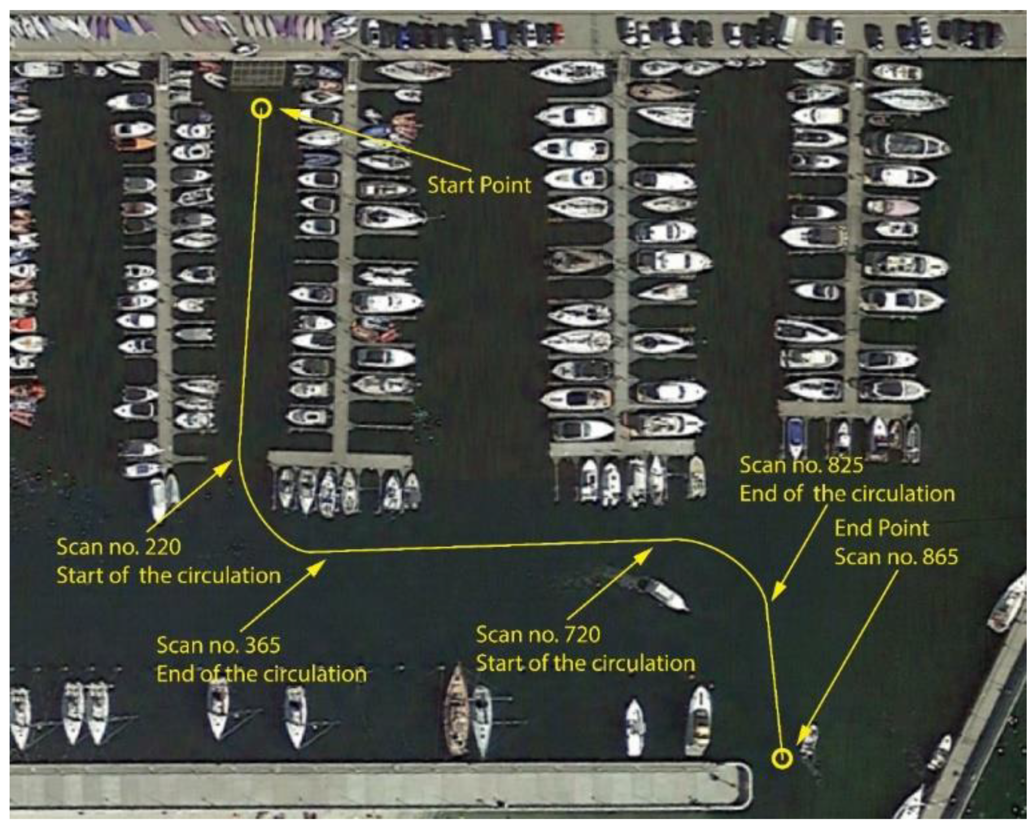
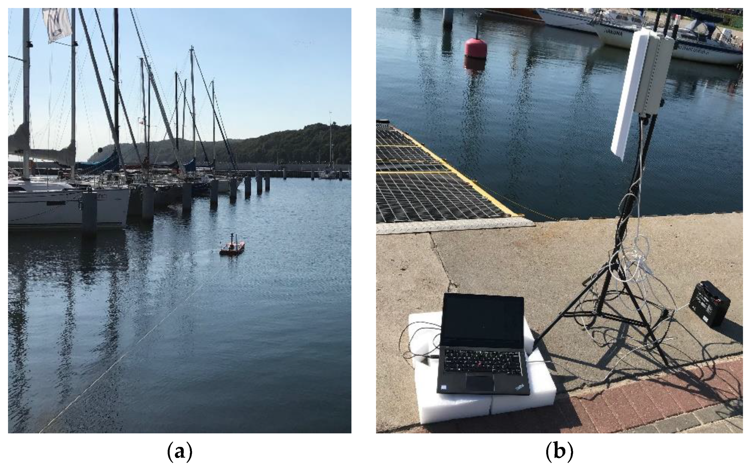
3. The Study and the Analysis of the Obtained Results

The main aim of the study was to evaluate the accuracy of the determination of the HDG, SOG and ROT using a modified ICP algorithm, carried out as a result of their comparison with high-accuracy reference measurements. The study involved:

• measurements carried out using LIDAR and a GNSS RTK receiver, and the synchronous recording of their results,
• the determination of the HDG, SOG and ROT, based on LIDAR measurement results, by the scan-matching method using both classic and modified versions of the ICP algorithm,
• an analysis comparing the HDG, SOG, and ROT with reference results of GNSS RTK measurements, based on the accuracy criterion.

The yacht port basin in Gdynia (Poland) was selected for the measurement area. Its boundaries include high, concrete wharves and a breakwater. Most of the time, good hydro-meteorological conditions prevail in the area (Figure 9). To carry out the measurements, a small USV (with a length of 1.62 m, width of 0.40 m, and a draught of 0.11 m) equipped with Scanse Sweep Lidar, a GNSS RTK receiver Leica Viva CS 15 [48], and an on-board computer connected to them with a RS-422/232C conversion cable [49], were used to record the measurement results (Figure 10). The measurements were carried out on a USV sailing with a speed of approximately $1.2\frac{\mathrm{m}}{\mathrm{s}}\left(2.4\mathrm{kts}\right)$ over a trajectory of approximately $220 \mathrm{m}$, as presented in Figure 10. All data was collected via a mobile computer wirelessly connected to AUSV (autonomous unmanned surface vehicle, see Figure 11.). While the USV was sailing, the on-board computer synchronously recorded (when generating a full scan using LIDAR) the measurement results making up the so-called data sets containing: a LIDAR scan (in the form of a measurement set $\mathbb{Z}=\left\{\left(r_1,{\alpha }_1\right), \dots ,\left(r_{\mathrm{n}},{\alpha }_{\mathrm{n}}\right)\right\}$), NMEA messages with the position coordinates of SOG and COG (course over ground) from the GNSS RTK receiver [50]. 865 data sets were thus collected by recording each subsequent sets every $0.2 \mathrm{s}$ on average, i.e., after a change in the USV position by approx. $0.25 \mathrm{m}$.

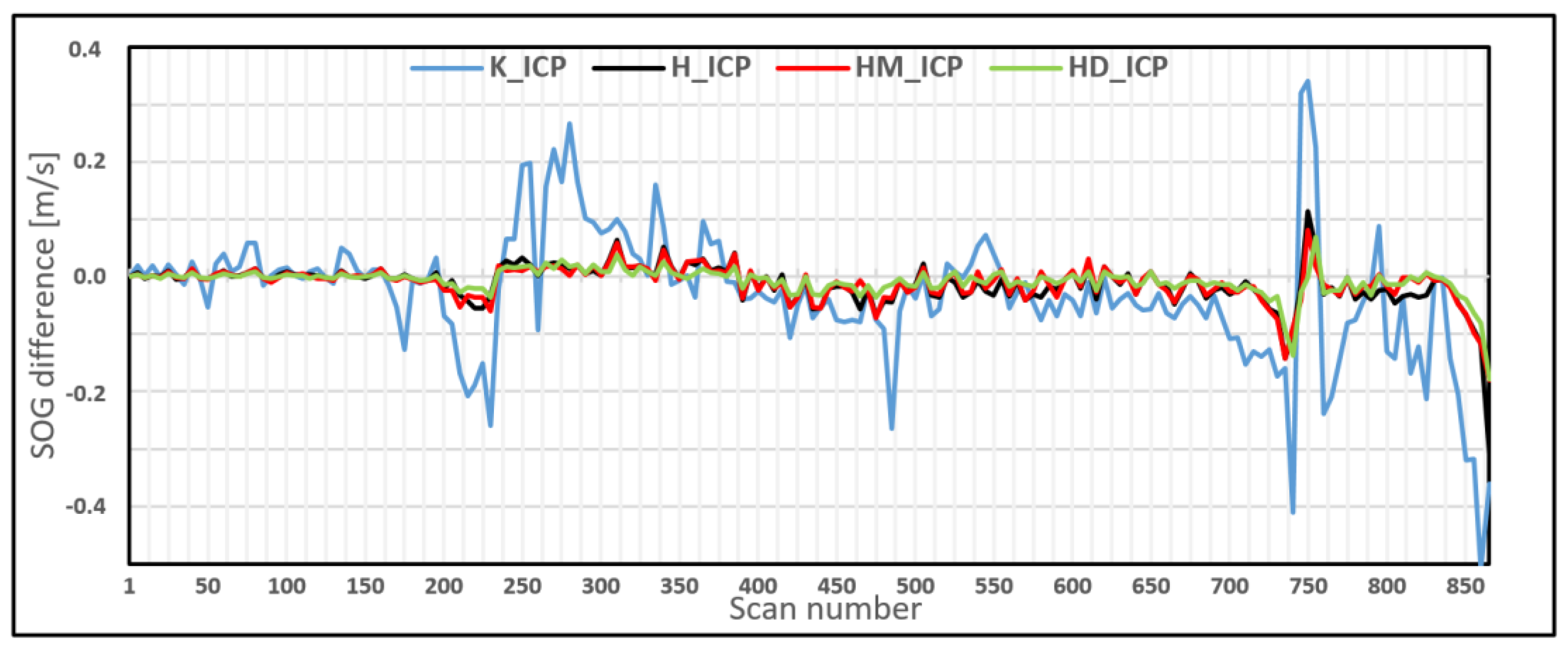
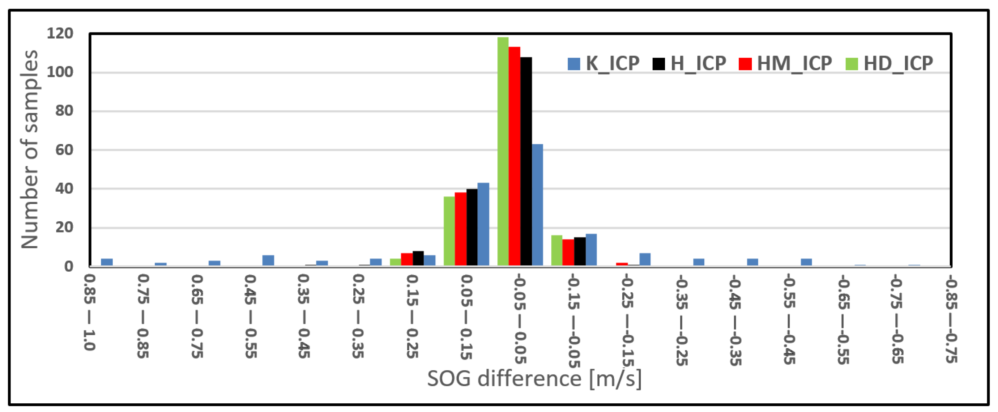
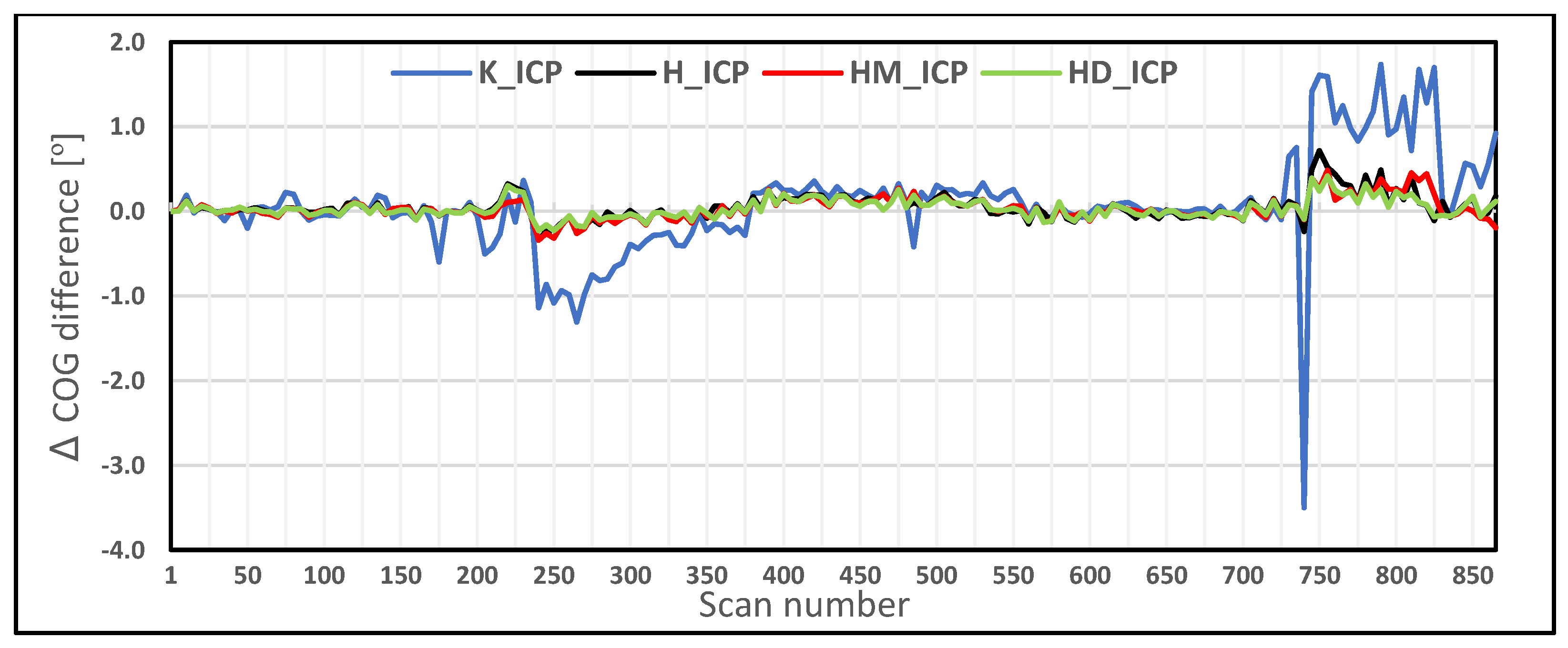
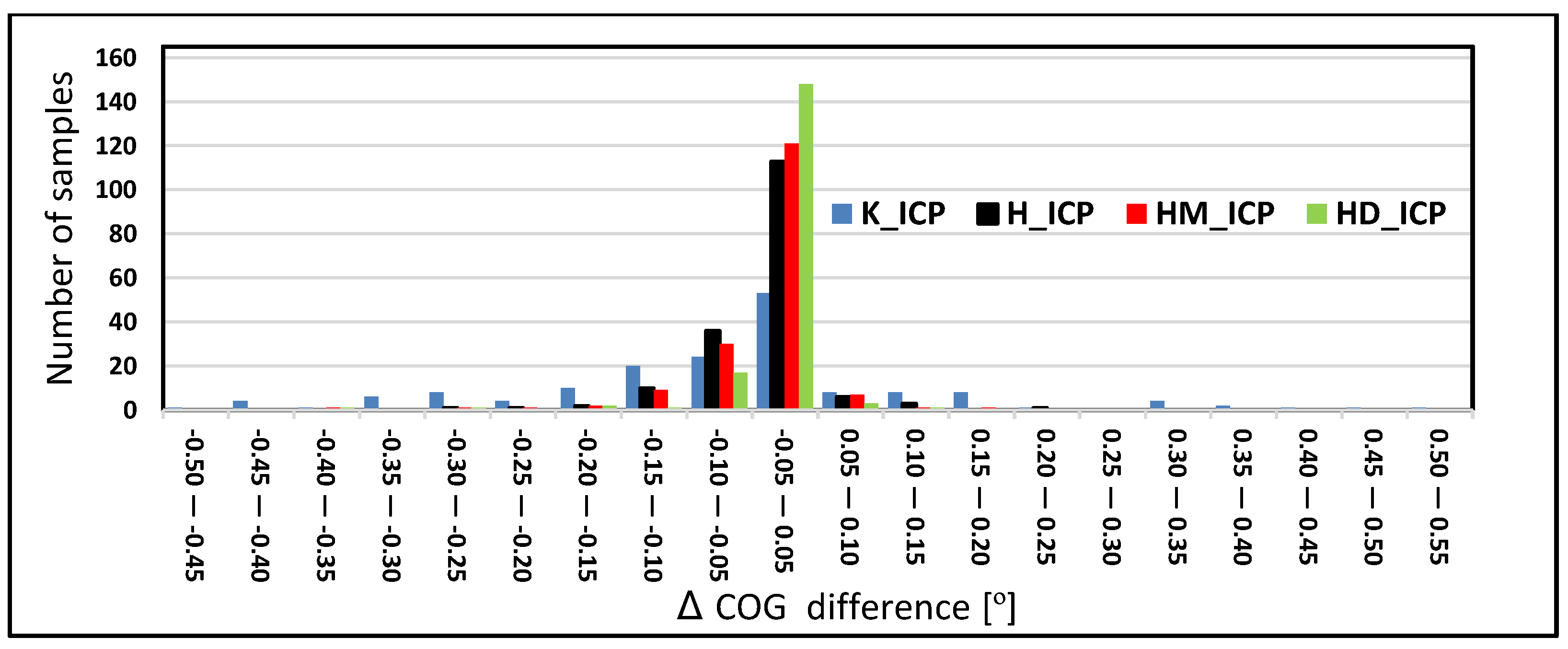
Analysis of the Accuracy of Determining the COG and SOG Using a Modified ICP Algorithm

Table 1. Summary of comparative statistical parameters.

Method	Mean Value		Standard Deviation		Maximum Value
	$\mathbf{S}\mathbf{O}{\mathbf{G}}_{\mathbf{I}\mathbf{C}\mathbf{P}}-\mathbf{S}\mathbf{O}{\mathbf{G}}_{\mathbf{R}}$$\left(\mathbf{m}/\mathbf{s}\right)$	$\mathsf{\Delta }\mathbf{C}\mathbf{O}{\mathbf{G}}_{\mathbf{I}\mathbf{C}\mathbf{P}}-\mathsf{\Delta }\mathbf{C}\mathbf{O}{\mathbf{G}}_{\mathbf{R}}$$(°)$	$\mathbf{S}\mathbf{O}{\mathbf{G}}_{\mathbf{I}\mathbf{C}\mathbf{P}}-\mathbf{S}\mathbf{O}{\mathbf{G}}_{\mathbf{R}}$$\left(\mathbf{m}/\mathbf{s}\right)$	$\mathsf{\Delta }\mathbf{C}\mathbf{O}{\mathbf{G}}_{\mathbf{I}\mathbf{C}\mathbf{P}}-\mathsf{\Delta }\mathbf{C}\mathbf{O}{\mathbf{G}}_{\mathbf{R}}$$(°)$	$\mathbf{S}\mathbf{O}{\mathbf{G}}_{\mathbf{I}\mathbf{C}\mathbf{P}}-\mathbf{S}\mathbf{O}{\mathbf{G}}_{\mathbf{R}}$$\left(\mathbf{m}/\mathbf{s}\right)$	$\mathsf{\Delta }\mathbf{C}\mathbf{O}{\mathbf{G}}_{\mathbf{I}\mathbf{C}\mathbf{P}}-\mathsf{\Delta }\mathbf{C}\mathbf{O}{\mathbf{G}}_{\mathbf{R}}$$(°)$
K_ICP	−0.031	0.08	0.113	0.57	−0.524	−3.5
H_ICP	−0.013	0.05	0.031	0.14	−0.319	0.72
HM_ICP	−0.012	0.03	0.031	0.13	−0.185	−0.48
HD_ICP	−0.007	0.03	0.026	0.11	−0.18	0.42

presents statistical parameters (i.e., the mean value, standard deviation and the maximum value) which characterize the computational accuracy of each parameter. The following acronyms were used to describe ICP’s variants: K_ICP for algorithm without modification, H_ICP for robust version based on Huber’s function, HM_ICP for robust version based on Huber’s function with mean error weighting and HD_ICP for robust version based on Huber’s function with directional error weighting. The lower index ICP was used for values computed by ICP algorithm’s variants and lower index R was introduced to point the values surveyed with GNSS RTK receiver.

A comparison of the parameter values (obtained based on 865 collected data packets) listed in Table 1 shows that the HD_ICP algorithm was the best in terms of the accuracy of determining the USVs movement parameters; it is followed by HM_ICP, H_ICP and K_ICP. Figure 12 shows a graph of SOG_ICP-SOG_R differences.

Figure 12 shows that the accuracy of determining the SOG using the K_ICP method significantly decreases for scans in the intervals of $\langle 220, 365\rangle$ and $\langle 720, 825\rangle$. These scans differ significantly from each other in rotation angles and include a greater number of erroneous measurement results than the others. This is undoubtedly due to the turns made by the USV at that time. The accuracy of determining the SOG using the other methods is, at the same time, considerably higher. These methods probably achieve that through the attenuation of measurements with gross errors using Huber’s function. The HD_ICP method proved to be the best in determining the SOG in a significant part of the graph course. This was also confirmed by the lowest values of the mean error, equal to $-0.007\frac{\mathrm{m}}{\mathrm{s}}\left(-0.014 \mathrm{kts}\right)$ and of the standard deviation, equal to $0.026 \frac{\mathrm{m}}{\mathrm{s}} \left(0.05 \mathrm{kts}\right)$ presented in Table 1.

The histogram representing the frequency of occurrence of ${\mathrm{SOG}}_{\mathrm{ICP}}-{\mathrm{SOG}}_{\mathrm{R}}$ differences, presented in Figure 13, shows even more clearly that in terms of the accuracy of determining the SOG, the HD_ICP method is better than the others. Most of the values of ${\mathrm{SOG}}_{\mathrm{ICP}}-{\mathrm{SOG}}_{\mathrm{R}}$ differences, determined using the HD_ICP, HM_ICP, and H_ICP methods, fall within the interval of −0.05~0.05.

Figure 14 shows that the accuracy of determination of the $\mathsf{\Delta }\mathrm{COG}$ using the K_ICP method significantly decreases, as in the case of the SOG, for scans in the intervals of $\langle 220, 365\rangle$ and $\langle 720, 825\rangle$. The HD_ICP method also proved to be the best in determining the $\mathsf{\Delta }\mathrm{COG}$ in this case. This was also confirmed by the lowest values of the mean error, equal to $0.03°$, and of the standard deviation, equal to $0.11°$, presented in Table 1. Figure 15 shows a histogram representing the frequency of occurrence of ${\mathsf{\Delta }\mathrm{COG}}_{\mathrm{ICP}}-{\mathsf{\Delta }\mathrm{COG}}_{\mathrm{R}}$ increment differences.

The histogram representing the frequency of the occurrence of differences ${\mathsf{\Delta }\mathrm{COG}}_{\mathrm{ICP}}-{\mathsf{\Delta }\mathrm{COG}}_{\mathrm{R}}$ shown in Figure 15 enables the conclusion that the HD_ICP method is also the best in terms of the accuracy of determining the $\mathsf{\Delta }\mathrm{COG}$. Its advantage over the others can be clearly seen in the interval of differences ${\mathsf{\Delta }\mathrm{COG}}_{\mathrm{ICP}}-{\mathsf{\Delta }\mathrm{COG}}_{\mathrm{R}}$ $\langle -0.05˚, 0.05˚\rangle$. Given that the $\mathsf{\Delta }\mathrm{ROT}$ results are identical with the $\mathsf{\Delta }\mathrm{COG}$ results, their presentation and analysis have been omitted. Differences in the algorithms’ accuracy are shown at Figure 16 (presenting results of H_ICP and HD_ICP). Differences between HD_ICP and HM_ICP versions are barely visible, so they were omitted.

4. Conclusions

As the study attempted to prove, an ICP algorithm that matches point clouds from a laser scanner can effectively generate USV movement parameters. The proposed weighting factor based on the mean error in the specified direction of the determination of the coordinates of the positions of scan points enables more realistic (corresponding to the actual movement) matching of subsequent maps of the surrounding environment. This helps to determine the USV movement parameters with a higher accuracy. This was confirmed by the study results—inter alia the values of statistical indices in the form of mean ${\mathrm{SOG}}_{\mathrm{ICP}}-{\mathrm{SOG}}_{\mathrm{R}}=0.007 \frac{\mathrm{m}}{\mathrm{s}} \left(-0.014 \mathrm{kts}\right)$ and standard deviation ${\mathrm{SOG}}_{\mathrm{ICP}}-{\mathrm{SOG}}_{\mathrm{R}}=0.0025 \frac{\mathrm{m}}{\mathrm{s}} \left(0.05 \mathrm{kts}\right)$ and ${\mathsf{\Delta }\mathrm{COG}}_{\mathrm{ICP}}-{\mathsf{\Delta }\mathrm{COG}}_{\mathrm{R}}=0.03°$ and standard deviation ${\mathsf{\Delta }\mathrm{COG}}_{\mathrm{ICP}}-{\mathsf{\Delta }\mathrm{COG}}_{\mathrm{R}}=0.11°$. However, it should be noted that the authors’ original weighting factor should be used in combination with a robust criterion function to reduce measurements with gross errors (e.g., based on Huber’s function), as only such a solution can be fully applicable. The indicated mean error values lead us to a generalized statement that the developed method allows measuring SOG and COG with the accuracy required by the IMO. It should be noted, however, that the test was carried out in confined waters (harbors, channels, berths, marinas), beyond which the method would not be effective due to the low LIDAR range. All data used in publication is available at [51].

References

- IMO. Resolution A.824(19) Adoption of Amendments to Performance Standards for Devices to Measure and Indicate Speed and Distance; IMO: London, UK, 2000. [Google Scholar]
- IMO. Resolution MSC.116(73), Performance Standards for Marine Transmitting Heading Devices (thds); IMO: London, UK, 2000. [Google Scholar]
- Naus, K.; Waz, M. Precision in Determining Ship Position using the Method of Comparing an Omnidirectional Map to a Visual Shoreline Image. J. Navig. 2016, 69, 391–413. [Google Scholar] [CrossRef]
- Polvara, R.; Sharma, S.; Wan, J.; Manning, A.; Sutton, R. Obstacle Avoidance Approaches for Autonomous Navigation of Unmanned Surface Vehicles. J. Navig. 2018, 71, 241–256. [Google Scholar] [CrossRef]
- Allen, C.H. The Seabots are Coming Here: Should they be Treated as ‘Vessels’? J. Navig. 2012, 65, 749–752. [Google Scholar] [CrossRef]
- Nowak, A. The Proposal to “Snapshot” Raim Method for Gnss Vessel Receivers Working in Poor Space Segment Geometry. Pol. Marit. Res. 2015, 22, 3–8. [Google Scholar] [CrossRef]
- Xie, P.; Petovello, M.G. Measuring GNSS Multipath Distributions in Urban Canyon Environments. IEEE Trans. Instrum. Meas. 2015, 64, 366–377. [Google Scholar]
- Wang, Y.; Chen, X.; Liu, P. Statistical Multipath Model Based on Experimental GNSS Data in Static Urban Canyon Environment. Sensors 2018, 18, 1149. [Google Scholar] [CrossRef]
- Shafiee, E.; Mosavi, M.R.; Moazedi, M. Detection of Spoofing Attack using Machine Learning based on Multi-Layer Neural Network in Single-Frequency GPS Receivers. J. Navig. 2018, 71, 169–188. [Google Scholar] [CrossRef]
- Guo, R.; Sun, F.; Yuan, J. ICP based on Polar Point Matching with application to Graph-SLAM. In Proceedings of the 2009 International Conference on Mechatronics and Automation, Changchun, China, 9–12 August 2009; pp. 1122–1127. [Google Scholar]
- Navarro, W.; Vélez, J.C.; Orfila, A. Estimation of sea state parameters using X-band marine radar technology in coastal areas. In Proceedings of the Sixth International Conference on Remote Sensing and Geoinformation of the Environment (RSCy2018), Paphos, Cyprus, 26–29 March 2018. [Google Scholar]
- Mendes, E.; Koch, P.; Lacroix, S. ICP-based pose-graph SLAM. In Proceedings of the 2016 IEEE International Symposium on Safety, Security, and Rescue Robotics (SSRR), Lausanne, Switzerland, 23–27 October 2016; pp. 195–200. [Google Scholar]
- Yang, J.; Li, H.; Jia, Y. Go-ICP: Solving 3D Registration Efficiently and Globally Optimally. In Proceedings of the 2013 IEEE International Conference on Computer Vision, Sydney, Australia, 1–8 December 2013; pp. 1457–1464. [Google Scholar]
- Zhang, Z. Iterative point matching for registration of free-form curves and surfaces. Int. J. Comput. Vis. 1994, 13, 119–152. [Google Scholar] [CrossRef]
- Men, H.; Gebre, B.; Pochiraju, K. Color point cloud registration with 4D ICP algorithm. In Proceedings of the 2011 IEEE International Conference on Robotics and Automation, Shanghai, China, 9–13 May 2011; pp. 1511–1516. [Google Scholar]
- Durrant-Whyte, H.; Bailey, T. Simultaneous localization and mapping: Part I. IEEE Robot. Autom. Mag. 2006, 13, 99–110. [Google Scholar] [CrossRef]
- Moratuwage, M.D.P.; Wijesoma, W.S.; Kalyan, B.; Dong, J.F.; Namal Senarathne, P.G.C.; Hover, F.S.; Patrikalakis, N.M. Collaborative multi-vehicle localization and mapping in marine environments. In Proceedings of the OCEANS’10 IEEE SYDNEY, Sydney, Australia, 24–27 May 2010; pp. 1–6. [Google Scholar]
- Ribas, D.; Ridao, P.; Neira, J. Underwater SLAM for Structured Environments Using an Imaging Sonar; Springer Tracts in Advanced Robotics Springer Berlin Heidelberg: Berlin/Heidelberg, Germany, 2010; ISBN 978-3-642-14039-6. [Google Scholar]
- Nieto, J.; Bailey, T.; Nebot, E. Recursive scan-matching SLAM. Robot. Auton. Syst. 2007, 55, 39–49. [Google Scholar] [CrossRef]
- Pomerleau, F.; Colas, F.; Siegwart, R.; Magnenat, S. Comparing ICP variants on real-world data sets: Open-source library and experimental protocol. Auton. Robot. 2013, 34, 133–148. [Google Scholar] [CrossRef]
- Rusinkiewicz, S.; Levoy, M. Efficient variants of the ICP algorithm. In Proceedings of the Third International Conference on 3-D Digital Imaging and Modeling, Quebec City, QC, Canada, 28 May–1 June 2001; pp. 145–152. [Google Scholar]
- Olson, E. Robust and Efficient Robotic Mapping. Ph.D. Thesis, Department of Electrical Engineering and Computer Science, MIT, Cambridge, MA, USA, 2008. [Google Scholar]
- Konecny, J.; Prauzek, M.; Kromer, P.; Musilek, P. Novel Point-to-Point Scan Matching Algorithm Based on Cross-Correlation. Mob. Inf. Syst. 2016, 2016, 1–11. [Google Scholar] [CrossRef]
- Besl, P.J.; McKay, N.D. A method for registration of 3-D shapes. IEEE Trans. Pattern Anal. Mach. Intell. 1992, 14, 239–256. [Google Scholar] [CrossRef]
- Callmer, J.; Törnqvist, D.; Gustafsson, F.; Svensson, H.; Carlbom, P. Radar SLAM using visual features. EURASIP J. Adv. Signal Process. 2011, 2011, 71–82. [Google Scholar] [CrossRef]
- Amigoni, F.; Gasparini, S.; Gimi, M. Scan matching without odometry information. In Proceedings of the First International Conference on Informatics in Control, Automation and Robotics, SciTePress—Science and Technology Publications, Setúbal, Portugal, 25–28 August 2004; pp. 349–352. [Google Scholar]
- He, Y.; Liang, B.; Yang, J.; Li, S.; He, J. An Iterative Closest Points Algorithm for Registration of 3D Laser Scanner Point Clouds with Geometric Features. Sensors 2017, 17, 1862. [Google Scholar] [CrossRef] [PubMed]
- Censi, A. An ICP variant using a point-to-line metric. In Proceedings of the 2008 IEEE International Conference on Robotics and Automation, Pasadena, CA, USA, 19–23 May 2008; pp. 19–25. [Google Scholar]
- Segal, A.; Haehnel, D.; Thrun, S. Generalized-ICP. In Proceedings of the Robotics: Science and Systems V; Robotics: Science and Systems Foundation, Boston, MA, USA, 28 June–01 July 2009. [Google Scholar]
- Wang, Y.; Xiong, R.; Li, Q. Em-based point to plane icp for 3d simultaneous localization and mapping. Int. J. Robot. Autom. 2013, 28. [Google Scholar] [CrossRef]
- Godin, G.; Rioux, M.; Baribeau, R. Three-Dimensional Registration Using Range and Intensity Information; The International Society for Optical Engineering: Boston, MA, USA, 1994. [Google Scholar]
- Marinov, A.; Zlateva, N.; Dimov, D.; Marinov, D. Weighted ICP Algorithm for Alignment of Stars from Scanned Astronomical Photographic Plates. Serdica J. Comput. Sofia Bulg. 2012, 6, 101–110. [Google Scholar]
- Amamra, A.; Aouf, N.; Stuart, D.; Richardson, M. A recursive robust filtering approach for 3D registration. SignalImage Video Process. 2016, 10, 835–842. [Google Scholar] [CrossRef]
- Wang, R.; Geng, Z. WA-ICP algorithm for tackling ambiguous correspondence. In Proceedings of the 2015 3rd IAPR Asian Conference on Pattern Recognition (ACPR), Kuala Lumpur, Malaysia, 3–6 November 2015; pp. 76–80. [Google Scholar]
- Naus, K.; Wąż, M. Ripping Radar Image with the Sea Map Using the Alignment Method 2009–2019; Logistyka, Institute of Logistics and Warehousing: Poznan, Poland, 2010. [Google Scholar]
- Naus, K.; Wąż, M. Accuracy in fixing ship’s positions by camera survey of bearings. Geod. Cartogr. 2011, 60, 61–73. [Google Scholar] [CrossRef]
- Scansce. User’s Manual and Technical Specifications. Available online: www.robotshop.com/ media/files/pdf2/sweep_user_manual.pdf (accessed on 1 February 2019).
- Marden, S.; Guivant, J. Improving the Performance of ICP for Real-Time Applications using an Approximate Nearest Neighbour Search. In Proceedings of the Australasian Conference on Robotics and Automation, Wellington, New Zealand, 3–5 December 2012; pp. 3–5. [Google Scholar]
- Bentley, J.L. Multidimensional binary search trees used for associative searching. Commun. ACM 1975, 18, 509–517. [Google Scholar] [CrossRef]
- Greenspan, M.; Yurick, M. Approximate K-D tree search for efficient ICP. In Proceedings of the Fourth International Conference on 3-D Digital Imaging and Modeling, Banff, AB, Canada, 6–10 October 2003; pp. 442–448. [Google Scholar]
- Jost, T.; Hugli, H. A multi-resolution ICP with heuristic closest point search for fast and robust 3D registration of range images. In Proceedings of the Fourth International Conference on 3-D Digital Imaging and Modeling, Banff, AB, Canada, 6–13 October 2003; pp. 427–433. [Google Scholar]
- Eggert, D.; Dalyot, S. Octree-based simd strategy for icp registration and alignment of 3d point clouds. ISPRS Ann. Photogramm. Remote Sens. Spat. Inf. Sci. 2012, I–3, 105–110. [Google Scholar] [CrossRef]
- Huber, P.J. Robust Estimation of a Location Parameter. In Breakthroughs in Statistics: Methodology and Distribution; Kotz, S., Johnson, N.L., Eds.; Springer New York: New York, NY, USA, 1992; pp. 492–518. ISBN 978-1-4612-4380-9. [Google Scholar]
- Zhao, Q.; Han, X.H.; Chen, Y.W. A robust registration method using Huber ICP and low rank and sparse decomposition. In Proceedings of the 2015 Asia-Pacific Signal and Information Processing Association Annual Summit and Conference (APSIPA), Hong Kong, China, 16–19 December 2015; pp. 744–752. [Google Scholar]
- Zhllin, L. Robust surface matching for automated detection of local deformations using least-median-of-squares estimator. Photogramm. Eng. Remote Sens. 2001, 67, 1283–1292. [Google Scholar]
- Masuda, T.; Sakaue, K.; Yokoya, N. Registration and integration of multiple range images for 3-D model construction. In Proceedings of the 13th International Conference on Pattern Recognition, Vienna, Austria, 25–29 August 1996; pp. 879–883. [Google Scholar]
- Bergström, P.; Edlund, O. Robust registration of point sets using iteratively reweighted least squares. Comput. Optim. Appl. 2014, 58, 543–561. [Google Scholar] [CrossRef]
- Leica Geosystems. Leica GS10/GS15 User Manual. Available online: http://www.surveyequipment.com/ PDFs/Leica_Viva_GS10_GS15_ User_Manual.pdf (accessed on 1 February 2019).
- IEC. Maritime Navigation and Radiocommunication Equipment and Systems—Digital Interfaces—Part 3: Multiple Talker and Multiple Listeners. High Speed Network Bus; IEC: Geneve, Switzerland, 2014. [Google Scholar]
- NMEA. National Marine Electronics Association. Available online: https://www.nmea.org /content/nmea_standards/v411.asp (accessed on 5 February 2019).
- Data Repository. Available online: https://github.com/lukisp2/ICP_DATA_MARINA (accessed on 16 August 2019).