Model-Based Test Suite Generation Using Mutation Analysis for Fault Localization

Abstract

Fault localization techniques reduce the effort required when debugging software, as revealed by previous test cases. However, many test cases are required to reduce the number of candidate fault locations. To overcome this disadvantage, various methods were proposed to reduce fault-localization costs by prioritizing test cases. However, because a sufficient number of test cases is required for prioritization, the test-case generation cost remains high. This paper proposes a test-case generation method using a state chart to reduce the number of test suites required for fault localization, minimizing the test-case generation and execution times. The test-suite generation process features two phases: fault-detection test-case generation and fault localization in the test cases. Each phase uses mutation analysis to evaluate test cases; the results are employed to improve the test cases according to the objectives of each phase, using genetic algorithms. We provide useful guidelines for application of a search-based mutational method to a state chart; we show that the proposed method improves fault-localization performance in the test-suite generation phase.

1. Introduction

Testing is gradually becoming a more important part of software development as the complexity of software increases. However, the time available to spend on software testing is very limited due to time-to-market requirements. Significant amounts of time and manpower are required to conduct tests manually; thus, automated testing is considered essential. Model-based testing (MBT) is one of several methods for generating test data [1]. This is a process used in the model-based development method and employs the models generated by this method to specify test suites and reduce the time required for testing. Approaches to MBT are broadly divided into axiomatic, finite-state-machine (FSM), and labeled-transition-system approaches. Unified-modeling-language (UML) state charts, which are an extension of FSMs, are among the most frequently used MBT techniques [2,3]. Tests that use UML state charts or FSM can also use state and transition coverage [4,5] to verify whether all states and transitions in the model are visited. If a higher level of testing is desired, all of the transition pairs [6,7,8] can be considered.

In MBT, the test engineer must generate transition paths (TPs) to achieve the desired level of coverage for the tests. A TP is a continuous series of transitions, starting from the initial state of the state chart. A TP is a feasible transition path (FTP) if each transition can be triggered in the order in which it appears in the TP [9]. However, several elements in the state chart or FSM may make it unfeasible to execute the TP by requiring sequential inputs; therefore, it is necessary to generate an FTP that solves this problem [10]. In the next stage of FTP generation, the test input for sequential execution must be generated based on the FTP. As the guard for passing through the transitions becomes more complex, the number of test suites that can be generated increases. Moreover, the number increases exponentially when multiple FTP test suite sets are generated to achieve the desired transition pair coverage. As the time available for testing is limited, it is difficult to execute all test suites. However, the risk of software bugs increases if the number of test suites is insufficient. Thus, it is important to generate the optimal number of test suites.

Search-based software testing is one form of test-suite optimization that minimizes the cost of testing and maximizes the test goals [11]. It uses metaheuristic search techniques for test generation, such as genetic algorithms and hill climbing, to determine the optimal test input combination [12,13]. Metaheuristic search algorithms evolve based on fitness functions, which are defined according to the designer’s goals. These are methods for searching a problem space to find optimal solutions, and they are used to identify the most efficient test input out of many test input combinations.

Mutation analysis can be combined with a search-based technique. Mutation analysis employs modified versions of a program. Mutations (mistakes made by the programmer) are inserted into the application under test. Such testing techniques are termed mutation-testing methods. Test cases are run on the mutants and the results are used to improve the test cases [14]. Mutation-testing techniques incur high computational costs when evaluating suites of the mutants; it is difficult to explore all of the combinations of test inputs. Hence, some researchers used search-based techniques when engaging in mutational testing [15].

Fault localization is an activity that can be performed after generating and running test cases for fault detection. Fault localization locates the parts of the programs responsible for test-execution failures during the software-testing process. As the complexity of software increased, manual debugging became a very inefficient and tedious activity. As such, there were an increasing number of studies focused on fault-localization techniques that analyze test-execution results and estimate the locations of faults [16].

Fault-localization techniques were examined from a variety of perspectives, of which spectrum-based techniques are the most studied [16]. These techniques evaluate the suspiciousness of code based on the results of executing test cases, and each test case’s code coverage. If the code coverage between the test cases or test suites is similar, or the number of cases or suites is insufficient, the accuracy of the suspiciousness calculations decreases. That is, the technique assumes that a sufficient number of test cases covering various codes is executed. To resolve this problem, studies were conducted based on using test-case prioritization techniques in fault localization to reduce the associated cost [17,18,19]. Test-case prioritization techniques assign an execution priority to the next test case, which is advantageous for fault localization. These fault-localization prioritization techniques can reduce the cost of executing test cases; however, they cannot reduce the cost of generating test cases because they still require a sufficient number of test cases.

This study proposes a test-case generation method for fault localization using state charts to reduce the number of test suites required for localization and the time spent generating and executing test cases. The test suites are evaluated based on mutation analysis and improved using a search-based genetic algorithm. The algorithm searches the problem space and generates a test suite, which is advantageous for fault localization.

In this study, test-suite generation was divided into two phases: fault-detection test-suite generation and fault-localization test-suite generation. The fault-detection phase determines whether a fault existed. Then, a test suite was generated for fault localization and a test path with a coverage that was advantageous for fault localization was proposed. The TP was generated based on the authors’ previous study [10].

The main contributions of this study are as follows:

(1)

This paper introduces application of the fault-localization technique to the test-generation phase to aid in the creation of test suites for fault localization. In the test-generation phase, we present the possibility of generating a test suite that is advantageous for fault localization based on the results obtained from the test suites.

(2)

This paper introduces useful indicators (the Jaccard distance and the lookahead entropy) of mutation analysis; these improve the fault-localization test suites. The applicable indicators are discussed and the performance of our technique was experimentally verified. Our method is superior, improving performance to various extents depending on the indicator used.

(3)

This paper presents an example of the application of mutation-test-generation techniques using model information. We describe a case in which we improve test suites by applying the search-based technique to the execution results obtained from mutants and test suites generated based on the model. These can be used as guidelines when engaging in search-based mutational testing using our model.

The remainder of this paper is structured as follows: Section 2 provides a description of mutation testing and fault localization, as well as basic information on the genetic algorithm. The implementation of the proposed method is described in Section 3. A description of the experiments for verifying the method is presented in Section 4. Section 5 presents the conclusions.

2. Mutation-Based Fault Localization

Fault localization is a technique for automating the process of searching for the locations of faults to reduce the cost of debugging. Initially, fault-localization techniques consisted of program logging, assertions, breakpoints, and profiling [16]. However, these methods were not effective in the case of large-scale software. To overcome this problem, slice-based, spectrum-based (coverage-based), statistics-based, and program state-based methods were studied as advanced fault-localization techniques, of which the spectrum-based technique was the most frequently studied [16]. This technique uses test execution results and coverage information to calculate suspiciousness. The tarantula suspiciousness metric is a typical method for calculating suspiciousness and is defined in Equation (1) [20].

$$\tau \left(s\right)= \frac{\frac{F\left(s\right)}{TotalFail}}{\frac{P\left(s\right)}{TotalPass}+\frac{F\left(s\right)}{TotalFail}},$$

(1)

where $\tau \left(s\right)$ is the tarantula suspiciousness metric of structural element $s$. $TotalPass$ is the number of tests that passed; the number of tests that covers structural element $s$ is $P\left(s\right)$. $TotalFail$ is the number of tests that failed; the number of tests that covers the structural element $s$ is $F\left(s\right)$. $\tau \left(s\right)$ has a maximum value of one and a minimum value of 0. As $\tau \left(s\right)$ approaches 1, the suspiciousness of a fault becomes higher.

Testing techniques based on mutation analysis are called mutation-testing techniques. Mutation testing is a fault-injection testing technique that improves the quality of test cases using versions of a program in which artificial changes are introduced to the target program. These versions are called mutants. The artificial changes in the mutant represent mistakes that could have been made by the programmer during coding, and are implemented to intentionally include simple syntax changes in the original program. For example, the syntax of the original program p, if(a && b) can be changed to if(a||b) to generate a mutant program p’. In addition to such replacements, syntax can also be inserted or deleted. Typical mutations are classified using formalized mutation operators [21,22].

In mutation testing, test cases are executed on various mutants, and a mutant is “killed” when it produces different results that differ from those of the original program. As more mutants are killed by the test cases, the quality improves. The most typical problem with mutation testing is the high computational cost incurred when creating a very large number of mutations in a test set. Therefore, many studies focused on new technologies to reduce this computational cost [14], and on incorporating search-based techniques to efficiently improve test cases [15]. Here, we execute test suites on mutants and run a genetic algorithm based on the results to improve the quality of these suites. 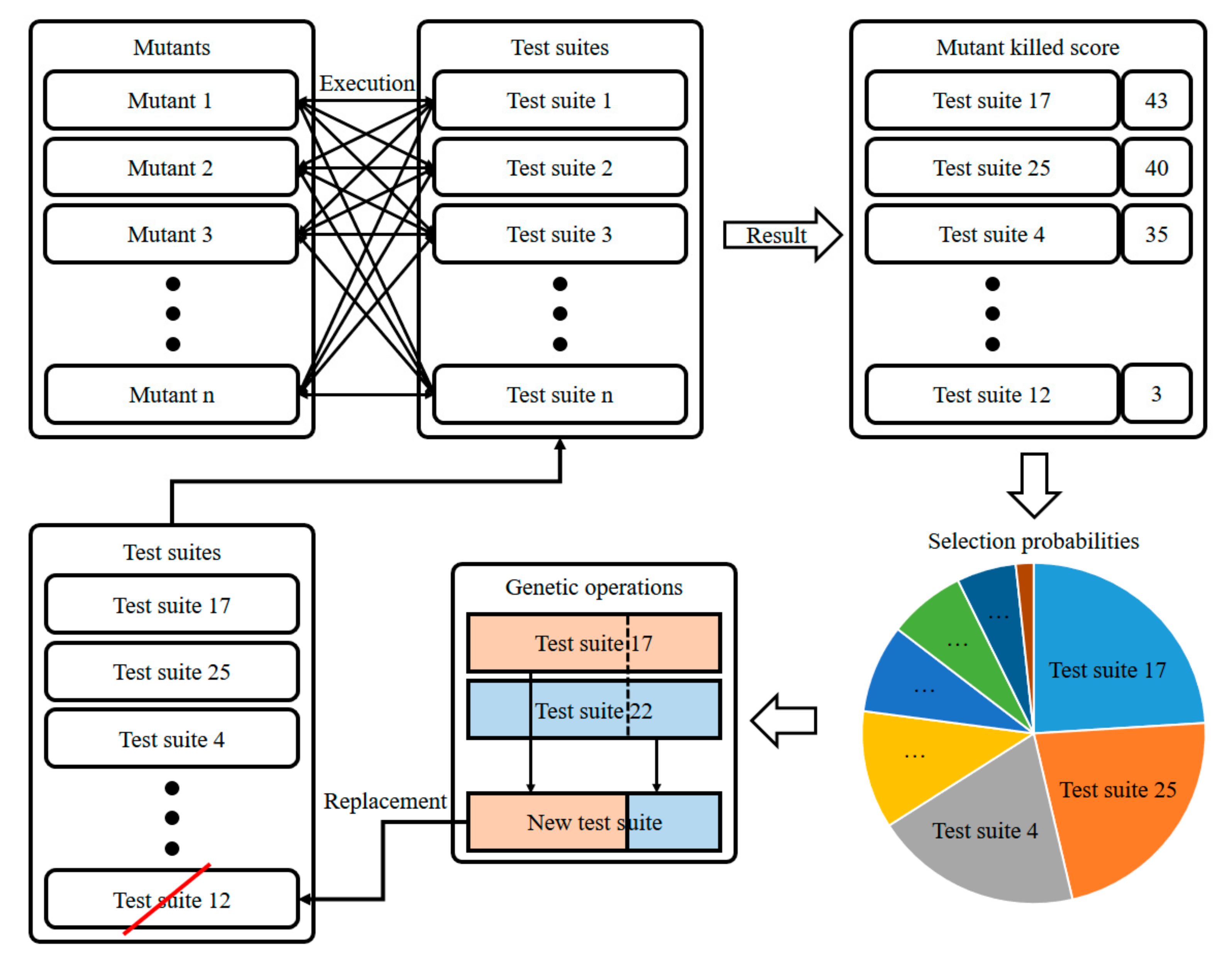Figure 1 is an example of our search-based mutation testing used in this paper. Test suites that kill many mutants have high-quality values, and later receive many opportunities to pass their traits to their offspring when crossovers and mutations (genetic operations) are executed. During this process, low-quality chromosomes (test suites) die out.

Papadakis et al. [23] proposed a fault-localization approach (Metallaxis-FL) based on mutation analysis, which improved the effectiveness of coverage-based fault localization. This method takes advantage of the characteristics of mutation analysis, i.e., that mutants located in the same program statements frequently exhibit similar behavior. Metallaxis-FL executes test cases on mutants and finds mutants whose test results exhibit similar behavior. The position of the mutant is estimated to be the location of the fault. Metallaxis-FL improves the effectiveness of mutation analysis-based fault localization, and also applies mutant sampling to cost reduction. This approach is statistically significantly more effective than the statement-based approach, despite using only 10% of the mutants for fault localization. Almost all of the existing fault-localization approaches require that the test-case execution priority be set to ensure the efficiency of fault localization [17], or that the fault locations be estimated based on test results [23]. One common characteristic of these techniques is that a sufficient number of test cases is required. It can be difficult to apply them to systems in which it takes a long time to run tests.

Liu et al. [24] used a search-based testing technique to improve the test cases and optimize fault localization in the Simulink model. The test-generation algorithm employed featured three fitness functions: coverage dissimilarity, coverage density, and the number of dynamic basic blocks. Coverage dissimilarity focuses on variegation of test execution slices and uses the Jaccard distance [25] to calculate dissimilarity. Coverage density is the mean ratio of all elements covered by the test cases. Campos et al. [26] reported that more accurate statistical rankings were obtained as the coverage density approached 0.5. A dynamic basic block (DBB) [27] is a set of statements that are covered by the same test case. Statistical debugging becomes more effective as the number of DBBs increases. The cited authors established three indicators that increase the variety of tests available for fault localization. However, the technique is applicable to Simulink models rather than to state charts; the guard condition is not considered.

Yoo et al. [17] presented a method using Shannon’s information theory [28] to calculate the expected value passed by each test case and the expected value when a test case fails; this was used to prioritize a test. The work developed tests with high summed suspiciousness expectations for both the next test to be performed and passing or failing. This is a good example of the use of information theory to improve fault-localization prioritization. However, this requires a large number of test suites, such as those of Metallaxis-FL.

In this study, we propose a test-suite generation technique for fault localization at the test-generation stage, which is intended to improve the effectiveness of fault localization. Our method is applied during the test-suite generation phase, and suggests which test suite should be executed next for fault localization. The proposed method aims to estimate fault locations by executing a small number of tests compared to existing fault-localization methods. Our study is a good example of how a test suite for fault localization can be improved using state charts in the presence of a guard condition.

3. Model-Based Test-Suite Generation Using Mutation Analysis

This section describes the model-based test-suite generation based on mutation analysis. The overall concept of the test-suite generation strategy is introduced in Section 3.1. We discuss the algorithms for test-suite generation in Section 3.2 and Section 3.3; Section 3.2 describes the TP generation method, and Section 3.3 describes test suite generation, evaluation, and improvement for fault localization.

3.1. Concept of the Proposed Method

The test-suite generation method proposed in this study began with the question of whether it is possible to use “mutation analysis” to generate test suites that are capable of fault detection and fault localization. The essential aspect of testing techniques that use mutation analysis is that they execute test suites on mutants to predict the results of those test suites [14]. Faults are implemented as artificial defects, and test suites are executed on these faults. Therefore, the test-suite execution results can be predicted, and the test input is adjusted to improve the quality of the test suites. If the search-based technique is combined with mutation analysis, it becomes possible to determine the combinations of test inputs that can kill many mutants using a small number of test suites, and to significantly improve the quality of the test suites [15]. This type of search-based mutation testing is centered around fault detection. However, generating test suites only for fault detection can lead to fault-localization problems. Normally, coverage-based fault-localization techniques, such as mutant coverage or code coverage, find the locations of faults based on the coverage difference between each test suite and a pass/fail determination. If the coverage between passed test suites is similar and the coverage between failed test suites is similar, the technique lacks discrimination power, and it becomes difficult to locate the faults.

Table 1. Example of insufficient fault localization discrimination.

Structural Element	$T_1$	$T_2$	$T_3$	$T_4$	Tarantula Metric
${\mathrm{S}}_1$		●	●		0.5
${\mathrm{S}}_2$	●	●	●	●	0.5
${\mathrm{S}}_3$	●			●	0.5
${\mathrm{S}}_4$(faulty)	●	●	●	●	0.5
${\mathrm{S}}_5$	●		●		0.5
${\mathrm{S}}_6$		●		●	0.5
$Result$	P	P	F	F

shows an example of insufficient discrimination power in fault localization.

Table 1 shows the results of executing ${\mathrm{T}}_1-{\mathrm{T}}_4$ on ${\mathrm{S}}_1-{\mathrm{S}}_6$ and the coverage of each test case. The calculation of the tarantula metric by executing four test cases shows that the tarantula metric is 0.5 for all structural elements. The tarantula metric clearly shows that fault localization did not occur because the passed and failed test cases had similar coverage.

For the above reason, test suites with a diverse range of test coverage are required for fault localization. Typically, many test suites are executed, and the coverage is analyzed to ensure that there is sufficient discriminatory power for fault localization. The method proposed in this study aims to improve the test suites so that fault localization is possible using a small number of test suites. A genetic algorithm, which is a search-based technique, is used to generate test suites that cover a diverse range of mutants and to search the problem space based on test input.

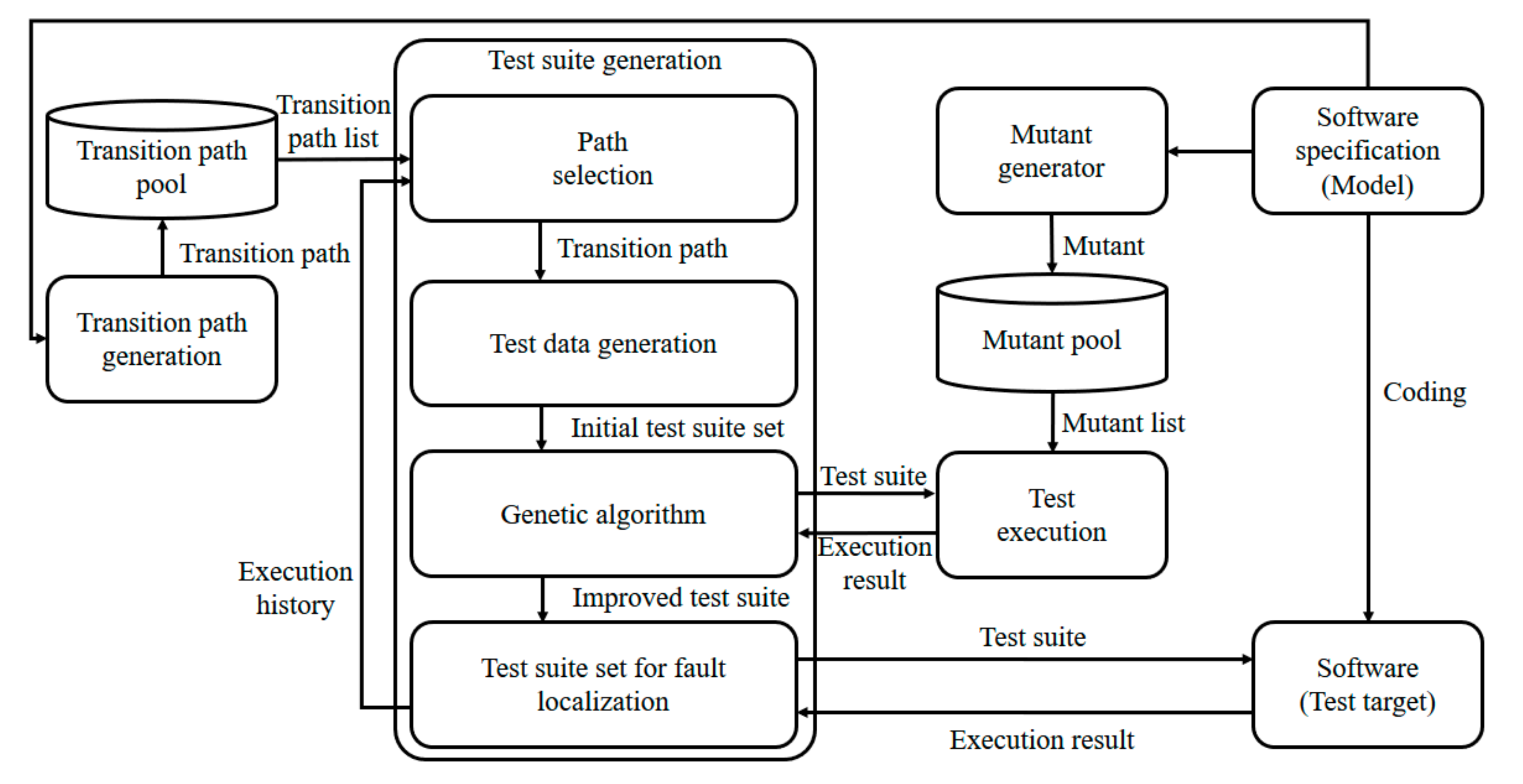
Figure 2 shows the framework of the proposed method, where the TPs are used to generate state chart test suites. During TP generation, paths for generating test suites are generated and saved in the path pool. Paths with a diverse range of coverage are generated so that they will be advantageous for fault localization. The strategy for path generation is described in Section 3.2. The test data generation module generates the initial solution to the genetic algorithm. The initial test suite set is generated based on the path selected in the path pool. The mutant generator generates mutants so that the test input can be developed based on mutant analysis. Each test suite is evaluated via execution with the mutants, and the genetic algorithm is used to pass good traits to later generations via evolution. Test suites with complete evolution are executed on the test target, and the results are saved for use in the next path selection. This process is described in detail in Section 3.3.

3.2. Transition Path Generation

The most important part of test-suite generation for coverage-based fault localization is adjusting the coverage of the test cases and test suites. Here, coverage adjustment is ensured by generating state-chart FTPs. When generating an FTP using a search-based technique, it is possible to generate an FTP that is suitable for the testing goals by assigning scores to fitness functions according to the transition coverage. The basic path generation uses methods from FTP-generation studies [10] to generate paths, and the fitness function is adjusted so that better genes can occur as the coverage density approaches 0.5.

Algorithm 1 is the fitness calculation algorithm. The basic fitness value is 0 when the TP is an FTP and 1 or more when there is an element that cannot be executed. In addition, the fitness value is increased when the TP covers a number which is greater or less than half the total number of transitions. The fitness, which increases due to coverage, is adjusted so that it does not go over 1. Therefore, an FTP has a fitness value between 0 and 1 and is superior to transitions which do not ensure feasibility. This prevents FTPs from being assessed as being inferior to TPs and provides a basis for coverage competition between FTPs.

Algorithm 1. Fitness calculation.

$Where fitness\left(TP\right)=f$ $f=\left\{\begin{array}{ll}f=0,& for FTP\\ f\ge 1,& for non-\mathrm{FTP}\end{array}\right.$ $f=f+\left|\frac{\left(Number of transitions/2\right)-Coverage of TP}{Number of transitions}\right|$

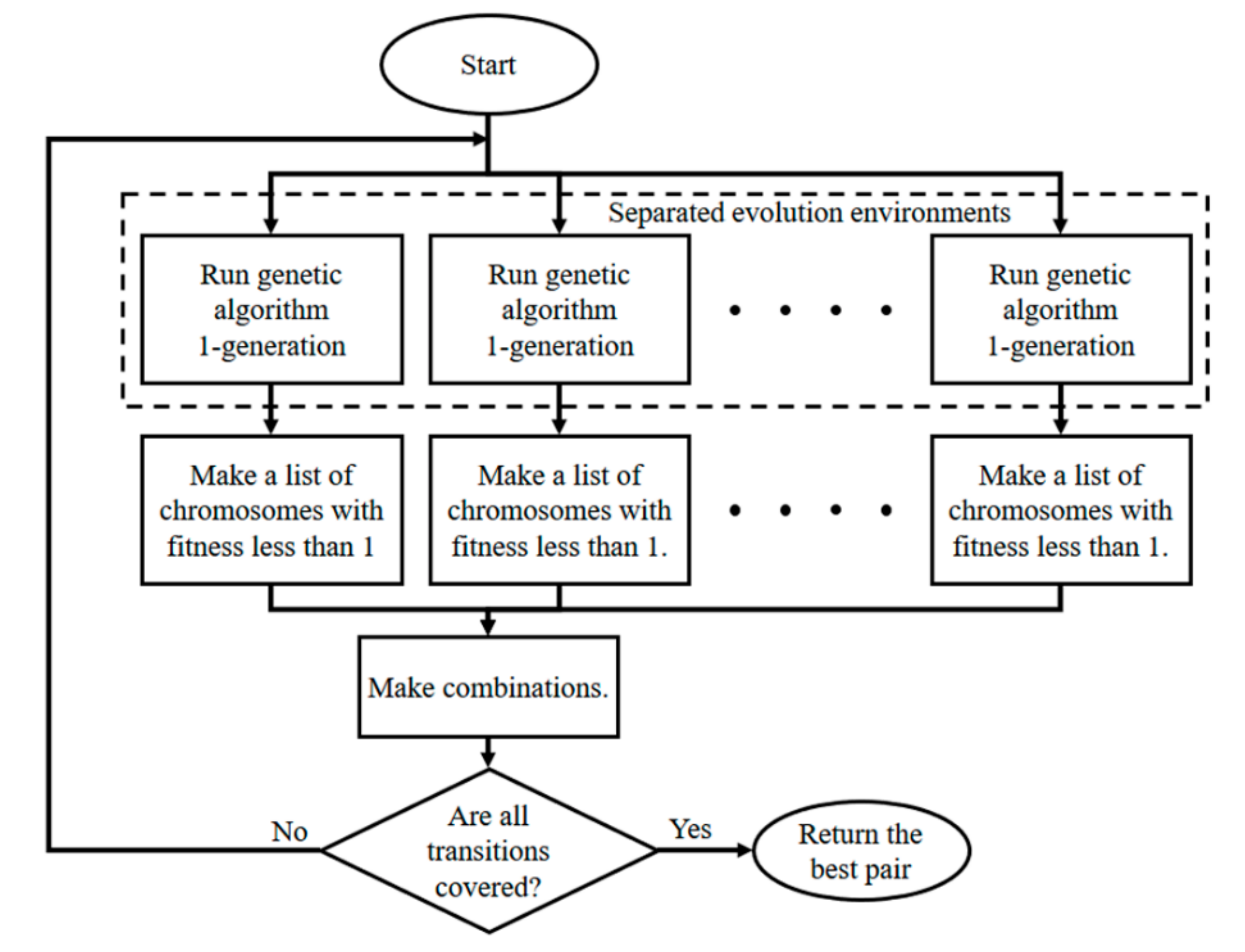
In FTP generation, it is ideal if the density generated is close to 0.5, but if the generated FTPs do not cover all transitions, then test coverage problems can arise. In the most ideal form, a single pair of FTPs covers all transitions. In this study, a pair of separate evolution environments is created to generate an ideal pair of FTPs during test path generation and ultimately to produce the FTP pair with the lowest fitness total out of the FTP combinations, which covers all transitions. Figure 3 shows the algorithm for generating an FTP pair.

Figure 3 shows the organization of the separated genetic algorithm environments. In the same evolution environment, the solution tends to converge to a single point; therefore, it can be difficult to achieve total coverage. The TPs in a separated environment evolve into different forms, and it is easier to achieve coverage of all transitions. When the first round of the evolution process is completed, a list of the TPs that evolve in each environment with a fitness value of less than 1 (i.e., the FTPs) is generated. The evolution process is repeated until a pair that covers all transitions exists between the combinations that can be generated by selecting one from each FTP list. If multiple pairs are found, then the best pair is returned. If a higher-quality FTP is desired, it is possible to use a method that repeats the evolution until the TP pairs that meet the criteria show no improvement for at least a fixed number of generations.

The generated FTPs are saved in the path pool and the process is repeated until the path pool reaches the target number of FTPs. If a large number of FTPs exists in the path pool, it becomes easier to obtain a DBB. However, if the target is set too high, the process takes a long time; thus, it is best to set an appropriate value.

3.3. Test-Suite Generation

The proposed algorithm for FTP-based test-suite generation is classified into two phases. The first phase (Phase 1) focuses on generating test cases that can kill the maximum number of mutants to locate faults. In the second phase (Phase 2), fault-localization test-case generation is performed based on the results of executed test suites generated in the first phase. In each phase, mutation analysis and genetic algorithms are used to improve the quality of the test suite. This section describes the initialization of test suites, genetic operators, and test-suite evaluation algorithms for each phase based on mutation analysis.

3.3.1. Initial Test-Case Generation

The generated test cases and test suites are test inputs based on paths; therefore, they must be generated such that the FTPs can be processed in the appropriate transition order. Each test case must be able to pass transitions that match its order, and each test suite must be able to pass through the TP. To achieve this, we use a boundary value as the initial value. The boundary information is checked based on the transition information, and one of the boundary values is selected at random. However, if test cases are generated solely through a boundary value to ensure that transitions are traversed, a problem occurs whereby some mutants are not handled. For example, when a guard with the condition $x>1$ exists, the value of $x$ as the boundary test-case value for passing through this guard becomes 2. However, when a test case is executed for testing $x\ge 1$, which is a mutant of guard $x>1$, the test case passes without any problem. If a transition for the else branch (in this case, $x\le 1$) does not exist, the mutant cannot be killed. To resolve this problem, failing test cases are inserted between the initial test suites.

Table 2. Improving mutant coverage through failing test cases.

Condition	Mutant	Test Case 1	Coverage	Test Case 2	Coverage
$x>1$	$x\ge 1$	$tc: x=2$		$t{c}_f: x=1$ $tc: x=2$	$killed$
	$x<1$		$killed$		$killed$
	$x\le 1$		$killed$		$killed$
	$x=1$		$killed$		$killed$
	$x!=1$				$killed$
	$x>0$				$killed$
	$x>2$		$killed$		$killed$

shows examples of failing test cases. An input value of 1, which cannot pass the condition, is entered as a failing test case for condition $x>1$ to verify whether the test-case execution fails. Then, the mutant coverage is increased, and the fault-localization accuracy is improved.

3.3.2. Genetic Operations

To generate a test suite that meets the goals of Phase 1 and Phase 2, it is necessary to improve the solution using genetic algorithms. Figure 4 shows the chromosome forms and genetic operators used in this study. In the chromosome-initialization phase, the chromosomes (test suites) are composed of genes that respond to each transition according to the transition order of the given TP, and each gene is composed of a failing test case and a test case. The gene’s test case and failing test case are randomly assigned to one of the boundary values generated.

The chromosome expresses the transition execution order; therefore, the gene’s sequence order changes when a crossover or mutation operation is executed, which is not desirable. When a crossover operation is executed, genes are exchanged between the chromosomes using the same TP and are inserted into the same location, so that the order does not change. When a mutation operation is executed, a randomly selected gene is replaced with a new gene that is suitable for the transition.

3.3.3. Phase 1: Test-Suite Generation for Fault Detection

In the first phase, a high-quality test suite is generated through mutation analysis. The test suites in this phase are aimed toward detecting faults; therefore, they are generated via the genetic algorithm into the form that detects the largest number of mutants. At least one failed test is required to create test suites for fault localization in Phase 2. Phase 1 is a step for finding a failed test. If a failed test was already identified, the process can be skipped.

The overall order of the algorithm consists of initialization, test execution, evaluation, and genetic operation. The test cases generated through initialization and the failing test cases inserted between them are executed with the mutants to determine how many mutants are killed and to evaluate the solution. The genetic algorithm is applied to the best solutions to generate the next generation, which inherits good traits. Test execution is performed on the mutants again to check the quality of the improved solution. Hence, the solution is improved using the genetic operations, and the process is repeated to generate a test input that is advantageous for fault localization. Algorithm 2 shows the pseudo code of the fault-detection test-suite generation algorithm used in this study.

Algorithm 2. Fault-detection test-suite generation.
1:	function FD$\mathrm{TestSuiteGeneration}\left(TP\right)$	>Where $g_{max}$ is the number of max generations
2:	$Chromosome=\mathrm{InitializeTestSuite}\left(TP, p_{num}\right)$	>Where $p_{num}$ is the number of populations
3:	for $g=0$ to $g_{max}$ do	>Where $m_{num}$ is the number of mutants
4:	for p = 0 to $p_{num}$ do
5:	for m = 0 to $m_{num}$ do
6:	if $\mathrm{Execution}\left(Chromosome\left[p\right], mutants\left[m\right]\right)=false$
7:	$Chromosome\left[p\right].quality$++
8:	$Chromosome\left[p\right].mutantcoverage\left[m\right]=true$
9:	end if
10:	end for
11:	end for
12:	$\mathrm{Crossover}\left(Chromosome\right)$
13:	$\mathrm{Mutation}\left(Chromosome\right)$
14:	end for
15:	end function

In Algorithm 2, genetic operations are repeated $g_{max}$ times and the quality of the test suites improves with the number of repeated generations. However, as $g_{max}$ increases, the time required to generate the test suites increases. Therefore, we set the value of $g_{max}$ such that it is suitable for testing. If the test is important, the value of $g_{max}$ can be increased. In each generation, all test suites are performed on all of the mutants. If the results are false (i.e., if the mutant is killed), the quality of the test suites improves. Algorithm 2 is executed twice because it is designed to allow each TP to obtain transition coverage of 50%. Test cases for all transitions are required for fault detection; therefore, random pairs of TPs that cover all transitions are selected, and each is inserted into the algorithm. When this process is complete, the test target program is executed to determine whether the failed test suites exist. If there are no failed test suites, a random TP is selected that is different from the previously selected TP, and the process is repeated until a failed test suite is discovered. If the additional test-suite generation process is repeated, it is more effective to assign high-quality values to chromosomes (test suites) with mutants that were never killed.

Algorithm 3 shows the pseudo code for the test-suite generation algorithm when additional test suites are generated. It differs from Algorithm 2 in that the chromosomes are only assigned scores when a mutant that never previously died is killed. Thus, the test suites are developed so that mutants that were never discovered are found and the fault-detection probability increases. Even if a single failed test suite exists, this process can be repeated if there is a high-risk test target.

Algorithm 3. Fault-detection test-suite generation (additional test suite).
1:	function$\mathrm{FDTestSuiteGeneration}\_\mathrm{Add}\left(TP\right)$	>Where $g_{max}$ is the number of max generations
2:	$Chromosome=\mathrm{InitializeTestSuite}\left(TP, p_{num}\right)$	>Where $p_{num}$ is the number of populations
3:	for $g=0$ to $g_{max}$ do	>Where $m_{num}$ is the number of mutants
4:	for p = 0 to $p_{num}$ do
5:	for m = 0 to $m_{num}$ do
6:	if $\mathrm{Execution}\left(Chromosome\left[p\right], mutants\left[m\right]\right)=false \&\& !mutants\left[m\right].isKilled$
7:	$Chromosome\left[p\right].quality$++
8:	$Chromosome\left[p\right].mutantcoverage\left[m\right]=true$
9:	end if
10:	end for
11:	end for
12:	$\mathrm{Crossover}\left(Chromosome\right)$
13:	$\mathrm{Mutation}\left(Chromosome\right)$
14:	end for
15:	end function

3.3.4. Phase 2: Test-Suite Generation for Fault Localization

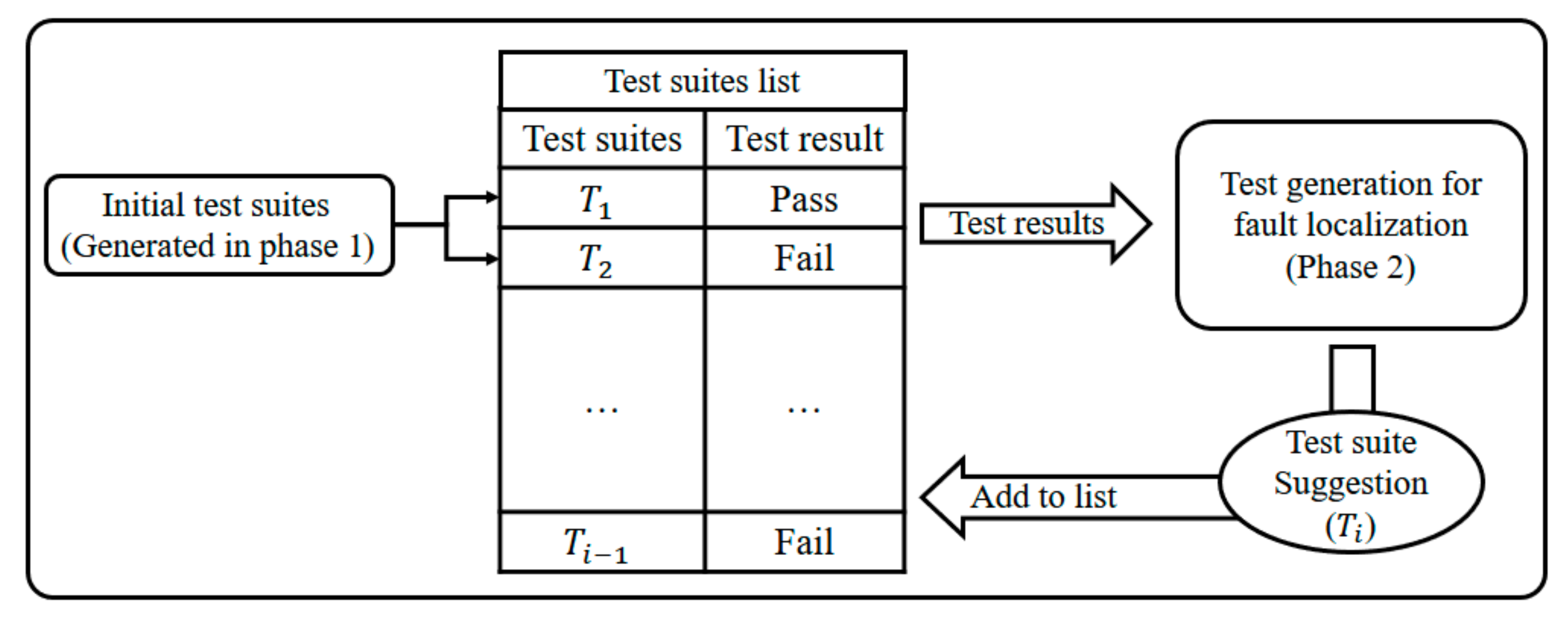
The goal of Phase 2 is to generate test suites that can perform fault localization when one or more test suites fails during Phase 1. Figure 5 shows the test-suite generation process for Phase 2. This phase makes it possible to propose the next test suite for fault localization, based on the results obtained from the Phase 1 test suites, and to perform fault localization with a small number of test suites. Firstly, the next test suite ($T_3$) is created based on the execution results of the test suites created in Phase 1 or previously executed test suites ($T_1$,$T_2$). The test suite ($T_3$) is added to the list, and the next test suite ($T_i$) is created based on all of the executed test suites ($T_1~T_{i-1}$). This process can be repeated as many times as the test designer wishes (e.g., suspiciousness value, number of repeats).

Algorithm 4. Fault-localizing test-suite generation.
1:	function$\mathrm{FLTestSuiteGeneration}\left(TP\right)$	>Where $g_{max}$ is the number of max generations
2:	$Chromosome=\mathrm{InitializeTestSuite}\left(TP, p_{num}\right)$	>Where $p_{num}$ is the number of populations
3:	$\mathrm{SetMutantSuspiciousness}()$	>Where $m_{num}$ is the number of mutants
4:	for $g=0$ to $g_{max}$ do	>Where $t{s}_{num}$ is the number of previous test suites
5:	for p = 0 to $p_{num}$ do
6:	for m = 0 to $m_{num}$ do
7:	if $\mathrm{Execution}\left(Chromosome\left[p\right], mutants\left[m\right]\right)=false$ then
8:	$Chromosome\left[p\right].quality +=mutantSuspiciousness\left[m\right]$
9:	$Chromosome\left[p\right].mutantcoverage\left[m\right]=true$
10:	end if
11:	end for
12:	end for
13:	$\mathrm{Crossover}\left(Chromosome\right)$
14:	$\mathrm{Mutation}\left(Chromosome\right)$
15:	end for
16:	end function
17:	function$\mathrm{SetMutantSuspiciousness}()$
18:	for m = 0 to $m_{num}$ do
19:	for t = 0 to $t{s}_{num}$ do
20:	if $previousTestSuites\left[t{s}_{num}\right].mutantcoverage\left[m\right]=true$ then
21:	if $previousTestSuites\left[t{s}_{num}\right].testResult=false$ then
22:	$mutantSuspiciousness\left[m\right]++$
23:	else
24:	$mutantSuspiciousness\left[m\right]=-1$
25:	break
26:	end if
27:	end if
28:	end for
29:	end for
30:	end function

Algorithm 4 shows the pseudo code of the test-suite generation method for fault localization (Phase 2). The test-suite generation process for fault localization is almost the same as that in Phase 1, in that test suites are executed on mutants and the chromosomes (test suites) are evaluated and developed based on the results. The only difference is the test-suite evaluation method. The mutant suspiciousness used to evaluate chromosomes is the number of times the failed test suites kill each mutant. If failed test suites kill the mutant, the value increases. If passed test suites kill the mutant, the value becomes −1. That is, mutants covered by failed test suites cause test suites to fail, but mutants can be covered by passed test suites (including previously generated test suites), even when they are no longer at all suspicious. Mutants with negative mutant suspiciousness (i.e., mutants no longer under suspicion) can be eliminated to reduce the burden of executing test suites on mutants. This method does not remove mutants that perform as the original software. This may unnecessarily increase the number of executions between mutants and test suites; removal is optimal. If the mutant suspiciousness value is high, there is a high probability that the program under test has the same faults as the mutant. When chromosomes are evaluated, the mutant suspiciousness values are used to assign weights to the mutants. Chromosomes are evaluated as high-quality to the degree to which they cover mutants with high weight values.

To generate fault-localizing test suites, it is important to use an algorithm that evaluates and improves the solution and sets the TPs. In coverage-based fault localization, the tarantula metric uses the coverage of structural elements and whether the test suites pass/fail to calculate suspiciousness. TPs in state charts determine the coverage of the structural elements; therefore, it is important to set TPs for structural element coverage to generate test suites for fault localization.

In this study, two methods were used to set the TPs and the two were compared experimentally. The first method selects TPs based on the transition coverage difference. It uses the Jaccard distance [25] between the TPs used to generate the previous test suites. The Jaccard distance is a method to measure the similarity between two groups, and it has a value between 0 and 1. If the two groups are the same, the value is 1; if the groups contain no common elements, the value is 0. The formula for calculating the Jaccard distance is shown in Equation (2).

$$\mathrm{J}\left(\mathrm{A},\mathrm{B}\right)=\frac{\left|\mathrm{A}\cap \mathrm{B}\right|}{\left|\mathrm{A}\cup \mathrm{B}\right|}.$$

(2)

The Jaccard distance between the TPs used in the previous test suites and new TP candidates is calculated. To set the test paths so that the similarity is not biased in one direction, the method selects the TPs that have the smallest variance in their Jaccard distance with respect to the existing TPs, and the corresponding test suites are generated.

The second method uses entropy lookahead [17]. Entropy lookahead is used to set the priority of the TPs, and the TP with the highest priority is set to generate the test suites. To facilitate a comparison of the two methods, our experimental results are presented in Section 4, and the results of both methods are compared.

4. Experimental Results

4.1. Experimental Set-Up

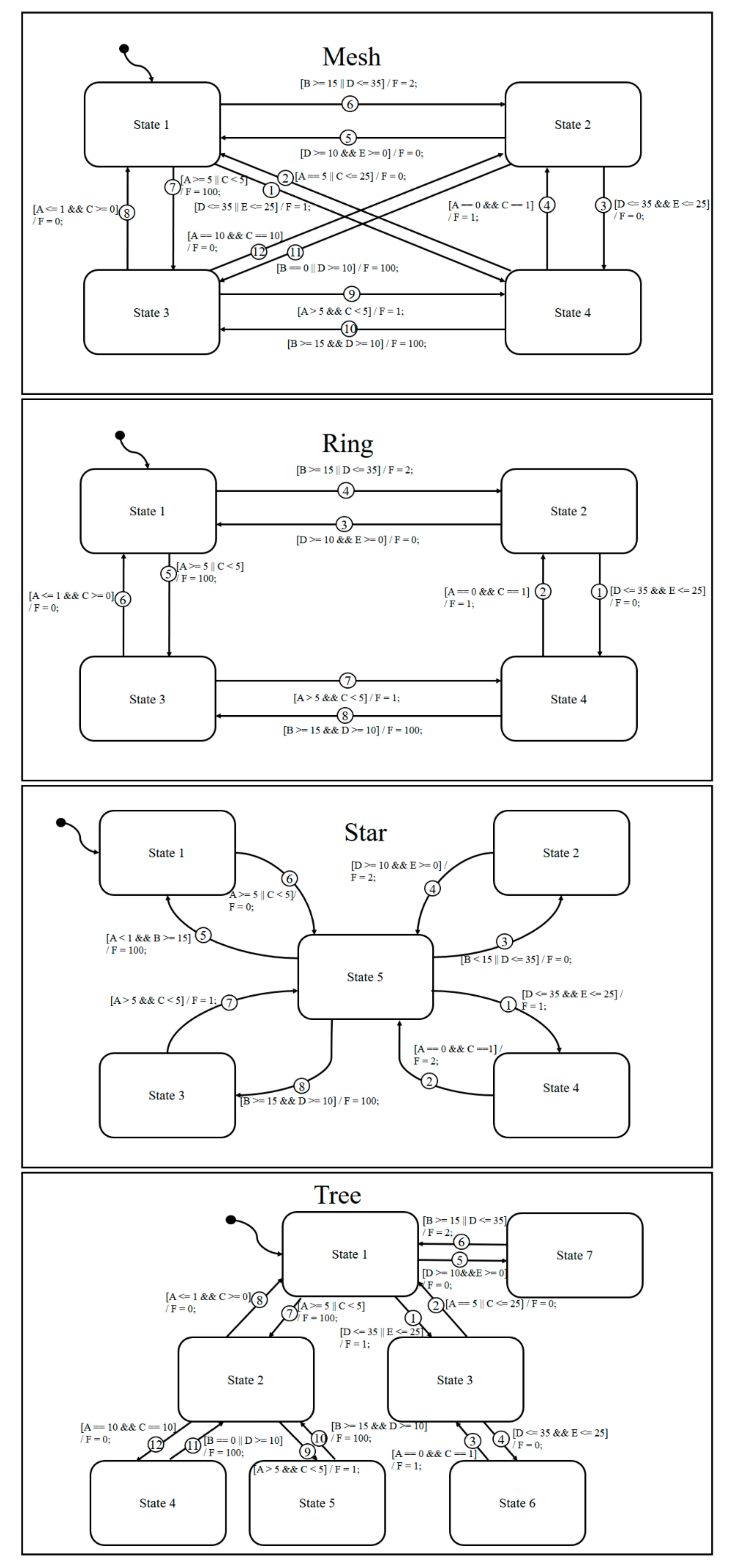
To confirm the effectiveness of the proposed method, tests were performed on four state charts. Figure 6 shows the four state charts used in this study. Star, ring, mesh, and tree state charts were constructed to perform experiments with a variety of forms. The star, ring, mesh, and tree forms were borrowed from different types of network organization and selected to confirm whether fault localization was affected by various organizational forms.

The test-suite generation algorithm was used on the state charts shown in Figure 6. Faulty versions of the state charts (mutants), into which faults were inserted, were used to confirm the effectiveness of the fault detection and fault localization. State-chart information was converted into the extensible markup language metadata interchange (XMI), and a mutant was created by modifying the parsed XMI information. The mutation operator was constructed as in the work of Agrawal et al. [22]. The mutants inserted into the faulty state charts were classified not according to their type but according to the difficulty of killing them. It is difficult to perform experiments on all faulty state-chart cases; therefore, we performed experiments on a limited number of cases. Although the mutation operators may be identical, mutant properties may vary by the guard conditions of different transitions and their priority levels. The sixth transition of the mesh state chart in Figure 6 shows an example of this. In general, transitions with a low number had high priority; therefore, transition 1 had a high priority and transition 6 had a relatively low priority. In state 1, if the guard conditions of transitions 1 and 6 were satisfied simultaneously, it passed through transition 1. Thus, the opportunity to go to transition 6 came only if transition 1′s guard condition D ≤ 35 || E ≤ 25 was false; therefore, transition 6′s condition D ≤ 35 always had to be false. Therefore, if a mutant such as D = 35 occurred at transition 6′s guard, it became an equivalent mutant that could not be killed. For this reason, the experimental targets were selected according to the difficulty of killing mutants, rather than the mutation operators, to make performance comparisons.

In this study, to measure the difficulty of killing a faulty statement (mutant), 2500 random test cases were performed on each faulty version of the program and the number of test cases that killed the fault was calculated. A fault was classified as “hard-to-kill” if it was killed by fewer than 600 test cases, “resistant” if it was killed by 600–1200 test cases, or “weak” if it was killed by more than 1200 test cases.

The experiments were performed on faulty versions of the state charts, to which hard-to-kill, resistant, and weak mutants were introduced as faults. Furthermore, to verify whether the proposed method is valid for non-mutation faults, experiments were also performed for faults that were not generated by mutations. This experimental case can be used to verify that the proposed method is valid, even if the real fault is not a mutation fault.

The experiments were repeated 100 times on each faulty version of the state chart, and 10 fault-localization test suites were generated during each experiment. To generate the test suites, three methods were used: random, Jaccard distance, and lookahead entropy. The random method used random TPs and random boundary test values each time a test suite was generated. The Jaccard distance and lookahead entropy methods (Section 3) were used to set the next TP and improve the test suite through the genetic algorithm. The genetic parameters used are shown in

Table 3. Genetic parameters values used in the experiments.

Genetic Parameter	Value
Crossover probability	1.0
Mutation probability	0.03
Population	20
Max generation	50

.

4.2. Results

Table 4. Summary of experimental results.

State Chart	Difficulty (Killed)	${\mathsf{\tau }}_{\mathbf{R}}\mathit{a}\mathit{v}\mathit{g}$	${\mathsf{\tau }}_{\mathbf{J}}\mathit{a}\mathit{v}\mathit{g}$	${\mathsf{\tau }}_{\mathbf{L}}\mathit{a}\mathit{v}\mathit{g}$	${\mathsf{\tau }}_{\mathbf{R}}\mathit{m}\mathit{a}\mathit{x}$	${\mathsf{\tau }}_{\mathbf{J}}\mathit{m}\mathit{a}\mathit{x}$	${\mathsf{\tau }}_{\mathbf{L}}\mathit{m}\mathit{a}\mathit{x}$	${\mathsf{\tau }}_{\mathbf{R}}\mathit{m}\mathit{i}\mathit{n}$	${\mathsf{\tau }}_{\mathbf{J}}\mathit{m}\mathit{i}\mathit{n}$	${\mathsf{\tau }}_{\mathbf{L}}\mathit{m}\mathit{i}\mathit{n}$
Mesh	W (1750)	0.78	0.98	0.99	0.9	1	1	0.67	0.8	0.875
	R (878)	0.75	0.93	0.91	0.9	1	1	0.6	0.67	0.56
	H (509)	0.68	0.82	0.77	0.78	1	0.875	0.61	0.76	0.64
	N	0.76	0.96	0.9	0.85	1	1	0.67	0.875	0.75
Ring	W (1706)	0.85	1	1	1	1	1	0.7	1	1
	R (818)	0.69	0.89	0.73	0.82	1	1	0.55	0.75	0.56
	H (426)	0.69	0.80	0.65	0.81	1	1	0.64	0.64	0.54
	N	0.72	0.84	0.66	0.85	1	1	0.63	0.69	0.55
Star	W (1719)	0.85	0.98	0.97	1	1	1	0.77	0.9	0.88
	R (856)	0.74	0.91	0.90	0.86	1	1	0.67	0.67	0.625
	H (461)	0.66	0.88	0.80	0.75	1	1	0.6	0.68	0.625
	N	0.73	0.93	0.88	0.79	1	1	0.67	0.65	0.53
Tree	W (1671)	0.87	0.99	0.93	1	1	1	0.69	0.875	0.67
	R (896)	0.73	0.90	0.71	0.89	1	0.92	0.61	0.8	0.6
	H (428)	0.72	0.86	0.71	0.85	1	0.86	0.6	0.69	0.6
	N	0.74	0.88	0.69	0.85	1	1	0.58	0.69	0.53

shows a summary of all of the experimental results. ${\mathsf{\tau }}_R$, ${\mathsf{\tau }}_J$, and ${\mathsf{\tau }}_L$ are the suspiciousness values of faulty statements calculated after performing 10 test suites generated using the random, Jaccard distance, and lookahead entropy methods, respectively. Suspiciousness represents the performance index of each method. A value closer to 1 indicates better performance. The suspiciousness was calculated using the tarantula suspiciousness metric [20]; avg is the average final suspiciousness value of the 100 experimental rounds, and max and min are the maximum and minimum values of the final suspiciousness values. In the table’s difficulty column, W refers to weak, R to resistant, H to hard-to-kill, and N to non-mutant. The numbers inside the parentheses show the number of test cases that killed the mutants out of 2500 random test cases.

In the mesh state chart, the Jaccard distance and lookahead entropy methods both achieved superior results to the random method. In the case of weak and resistant mutants, there were no significant differences between the performances of the Jaccard distance and lookahead entropy methods, but when the faulty statements were hard-to-kill mutants and non-mutants, the Jaccard distance method showed slightly better performance. In the ring state chart, the Jaccard distance method exhibited the best performance overall. In the case of hard-to-kill mutants and non-mutants, the lookahead entropy method achieved worse performance than random test suites. In the star state chart, the Jaccard distance method achieved the best performance. In the tree state chart, the Jaccard distance method exhibited the best performance, and the lookahead entropy method performed the worst.

Table 5. Comparison of performance between methods based on mean suspiciousness value.

State Chart	Difficulty (Killed)	$\frac{{\mathsf{\tau }}_{\mathbf{J}}}{{\mathsf{\tau }}_{\mathbf{R}}}$	$\frac{{\mathsf{\tau }}_{\mathbf{L}}}{{\mathsf{\tau }}_{\mathbf{R}}}$	$\frac{{\mathsf{\tau }}_{\mathbf{J}}}{{\mathsf{\tau }}_{\mathbf{L}}}$
Mesh	W (1750)	25.64	26.92	−1.01
	R (878)	24	21.33	2.19
	H (509)	20.58	13.23	6.49
	N	26.31	18.42	6.67
Ring	W (1706)	17.64	17.64	0
	R (818)	28.98	5.79	21.91
	H (426)	15.94	−5.79	23.07
	N	16.67	−8.33	27.27
Star	W (1719)	15.29	14.11	1.03
	R (856)	22.97	21.62	1.11
	H (461)	33.33	21.21	10
	N	27.39	20.55	5.68
Tree	W (1671)	13.79	6.89	6.45
	R (896)	23.28	−2.73	26.76
	H (428)	19.44	−1.38	21.12
	N	18.91	−6.76	27.53
Average (W)		18.09	16.39	1.61
Average (R)		24.81	11.50	12.99
Average (H)		22.32	6.81	15.17
Average (N)		22.32	5.96	16.79
Average (total)		21.90	10.17	11.64

shows the results of the performance comparison between the methods based on the mean suspiciousness value. The higher the number is, the better the performance of an indicator with a numerator was compared to an indicator with a denominator. The Jaccard distance method was 21% more efficient than the random test suites, and the lookahead entropy method was 10% more efficient than the random test suites. When it became more difficult to kill mutants, the efficiency of the lookahead entropy method decreased.

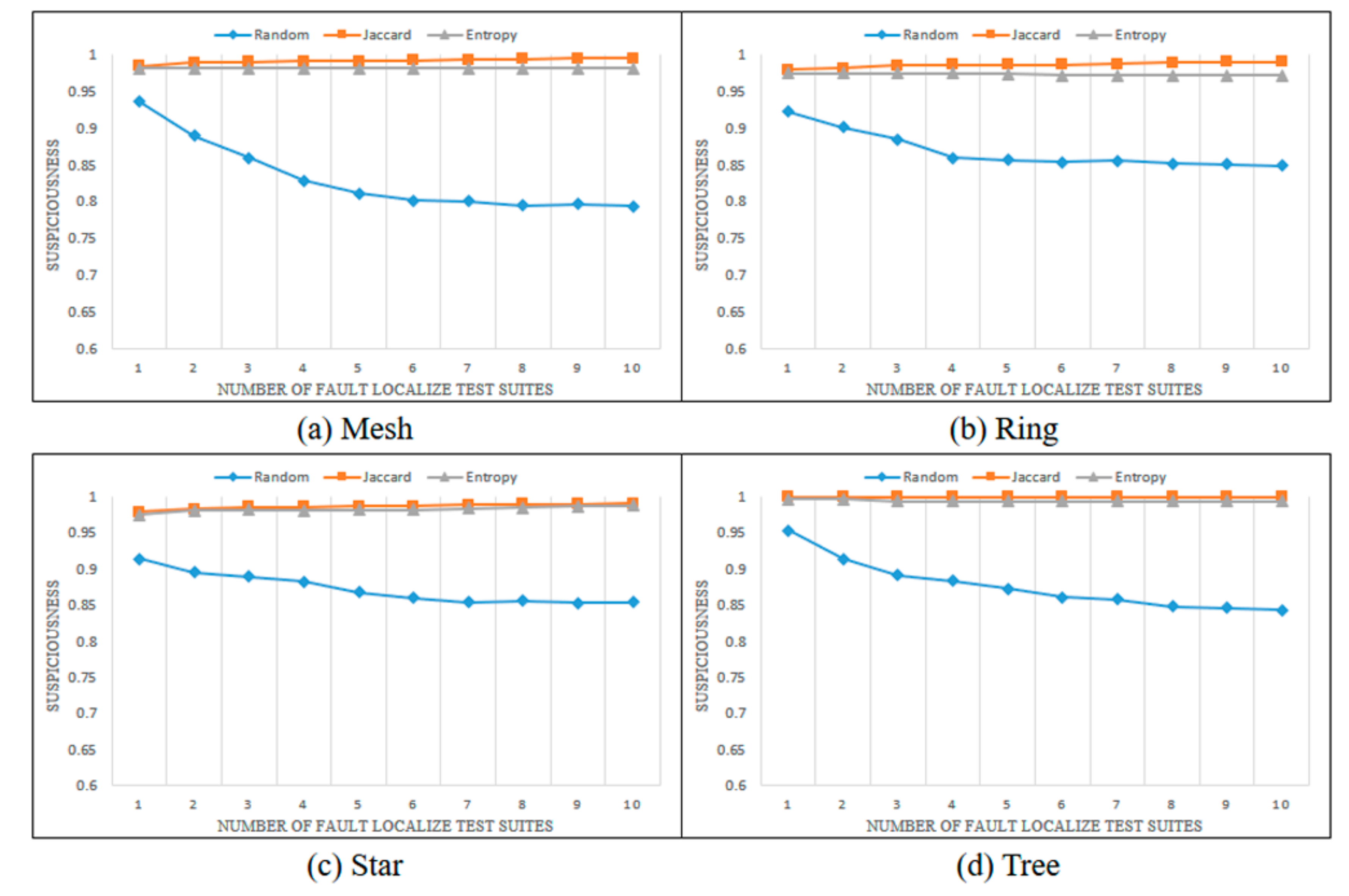
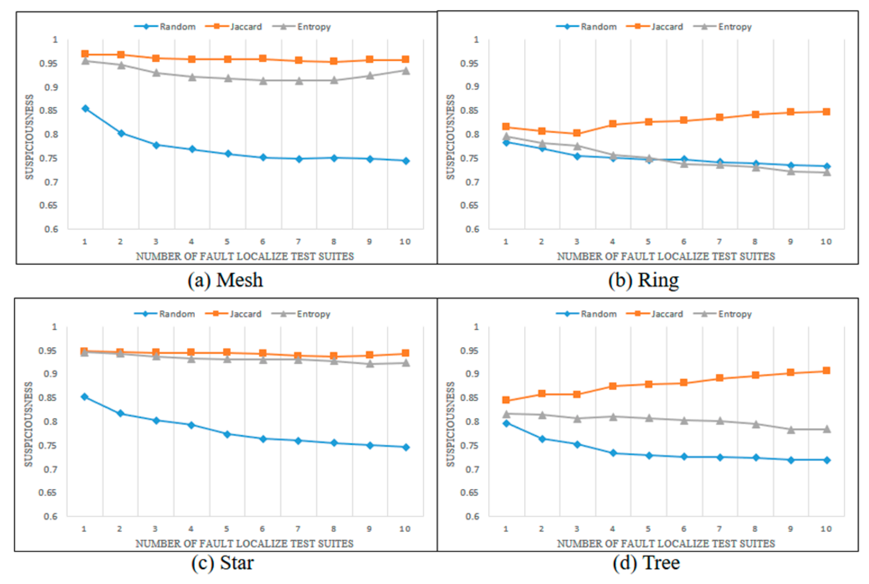
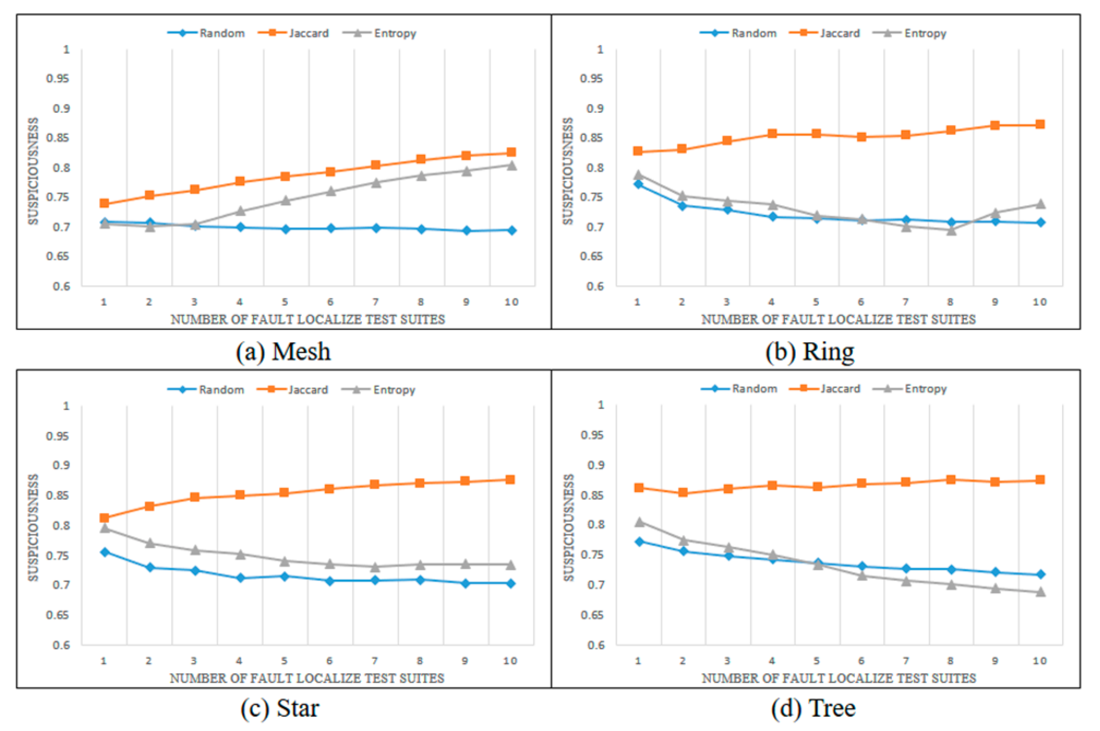
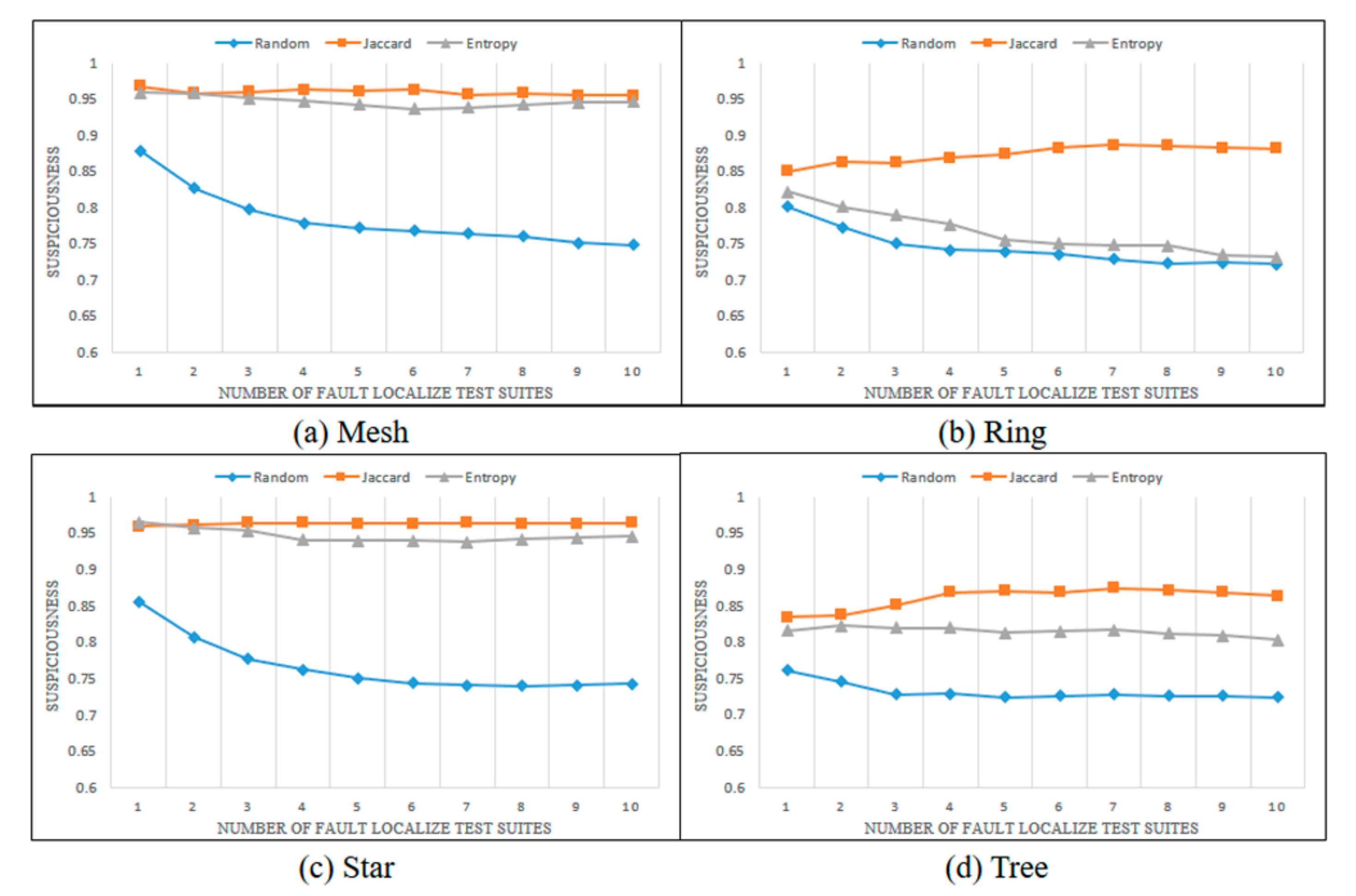
Figure 7, Figure 8, Figure 9 and Figure 10 show the changes in the suspiciousness of faulty statements when executing weak, resistant, hard-to-kill, and non-mutant test suites, respectively. Each time a test case generated by each method is executed, a trend in the suspiciousness of a faulty statement may be noted. This allows evaluation of how efficiently the test cases generated by each method increase the suspiciousness of the faulty statement. Figure 7 shows the results of the weak case in each state chart. In general, there were almost no performance differences between the Jaccard distance and lookahead entropy methods. In the random test suites, the suspiciousness was low during each execution. Figure 8 shows the results of the resistant cases for each state chart. The mesh and star state charts exhibited similar trends to the weak case; however, in the ring and tree state charts, the trend in the lookahead entropy was the same as that of the random method, in which the suspiciousness decreased as the test suites were executed. Figure 9 shows the changes in suspiciousness in each state chart for hard-to-kill cases. When the Jaccard distance was used, the suspiciousness tended to increase. However, when the lookahead entropy method was used, the suspiciousness did not increase in any state charts except for the mesh. Figure 10 shows the changes in the suspiciousness of each state chart for the non-mutant cases. When the Jaccard distance was used, the suspiciousness tended to increase while the rest decreased. Overall, there were no significant differences between the performances of the Jaccard distance and lookahead entropy methods when the faults had low difficulty levels, but the performance of the Jaccard distance method improved as the fault difficulty increased.

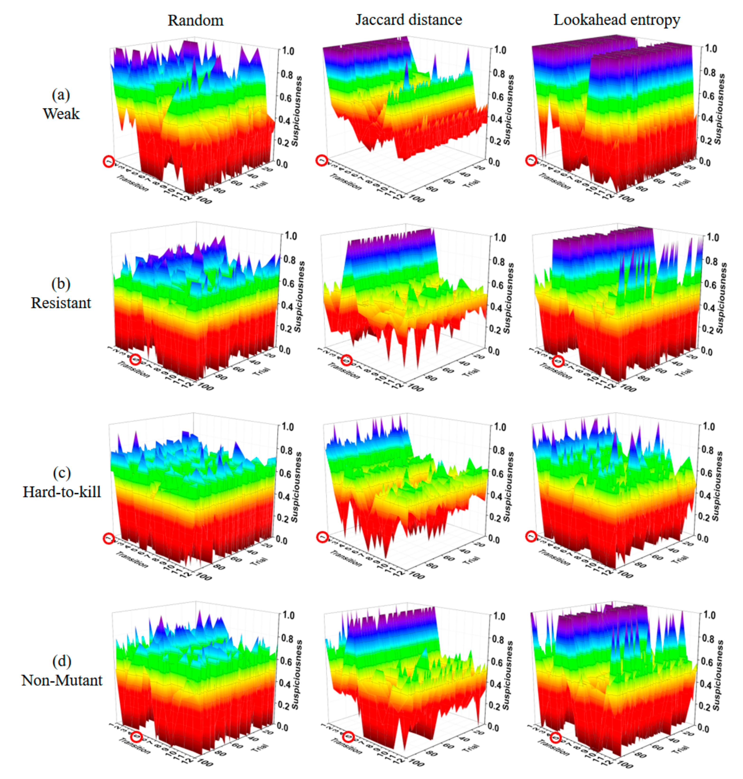
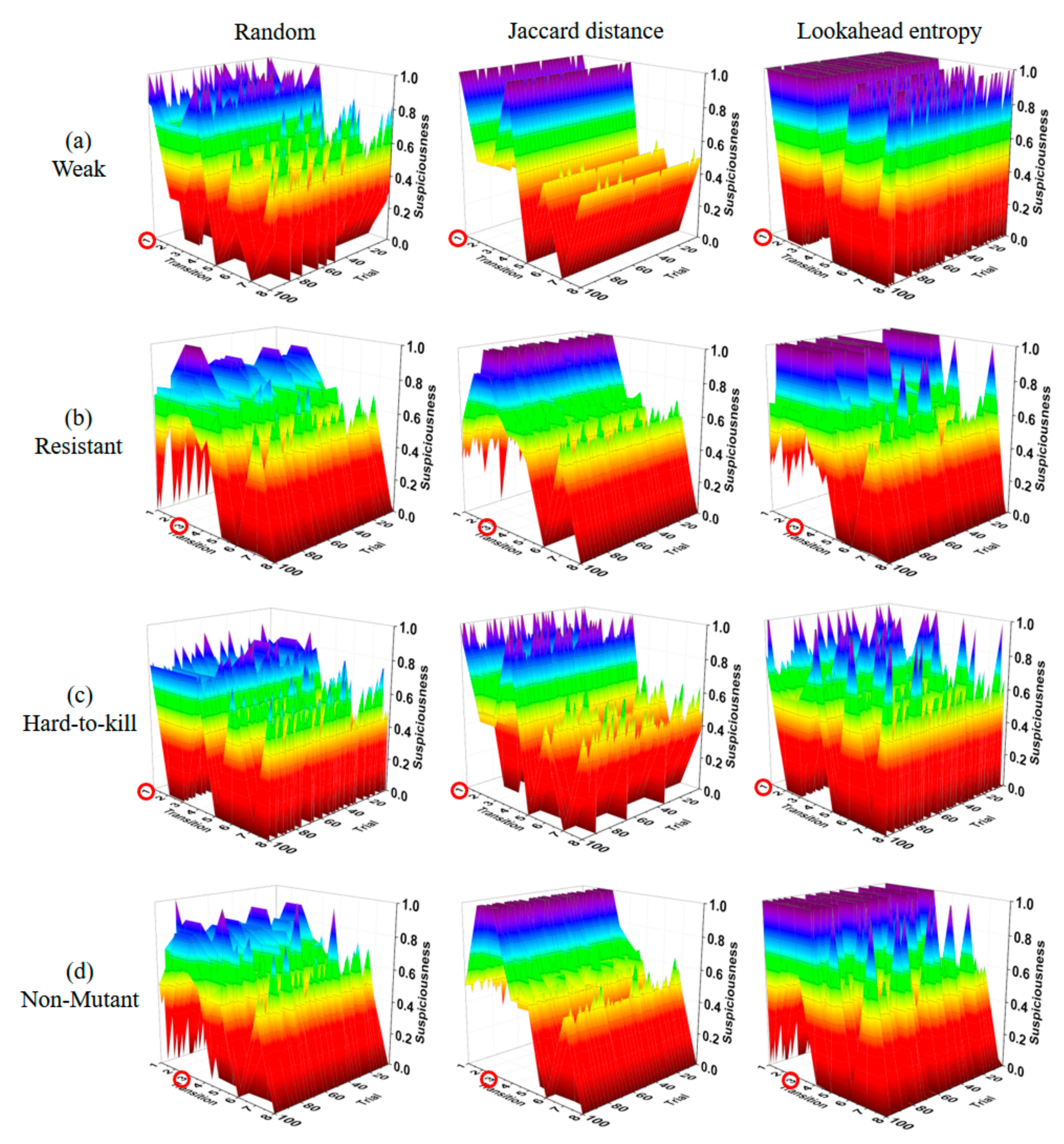
Figure 11, Figure 12, Figure 13 and Figure 14 show the suspiciousness of the transitions after completing the execution of the 10 test suites generated using each method in 16 cases. The graph shows the difference between the faulty statement and the other statements. The clearer the difference between the suspiciousness of a faulty statement and the suspiciousness of other statements is, the better the performance was. The transition numbers of transitions that contain faults are circled. In the results from the random test suites, the suspiciousness was sometimes higher in non-faulty transitions than in faulty transitions. Ten test suites were considered insufficient to perform fault localization through random test suites alone. When the Jaccard distance method was used, the suspiciousness values of non-faulty transitions were distributed evenly. However, when the lookahead entropy method was used, the suspiciousness values of the non-faulty transitions were not even. The most extreme case of this phenomenon is shown in Figure 12a, where weak faults were inserted into the ring state chart. The suspiciousness of the faulty transition tr1 was satisfactory; however, in other transitions, there were several non-faulty transitions with suspiciousness values of 1. Furthermore, most other cases exhibited similar suspiciousness values for faulty and non-faulty transitions, or non-faulty transitions had higher suspiciousness levels. The mean values of results obtained using the Jaccard distance and the lookahead entropy did not differ significantly. However, the Jaccard distance results were stable, whereas the lookahead entropy data were not because entropy was prioritized based on the sum of suspiciousness when the result of the next test was pass or fail. Figure 13 and Figure 14 also show the elements that pose obstacles to fault localization for different types of state charts. In the star state chart, tr1 must be executed first to execute tr2; therefore, if there is one faulty transition between tr1 and tr2, there is no suspiciousness discrimination ability for tr1 and tr2. Similarly, in the tree state chart, for two pairs of transitions (tr9, tr10 and tr11, tr12), individual transitions tend to have the same suspiciousness as the other member of the pair. Even if these elements were excluded, we obtained insufficient fault-localization discrimination. Therefore, Jaccard-distance-based TP selection enabled superior fault localization.

5. Conclusions

This paper proposed a two-phase method for generating test suites for fault localization in state charts. The method was designed so that, in the first phase, at least one test suite that passes and one test suite that fails are generated to calculate suspiciousness for fault localization. In the second phase, the test suites are generated based on the results of executing test suites generated during the first phase. The Jaccard distance and lookahead entropy methods are used to select paths to generate the next test suites in this phase. Furthermore, a genetic algorithm is executed based on mutation analysis to generate test suites for fault localization.

To confirm the effectiveness of the proposed method, four levels of faults were inserted into four types of state charts; thus, 16 faulty versions of state charts were used in the experiments. The experimental results confirmed that the method that used the Jaccard distance was more effective than the method that used lookahead entropy, and the suspiciousness of faulty statements increased by more than 21% compared to random test suites based on boundary values. Furthermore, when paths selected via Jaccard distance were used to generate test suites, the suspiciousness of non-faulty statements was distributed more evenly than when using the random or lookahead entropy methods. We also confirmed that our method had the ability to discriminate between faulty statements and non-faulty statements.

Future studies should focus on further reducing the number of test suites for fault localization. Different types of path generation or selection methods could reduce the number of test suites required for fault localization. More effective search-based algorithms should be considered to achieve this goal.