1. Introduction
Supplier selection under various conditions and selection criteria has been an important issue in supply chains since procurement costs are the dominating cost factor in many sectors. Many criteria can be considered in supplier selection such as quality, price, delivery performance, and distance to the buyer. In this study, we consider a case in which the buyer needs to optimally choose a set of suppliers and order quantities from these selected suppliers to fulfill the demand for multiple items in multiple time periods. This case is common when suppliers sell standard components with identical features and compete solely on pricing policies and closeness to potential buyers. In this problem, buyers have to make three basic decisions: (1) selection of suppliers to satisfy demand; (2) order lot sizes from each supplier; (3) routes to collect orders by multiple vehicles. In making these decisions, buyers will consider price discounts, transportation, and inventory holding costs.
We develop a mixed-integer programming model to select the best set of suppliers and to determine the proper allocation of order quantities while minimizing the total cost which consists of the ordering, inventory holding, transportation (routing), and purchasing costs under suppliers’ capacity and price discount constraints. The purpose of this study is to construct a supplier selection and lot-sizing model with price discounts in a multi-supplier, multi-component, multi-period, and multi-vehicle environment in order to minimize total cost over a planning horizon. The model permits price discounts offered by different suppliers for different components. Multiple sourcing and multiple components are considered in the model to represent a more general situation.
The paper is organized as follows. In
Section 2, literature on supplier selection, order allocation problems, and traveling purchaser problems are briefly reviewed. In
Section 3, problem formulation and a mathematical model are described in detail.
Section 4 is devoted to a numerical example and its solution. In
Section 5, scenario analysis is provided to analyze the effects of the basic cost factors of the model on the optimal solution. Finally, the findings and conclusions of this study are presented in
Section 6.
2. Literature Review
Determination of the order quantity among suppliers takes an important place in the relations of suppliers and buyers. As the purchasing decisions are based on multiple suppliers, companies split their orders among suppliers. Therefore, the power of suppliers over the buyers reduces. This is how companies can reach low prices. Buyers split order quantities among selected suppliers to keep secure working with them [
1].
Several studies on the supplier selection and order allocation problem have been conducted by several researchers [
1,
2,
3,
4,
5,
6,
7,
8,
9,
10]. Mansini et al. [
11] studied a procurement problem simultaneously taking into consideration the transportation and purchasing costs, introducing both an integer programming model and a heuristic solution. Inventory holding cost has also been taken into consideration in some studies. Mendoza and Ventura [
12] develop two mixed-integer nonlinear programming models for supplier selection and order allocation while minimizing total cost, which consists of ordering, inventory holding, and purchasing costs subject to quality and suppliers’ capacity constraints. Cárdenas-Barrón et al. [
13] consider the multi-product multi-period inventory lot-sizing with supplier selection problem. Their model considers ordering, holding, and purchase costs.
Some articles tackle purchasing, transportation, and inventory decisions simultaneously. Mendoza and Ventura [
14] propose a mixed-integer nonlinear programming model in order to allocate order quantities to the selected set of suppliers considering purchasing, transportation, and inventory costs subject to quality and suppliers’ capacity constraints. Hammami et al. [
15] present a mixed-integer programming model for the supplier selection problem with multiple products and multiple periods in an international context, which takes into account inventory and transportation decisions. Pazhani et al. [
16] introduce a mixed-integer nonlinear programming model which includes transportation costs. Lee et al. [
17] presented a mixed-integer programming model to solve the lot-sizing problem with multiple suppliers, multiple periods, and quantity discounts. Their objective was to minimize the total cost, which includes ordering, inventory holding, purchasing, and transportation costs. However, price discount was not included in their model. Our study considers ordering, purchasing, transportation, and inventory holding costs, as well as price discounts.
Many papers have addressed the traveling purchaser problem. Their models were handled with different constraints [
18,
19,
20,
21,
22].
In the literature, there are studies which separately examine either the supplier selection, order quantity allocation or traveling purchaser problems mentioned above; however, no studies have been found that integrate these problems. This study aims to fill this gap using a single integrated mathematical programming model. Furthermore, in the literature, decision models and techniques for supplier selection do not often consider issues related to inventory, vehicle routing, and price discounts simultaneously. This study deals with all these real-life constraints and situations.
In this article, a mixed-integer nonlinear programming model is proposed to select the best set of suppliers and determine the proper allocation of order quantities while minimizing total cost, including the annual ordering, inventory holding, purchasing, and routing costs under suppliers’ capacity and price discount constraints.
3. Problem Formulation
The problem consists of a set of vehicles belonging to a buyer, a group of suppliers, and a group of components. It is assumed that the planning horizon consists of more than one period. This study considers a multi-supplier, multi-vehicle, and multi-component environment. Suppliers offer different discount intervals to the buyer based on the total amount of products that the buyer purchases in each period.
This study proposes a model that helps the buyer to distribute the demand among multiple geographically scattered suppliers, and they propose different price discount intervals for the components. In response to the buyer’s demand for each component, the selection of suppliers and order sizes are integrated with the determination of optimal routes of multiple vehicles that will collect orders periodically.
The components ordered from any supplier are priced separately over the non-discounted prices and the total price for all products is calculated first. Then, if the total amount falls within a certain discount range within the scope of the discount policy applied by the supplier, the discount is applied at the percentage determined for that discount range. How much of the component will be taken from the supplier is determined by the capacity of the supplier and the total cost of the product. If the same products are available from more than one supplier, the quantities of these products in these suppliers may be different. The model differs in that it allows each component to be purchased in different quantities from different suppliers. That is, in the model, the buyer is not limited to the ability to buy a component from only one supplier, but is allowed to purchase different amounts of a component from different suppliers in the most cost-effective way. In this model, demand is deterministic. A component can be supplied from more than one supplier, and more than one component type can be supplied from a supplier. Therefore, there is no requirement to obtain a product from only one supplier. In addition, different amounts of a component may be obtained from other suppliers where the product is not available from that supplier. Therefore, the demand is met by the supplier with sufficient capacity. At any given time, any supplier can only be visited by one vehicle, and the vehicle collects all components ordered from the supplier. If the current capacity of a vehicle is not sufficient to collect all of the products ordered from any supplier, then the vehicle does not make a partial collection and that supplier is visited by another car with sufficient capacity. The assumptions used in the problem are shown in
Table 1.
Mathematical Model
A mathematical model is developed to determine an optimal set of suppliers, order quantities, and vehicle order collection routes. The total cost is defined as the sum of purchasing, ordering, inventory, and transportation costs. Transportation (routing) cost is determined by multiplying the transportation cost per unit distance and the distance matrix values. There is also a fixed cost added to the transportation cost when a vehicle starts a route. The purchasing cost consists of the discounted total amount of the products ordered from a supplier in a period. Ordering cost can be defined as the cost of placing a product from a supplier. Inventory costs may be preferable in order to benefit from the price discount offered by suppliers.
Let be the set of components to be purchased, let be the set of suppliers to choose from, and a depot (buyer) indexed by 0, let be the set of supply periods, let be the fleet of identical vehicles available for the service, and let be the set of discount intervals offered from suppliers. Each component can be purchased from a group of suppliers depending on whether they have the component. Each component can be supplied from more than one supplier, and the order size of a component is determined based on the capacity of the supplier and total cost of the component. The unit of the component can be found at supplier . The distances of suppliers to the buyer are shown in the distance matrix Dmn. There is a fixed cost per period for each vehicle as independent of distance traveled. The notation used to express equations of the mathematical model is as follows:
Notation:
Indices:
i: suppliers (i = 1, 2, …, I)
j: components (j = 1, 2, …, J)
k: discount intervals (k = 1, 2, …, K)
t: planning periods (t = 1, 2, …, T)
f: vehicles (f = 1, 2, …, F)
m: starting supplier (m = 1, 2, …, I + 1)
n: ending supplier (n = 1, 2, …, I + 1)
Parameters:
M: a large number
: demand for component j in period t (units)
: capacity of supplier i for component j in period t (units)
: undiscounted unit price of component j from supplier i (unit of currency/unit)
: discount ratio of supplier i for kth discount interval (%)
: lower limit of kth discount interval of supplier i (unit of currency)
: unit holding cost of component j (unit of currency/unit/period)
: fixed ordering cost for supplier i (unit of currency/order)
: distance matrix between the depot and suppliers (distance unit)
c: unit transportation cost per unit distance (unit of currency/distance unit)
w: fixed cost of a vehicle per time period (unit of currency/period)
: maximum loading capacity in weight for vehicle f (weight unit)
: unit weight of component j (weight unit/unit)
Objective Function:
subject to
In the integer programming model above, Equation (1) states the objective function which is the sum of purchasing, ordering, inventory holding, fixed vehicle, and transportation costs. Equation (2) is the set of inventory balance equations for all components and time periods. Although Equation (3) states that there is zero inventory at the beginning of the first period, this restriction can easily be removed if necessary. Similarly, Equation (4) closes the last period with no inventory in hand. Equation (5) ensures that order quantities do not exceed the corresponding supplier’s capacity. Equation (6) determines whether there is an order from a supplier in any given period. Equations (7) and (8) calculate the total amount ordered from each supplier before discount and after discount, respectively. Discount intervals applied to each component are determined in Equations (9) and (10). Equation (11) is a set of subtour constraints ensuring that a vehicle visits at most only one supplier in one step at any period. Equation (12) ensures that if a vehicle is used to collect orders, then the starting point of the route of that vehicle must be the warehouse. Equation (13) states the flow balance equations meaning that if any vehicle goes to any supplier in any period of time, it must surely go from one supplier to another and finally return to the warehouse. Equation (14) prevents bi-directional visits between any pair of suppliers as required in the traveling salesman problem. Equation (15) ensures that only suppliers with orders are visited by a vehicle. The maximum loading capacity constraint of a vehicle is expressed in Equation (16). Equation (17) calculates the value of binary variable Yft based on each vehicle’s route.
4. A Numerical Example
A numerical example is introduced to illustrate how the developed model works. The numerical example includes 4 suppliers, 2 vehicles, 4 components, and 3 discount intervals for each supplier and 3 time periods. Unit transportation cost per unit distance is 10; fixed cost of a vehicle is 20; maximum loading capacity for vehicle f is 250; unit weight of component
j is 3; unit holding costs of component
j are h
1 = 10, h
2 = 20, h
3 = 5, h
4 = 10; and ordering costs for suppliers are o
1 = 10, o
2 = 20, o
3 = 15, o
4 = 25.
Table 2,
Table 3,
Table 4,
Table 5,
Table 6 and
Table 7 show the values used in the numerical example for demand sizes of components, suppliers capacities, undiscounted unit prices, distance matrix, price discount ratios, and price discount interval lower limits respectively.
By using the numerical example data, the mathematical model is solved in the LINGO 9.0 program. The optimal solution of the model is given in the following tables.
In
Table 8, it is seen how much of the components are taken from suppliers in each period.
Table 9 shows the undiscounted total amounts of the components ordered from each supplier.
Table 10 shows the discounted total amounts of the components ordered from each supplier. The discounted total amounts are calculated based on undiscounted total amounts.
The routes followed by the vehicles are shown in
Table 11. For example, according to
Table 11, the second vehicle goes from warehouse to Supplier 2, 3, and 4 in succession at period 1. At the end of this route, this vehicle turns back to the warehouse.
5. Scenario Analysis
To demonstrate the behavior of the model proposed, scenarios are presented in this section. By changing the values of the parameters in the sample application, the effect of this change on the optimum solution is investigated. In Scenario 1 and 2, the model is tested by changing the values of some parameters. Scenario 3 and Scenario 4 demonstrate the effects of inventory holding cost and transportation cost on the total cost.
Scenario 1: Supplier 1 offers the lowest unit price for all components.
Table 12 shows the undiscounted unit prices for this scenario.
In
Table 13, it is observed that the order quantities allocated to Supplier 1 are increased. According to
Table 14, the revised route has a visit to Supplier 1 due to a decrease in purchasing cost. The decrease in purchasing cost also lowers the total cost. The calculated amounts and the change of vehicle routes are shown in the following tables. The optimum solution is obtained as follows.
Scenario 2: By replacing the Dmn matrix as follows, Supplier 2 is moved further away than the other suppliers.
As a result of changing the
Dmn matrix as shown in
Table 15, Supplier 2 is taken away from other suppliers.
On the basis of these data, Supplier 2 is not being ordered from and the components previously ordered from Supplier 2 have begun to be ordered from other suppliers.
Table 16 and
Table 17 summarize the optimum solution for this scenario.
As predicted, the resulting impact of this change is the removal of Supplier 2 from the list of selected suppliers. According to
Table 17, vehicles do not visit Supplier 2.
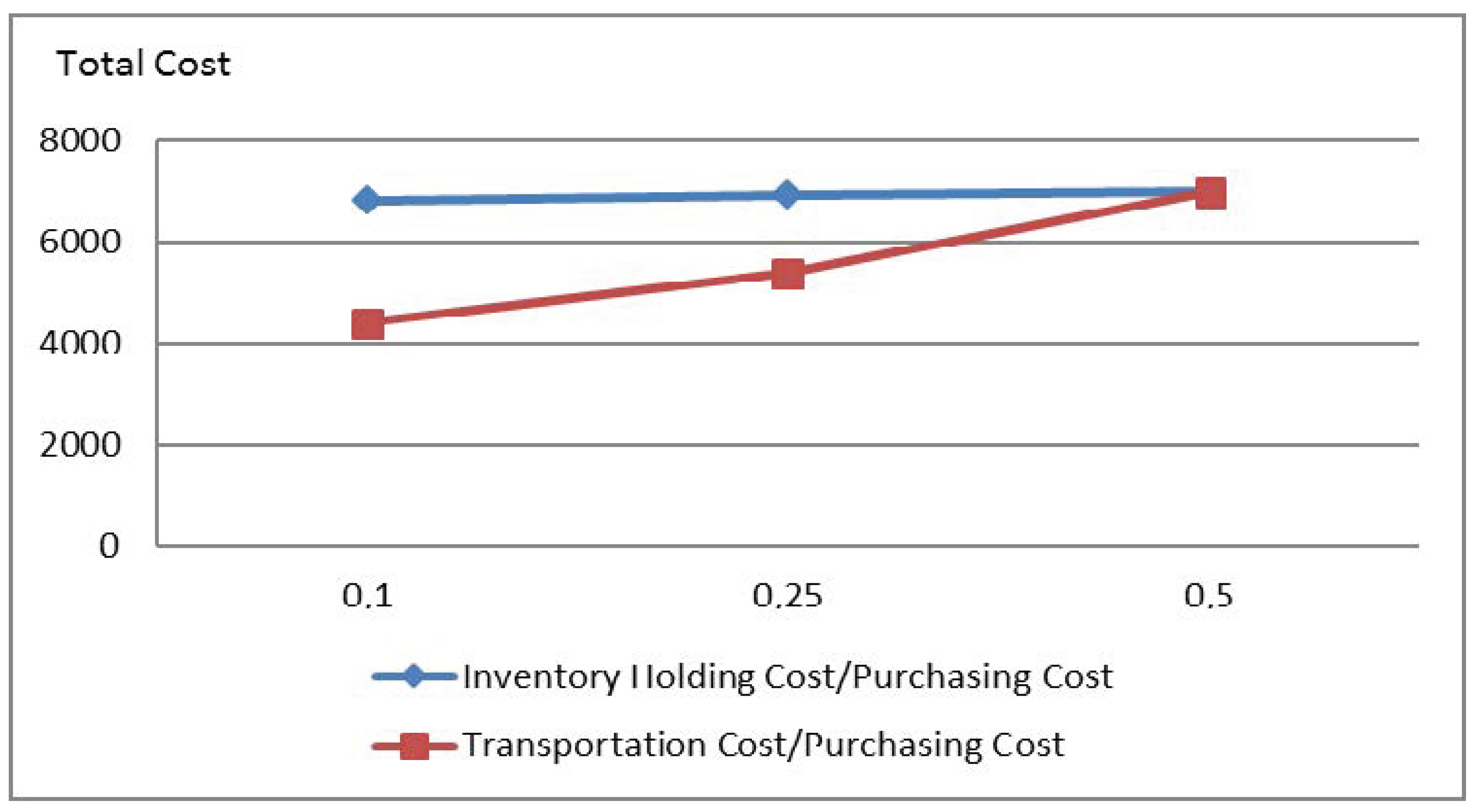
Scenario 3: Changing the ratios of inventory holding cost over purchasing cost.
The data are kept the same as the numerical example.
Pij values are given in
Table 18. The effect of the proportional change on total cost is observed by changing the ratio of unit transportation cost per unit distance to the undiscounted price per unit of component at 50%, 25%, and 10% rates.
Scenario 4: Changing the ratios of transportation cost over purchasing cost.
The data are the same as the previous scenario. The effect of the proportional change on total cost is observed by changing the ratio of unit transportation cost per unit distance to the undiscounted price per unit of component at 50%, 25%, and 10% rates.
Figure 1 illustrates the effects of changing the ratios of transportation cost and inventory holding cost over purchasing cost.
Based on the results of Scenarios 3 and 4, we observe that transportation costs have a larger impact on the total cost as compared to inventory holding costs. This result suggests that buyers should work with suppliers with closer distance and create a supplier network with short distances between suppliers.
6. Conclusions
In this paper, a mixed-integer nonlinear programming model is proposed to select the best set of suppliers and determine the proper allocation of order quantities while minimizing the total cost of ordering, inventory holding, transportation (routing) and purchasing costs under suppliers’ capacity constraints and price discounts. The developed mixed-integer programming model is solved by LINGO optimization software.
Our research makes contributions to the existing literature in various ways. First, supplier selection and order allocation problem with price discount and traveling purchaser problem were integrated into a dynamic framework. In addition, price discounts, stock, and routing decisions are also included in the problem. Second, a new mixed-integer linear programming model was developed to find the order quantity allocated to each supplier in each period. The model also determines the most suitable suppliers to work with. Third, our proposed integrated approach to supplier selection can significantly reduce the total procurement costs as it considers all related costs to procurement. Fourth, our scenario analysis shows that transportation costs may play a significant role in determining the optimal set of suppliers.


