1. Introduction
Knee osteoarthritis (OA) is the most frequent form of arthritis among older people. It is the main cause of physical disability and activity limitation among older people. In 2000, 13% of the population in the U.S. were aged 65 and above, and more than half of this population had osteoarthritis in at least one of their joints [
1]. It is estimated that the number will increase to at least 20% of the U.S. population, which is ~70 million people, and will have crossed 65-year-olds by 2030, and will be at risk of suffering from OA [
1]. Statistical analysis indicated that the U.S. incurred an approximate cost of
$336 billion, equivalent to 3% of its gross domestic product (GDP), to treat patients suffering from arthritis in 2004 [
2]. The OA disease has been a major cause of increased economic expense burden on the society in the form of early retirement, increased absenteeism from work, as well as the high cost associated with joint replacement [
3].
The cause of OA is still unknown, and there is no effective treatment found yet that may slow the progression of OA disease [
4]. Measurement of cartilage damage is used as an essential endpoint to assess the structural change of OA progression in clinical studies. The decrease in cartilage is associated with the progression of the OA pathology [
5]. According to the previous study [
6], changes in the whole knee cartilage layer may demonstrate certain patterns along with the development of the OA. For example, the cartilage regions that bear more weight tend to have more cartilage loss. Very limited research has been done on using machine learning method to model the cartilage changing patterns. In clinical research, magnetic resonance (MR) is considered as a technology that has noninvasive nature which can be used to quantify cartilage. However, it is time-consuming to measure the morphology of cartilages using MR images. The manual segmentation of a 3D knee MR series may take up to 6 h. Moreover, operators need extensive training [
7] to accurately measure cartilage.
For the past decade, scientists have conducted research to find efficient and reliable methods to measure knee cartilage from the MR images. Some basic strategies include restricting assessments to partial regions of the cartilage or segmenting alternate MR slices [
8,
9,
10]. To automate the procedure of cartilage segmentation for MR images, computer-aided algorithms based on B-splines and active contour models have been utilized [
8,
9,
11,
12,
13]. However, these approaches were not accurate enough to be used in clinical research, especially in detecting small cartilage changes [
10]. There is a great demand to develop a fast quantification method that is sensitive to cartilage change and has good construct validity and reproducibility.
In a recent publication, Zhang et al. [
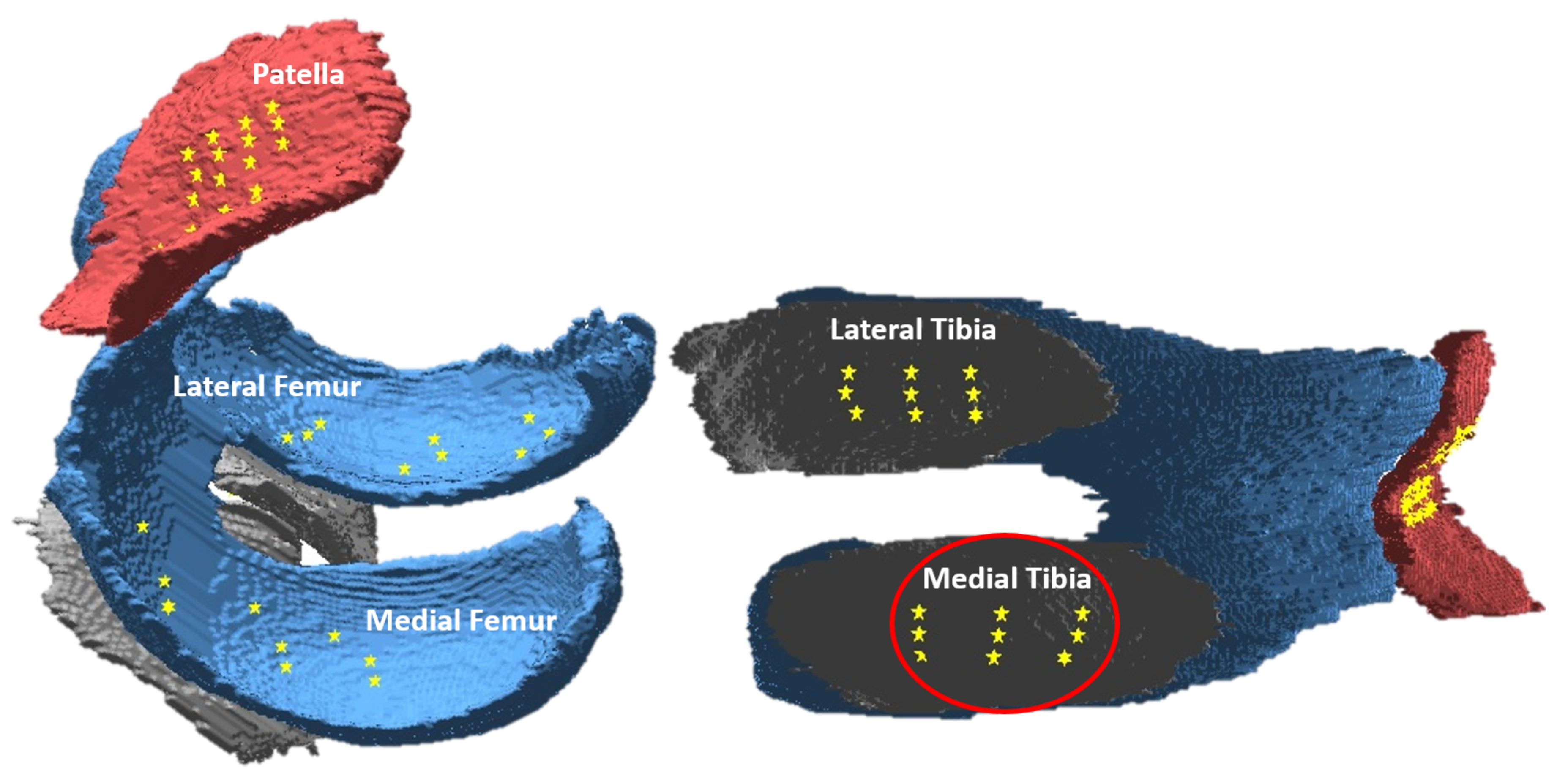
14] developed the cartilage damage index (CDI), which is an efficient and novel method for quantifying the cartilage volume. Instead of segmenting whole knee cartilage, this approach measures the thickness of the cartilage at certain informative locations (CDI locations) within the reconstructed cartilage layer. The selection of the informative locations is based on the statistical analysis that specific articular cartilage locations may experience more damage. When measuring CDI, a total of 60 locations within the cartilage layer are chosen, including nine locations from each of the four compartments (medial tibia, medial femur, lateral tibia, and lateral femur), and the rest 24 locations from the patella compartment as shown in
Figure 1. The CDI method has been tested and applied in several clinical trials supported by federal grants [
15]. The statistical analysis from those studies indicated that CDI is correlated with radiographic severity measures of the OA including Kellgren and Lawrence (KL) grade, Joint Space Width (JSW), Joint Space Narrowing (JSN), as well as knee alignment, all with
p-values less than 0.05 [
6,
14].
In this paper, we utilized the individual CDI locations identified in the work by the authors of [
14], to study the thickness change on cartilage. Additionally, we also employed manual segmentation as another channel to measure the thickness change. The difference is that CDI studies informative locations, while manual segmentation studies all the locations on the cartilage (all the cartilage points on the 2D slices). As a pilot study, we focused on the medial tibia compartment, since this compartment tends to have cartilage loss happen more frequently. Baseline and 12-month follow-up MR image data were used to extract cartilage thickness information from the medial tibia compartment. We tried to identify possible connections between the cartilage thickness information in the baseline year and the follow-up year. The artificial neural network (ANN) was employed to learn the changing pattern of cartilage thickness for both quantification methods.
The rest of the paper is organized as follows.
Section 2 provides a detailed description of the data and methods used in this study, including the OAI database, measurement of the CDI locations, whole cartilage segmentation, feature representation, ANN, and evaluation metrics.
Section 3 describes four groups of experiment which trained different ANN models for different feature sets. Results are presented and analyzed. Finally, the conclusion is drawn and future work is discussed in
Section 4.
2. Materials and Methods
2.1. Data
In order to promote the analysis of OA biomarkers as potential stand-in endpoints, National Institutes of Health and other partners created a large knee MRI image database called the Osteoarthritis Initiative (OAI) [
17]. The OAI data are collected from several clinical centers including Ohio State University, Brown University, University of Pittsburg, John’s Hopkins, and the University of Maryland. Approximately 4800 women and men in the age range between 45 and 79 years who were at a risk of knee OA were recruited in the five OAI clinical centers.
The research utilized a public labeled dataset, Imorphics, which is a subset from OAI, and composed of 81 pairs of knees (each pair contains the baseline and 12-month MR scans) [
18]. The 81 knees were selected from the OAI progression cohort, which included individuals with symptomatic knee OA in at least one knee. The baseline and 12-month follow-up images were manually segmented by experts and the raw data, including the manual segmentation, as well as the processed cartilage volume assessments are available through the OAI website [
19]. Additionally, all the knee joints in the dataset have complete data including semiquantitative radiographic grading, static knee alignment, and joint space width. The samples selected for the Imorphics dataset represented an even coverage of different OA severity levels (KL scores 0–4).
2.2. Cartilage Damage Index (CDI)
The CDI is a novel quantification approach for cartilage volume, which measures the volume through on 60 informative locations on the 3D MR images [
6,
14,
16]. The informative locations are mapped from various regions on the articular surface where denudation of the cartilage frequently happens. By using statistical analysis on hundreds of knees, 60 informative locations have been identified on 3D cartilage surface as indicated in
Figure 1. Then a customized software is used to locate and measure CDI points on the corresponding slice of the 3D MR image sequence. The software works as follows.
The initial step is to mark the most lateral and medial MR image slices that contain cartilage in the MR image sequence, which defines the range of the lateral-to-medial axis on the 2-dimensional coordinate system.
The software identifies the MR image slices that include CDI locations and measures the bone–cartilage boundaries.
It translates the bone–cartilage boundary length into a standardized anterior-to-posterior axis and pinpoints the nine informative locations that have been predefined.
It computes the cartilage volume score by adding up the product of voxel size, the cartilage thickness, and the cartilage length (anterior–posterior) from all the informative locations.
The software finally computes a total volume for each knee, but this study utilized the thickness information from individual CDI locations. We used the intermediate output of the software to study the cartilage changing pattern at the pixel level instead of as a whole.
2.3. Whole Cartilage Manual Segmentation
Three-dimensional (3D) MR images can be used to measure soft-tissue structures, including the intra-articular hyaline cartilage. A single 3D knee MR scan generates up to 160 2D slices in the sagittal view. On each slice, the boundary of knee cartilage can be manually delineated and the thickness information can be measured (number of pixels from each cartilage boundary position to its closest boundary position on the other side). However, the manual segmentation of the 3D sequence is quite time-consuming. It may take up to six hours to label one knee sequence with 160 images. For the Imorphics dataset used in this work, it took around one year for the experts to manually segment the cartilage of the 81 knees (81 × 160 = 12,960 images) [
18]. Additionally, the person who operates the segmentation software needs intensive training [
7], which also increases the cost of manual segmentation.
2.4. Feature Analysis
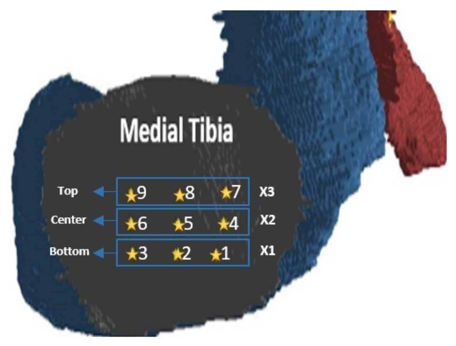
Different from previous studies, we did not study cartilage volume as a whole, instead, we treated the thickness information from each CDI informative location as an individual feature. Nine CDI locations on the medial tibia generated a 9-dimensional feature space (
Figure 2). These features provided input to the machine learning method ANN to predict if any thickness change occurred one year later. For each informative location, the thickness change over a year (subtracting baseline data from 12-month data) was computed to decide the output category. The corresponding class label was ’changed’ or ’no-change’. The label ’changed’ or ’no change’ is marked according to the difference of the thickness values between baseline year and 12-month follow-up year. In clinical studies, ’changed’ and ’no change’ represent a disease that has progression or no progression, which is an important sign to evaluate the effect of a treatment.
When using CDI, we compared the computed thickness values through CDI measurement at each of the nine locations. For example, for CDI position #1, if the baseline year thickness is 8, and the follow-up year thickness is 6, this position is marked as a ’changed’; if the absolute difference between the thickness values of the baseline and follow-up year is equal to 0 or 1, we mark the position as ’no-change’. These nine features were further divided into 3 groups; each group contained 3 CDI features from the top, center and bottom horizontal positions, respectively. As illustrated in
Figure 2, the top group contained CDI locations indexed 7, 8, and 9. The middle group contains the three CDI locations indexed 4, 5, and 6. The bottom group contained the CDI locations indexed 1, 2, and 3. We have trained separate ANN models for the combined nine CDI features as well as the three subgroups, respectively.
To obtain the features from manual segmentation, we first measured the thickness for each pixel along the cartilage boundary in one slice, and then saved the thickness values into a vector. In order to register different slices, we normalized thickness vectors into the universal length [1, 150]. The unified vectors represented the thickness information of baseline manual segmentation. In order to compare with the CDI features, we extracted the same three corresponding slices on the medial tibia that were used for CDI features, denoted by X1, X2, and X3 in
Figure 2. Our goal is to predict the thickness change at each pixel along the unified vector after 12 months, by using the baseline thickness information in the neighborhood as input features. In specific, for each pixel, we defined a mask including its left and right neighbors as the features for ANN; the output is ’changed’ or ’no change’ according to the difference between baseline and 12-month thickness vectors at this location. We mark ’no change’ if the absolute difference of thickness value between the baseline and the follow-up years is equal to 0 or 1 and ’changed’ otherwise.
2.5. Artificial Neural Network
Artificial neural networks (ANNs) are categorized as robust classifiers which are based on the functions and the structure of the biological neural networks [
20]. In this study, we used ANN to model the changing pattern of the cartilage thickness. ANNs are composed of an input layer, one or more hidden layers, and an output layer. The network structure in this study was composed of a single hidden layer that had n neurons, whereby n is calculated as number_of_attributes + number_of _classes and then divided by 2. The weight of the neurons was updated using the backpropagation algorithm. We implemented ANN by using the Weka software package [
21].
2.6. Evaluation
The 70/30 random separation was used to separate training and testing data. Eighty-one knees were subdivided randomly into training and testing sets, i.e., the training set contained 57 knees while the testing set contained 24 knees. Note that the separation was done manually at the knee level, not at the image level, to guarantee that the images from the same knee will not exist in both training and testing.The reason we used 70/30 random separation instead of running the cross-validation is that our dataset is large enough (which contains 4941 slices) to test if the changing pattern of cartilage is predicable.
We adopted multiple metrics to evaluate the performance of our prediction models. These metrics include Mathew’s correlation coefficient (MCC), the F-measure, recall (also known as sensitivity), precision (also regarded as the positive predictive value (PPV)), and area under the receiver operating characteristic (ROC) curve (AUC). The MCC provides a powerful evaluation of accuracy within the machine learning approaches especially in the case where the number of negative and positive samples is not balanced. The F-measure depicts the overall accuracy of the classification as a weighted average for recall and precision for a specific confidence threshold. The area under ROC curve (AUC) provides a comprehensive evaluation of the classifier as the trade-off between true positive rate and false positive rate is adjusted. Below are the formulas for the evaluation metrics.
In this study, the “positive” case is defined as the change (actually loss) of the cartilage since a gradual loss of cartilage is an important sign of knee osteoarthritis. Correspondingly, no change of cartilage is a “negative” sign. To label if there is a real change, i.e., ground truth, we need to measure the thickness of each cartilage position in the baseline and follow-up years. Here we consider manual segmentation and CDI as two different ways to measure the thickness of cartilage and aim to compare which way is more reliable and applicable to track the change of cartilage.
Based on the above definitions of positive and negative, TN (true negative) is defined as a position where thickness does not change within the 12 months, and the ANN model predicts so. TP (true positive) is defined as a position where the thickness value changes within the 12 months and the ANN model predicts so. Correspondingly, FP (false positive) is defined as there is no change in the thickness within the 12 months but the ANN predicts that there is a change, and FN (false negative) is defined as there is a change in the thickness within the 12 months but the ANN predicts that there is no change for that position.
3. Experiment and Results
The purpose of this work is to explore if any detectable pattern exists to model knee cartilage change. We used ANNs and two cartilage quantification methods to explore the pattern. We started from building separate models for different cartilage locations, and finally trained one model for the whole cartilage. The reason for doing so was based on the clinical observation that cartilage loss tends to happen at certain weight-bearing regions, and therefore different locations might present different patterns.
3.1. Experiment 1: Cartilage Change Prediction at the Bottom Horizontal Line
Experiment 1 was designed to study the changing pattern of cartilage at the lower position of the medial tibia compartment. When we chose CDI as the quantification method, CDI points (# 1, #2, and #3 in
Figure 2) were used to represent cartilage thickness; when we chose manual segmentation to quantify cartilage volume, we used X1 slice (see
Figure 2) at the bottom horizontal line to represent cartilage thickness information.
We first described the feature space for CDI. For each CDI location, we used the thickness values of the baseline year at the location itself as well as its two neighbors, forming a 3-dimensional feature vector as an input to the ANN, to predict ’changed’ or ’no change’ class label. Specifically, to predict change at CDI # 2, we used CDI values at locations #1, #2, and #3 to form the feature vector. To predict change at CDI #1, we used #2, #1, and #2 to form the feature vector, by a mirror padding at the right side of #1. The same procedure was implemented to generate the feature vector for CDI location #3. The output is ’changed’ if there is a change of thickness value at that CDI location at 12-month follow-up and ’no-change’ otherwise, indicating the OA disease has ’progression’ or ’no progression’. In terms of the manual segmentation to quantify cartilage thickness, for each pixel, similarly, we have a neighborhood thickness vector as input and ’changed’ and ’no-change’ as output. To match the CDI method, we found the corresponding MR slice (such as X1 in
Figure 2) that contained the corresponding CDI locations. Unlike CDI using only three locations on one MR slice, all the locations along the cartilage layer on the MR slice were included in the analysis when using manual segmentation to quantify the cartilage. Take X1 slice for example, a thickness vector was obtained to represent the thickness value of each pixel along with cartilage on X1 slice. We treated every single pixel as a sample and used the thickness of itself and its surrounding neighborhood pixels to predict the change of thickness at this particular position one year later. We tested various sizes of neighborhood including three neighbors (the pixel itself plus immediate left and right pixels) to 149 neighbors (the pixel itself plus 74 pixels on the left and 74 pixels on right) to find the best prediction performance using manual segmentation. The best AUC of ANN was using 75 neighbors (37 left and 37 right, mirror padding for pixels near the two ends).
The general methodology to study the manual segmentation and CDI is the same, i.e., they both use neighborhood thickness vector as input to ANN, and use ’changed’ or ’no-change’ as output for each sample pixel. The difference is at the input dimension for each sample and the number of samples. The manual segmentation has a much larger sample pool since every pixel along the cartilage boundary is considered as a sample while the CDI has limited sample locations. This is the potential advantage of CDI that we only need to measure a few representative locations, but we can still, or even better, track the change of cartilage.
We used the same training and testing data separation (as discussed in
Section 2.6) for the two quantification methods. Because we noticed the data distribution had severed unbalance between ’changed’ and ’no-change’ categories (much more ’no-change’ than ’changed’), we conducted resampling on the training dataset to balance the two categories.
Table 1 shows the distribution of the two categories on the original dataset and rebalanced dataset. The performance of ANN model on both datasets was summarized in
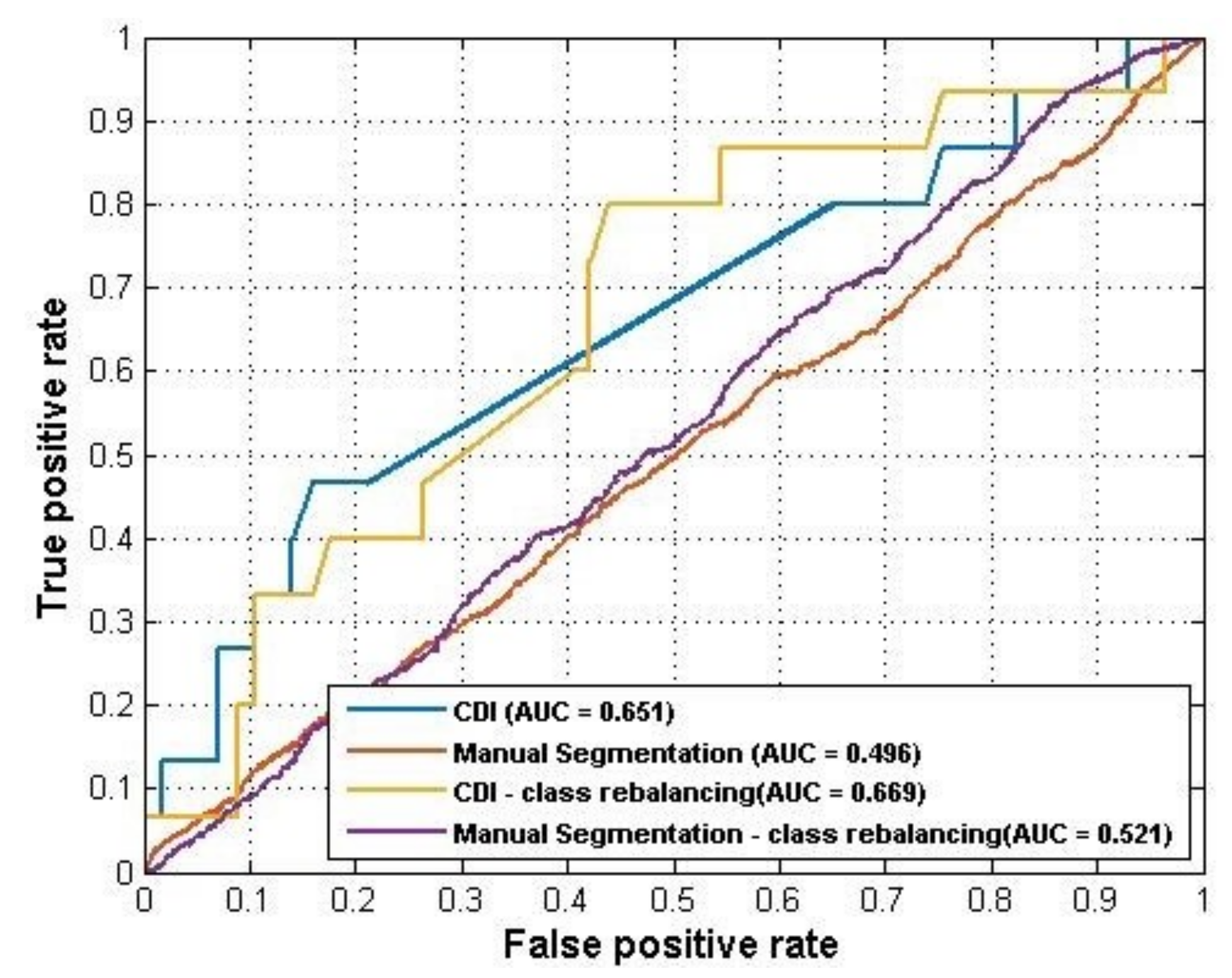
Table 2. As the results showed, the CDI generated a better performance (AUC = 0.651) than manual segmentation (AUC = 0.496) using raw data. For the rebalanced dataset, the CDI also showed a better prediction performance than manual segmentation (AUC = 0.669 VS AUC = 0.521). The ROC curves of these four ANN models were plotted in
Figure 3.
Note that different rebalance strategies were applied to the training set of the CDI and manual segmentation data, due to the difference in sizes. For the CDI, the synthetic minority oversampling technique (SMOTE) [
22] was applied. SMOTE is an oversampling technique that generates more samples for the minority class. The new samples are not just copies of existing minority cases; instead, the algorithm combines the features of the target case with the features of its neighbors. Since only nine CDI locations were used to generate samples for each knee case, the dataset size was relatively small. Using SMOTE can increase the training data size and make samples more general. To rebalance the classes for manual segmentation, an undersampling strategy was applied to the training set which reduced the majority class. This was because the original dataset was already very large (since every pixel along the cartilage was used as a sample). After dataset rebalances, the performance of both models improved. The AUC of the CDI method improved from 0.651 to 0.669 while the AUC of manual segmentation was improved from 0.496 to 0.523.
3.2. Experiment 2: Cartilage Change Prediction at the Middle Horizontal Line
A parallel experiment was conducted to detect the changing pattern of cartilage at the middle horizontal line on the medial tibia compartment (see
Figure 2). For CDI, the three center locations (#4, #5, and #6) were used to extract thickness information, and for manual segmentation, the X2 slice was used. We performed the same rebalance operations as used in experiment 1.
Table 3 listed the distribution of the ’change’ and ’no-change’ categories for experiment 2.
As
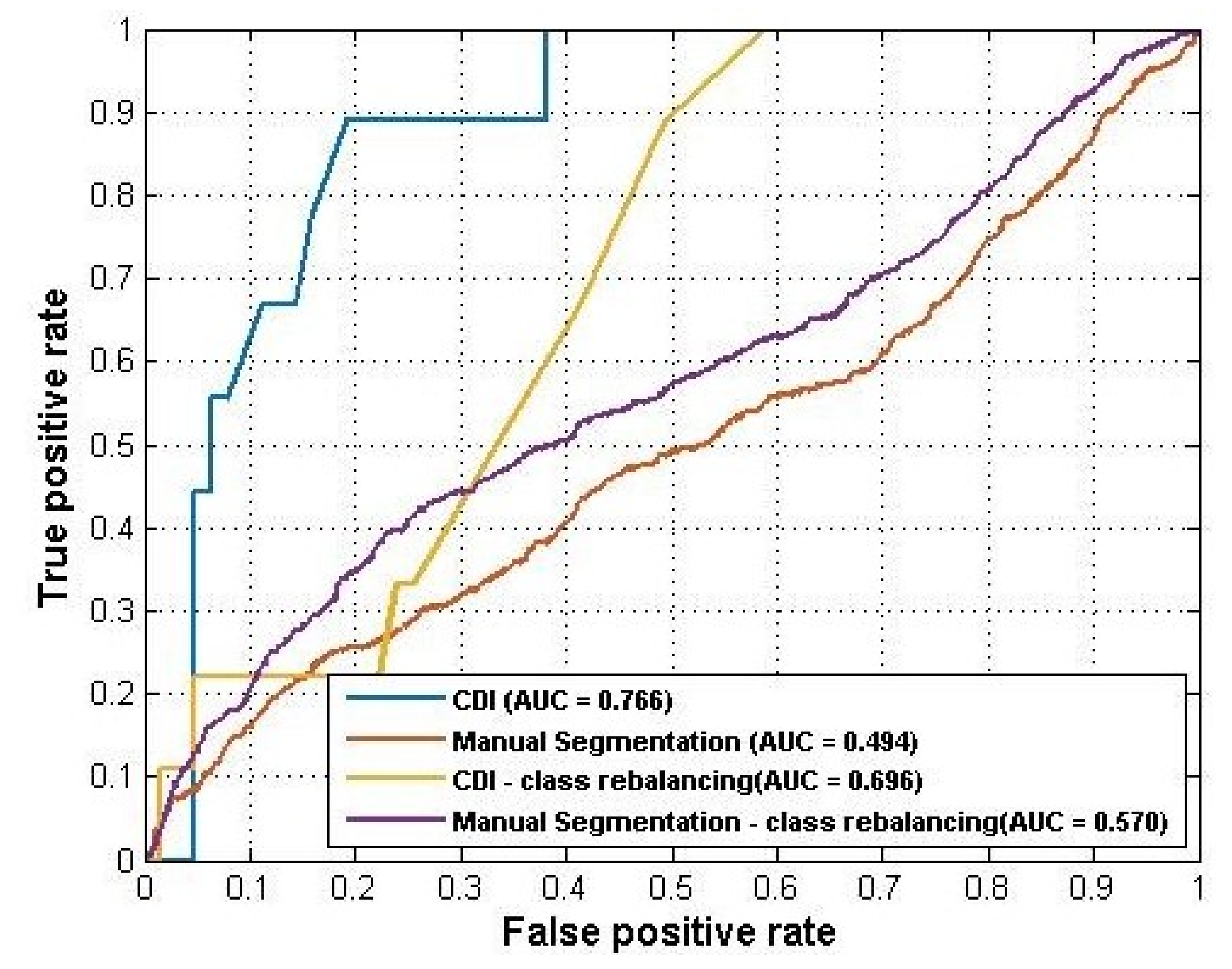
Table 4 showed, the CDI method outperformed manual segmentation and achieved AUC = 0.766 and F-measure = 0.839. Additionally, the oversampling did not help the CDI improve its performance in this experiment while the undersampling improved the AUC of the manual segmentation from 0.494 to 0.524. Overall, the CDI still outperformed manual segmentation significantly on predicting cartilage change in the middle slice of the medial tibia compartment.
Figure 4 showed the ROC curves for these models.
3.3. Experiment 3: Cartilage Change Prediction at the Top Horizontal Line
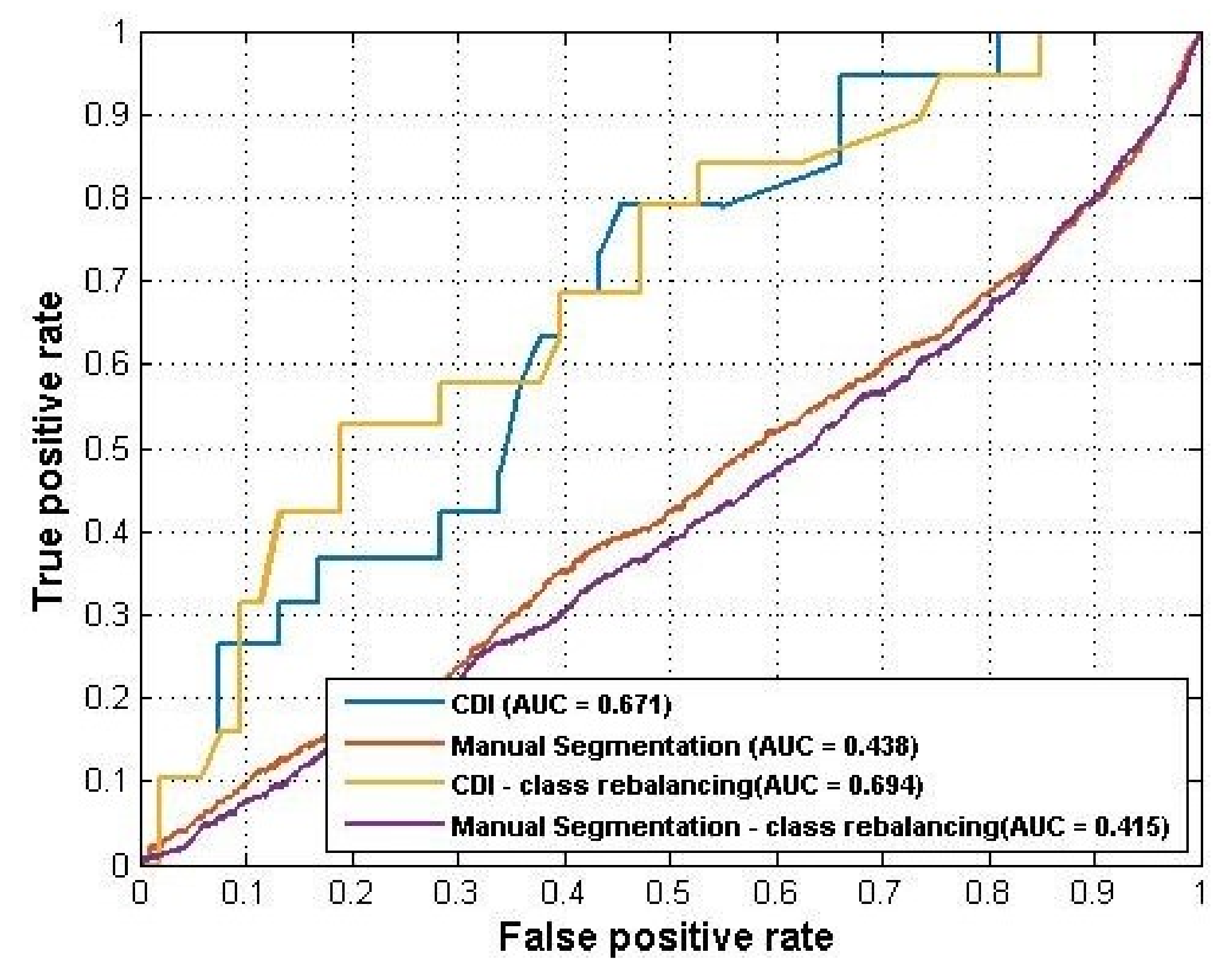
This experiment trained models using the top three CDI locations (#7, #8, and #9) and slice X3 for manual segmentation to predict the change of cartilage.
Table 5 listed the distribution of the ’change’ and ’no-change’ categories.
Table 6 summarized the results and
Figure 5 plotted the ROC curves.
Again, the CDI generated better performance (AUC = 0.671) than manual segmentation (AUC = 0.438). For this experiment, the sample rebalancing strategies helped improve the performance of CDI but did not affect the performance of manual segmentation by much.
3.4. Experiment 4: Whole Medial Tibia Cartilage Prediction
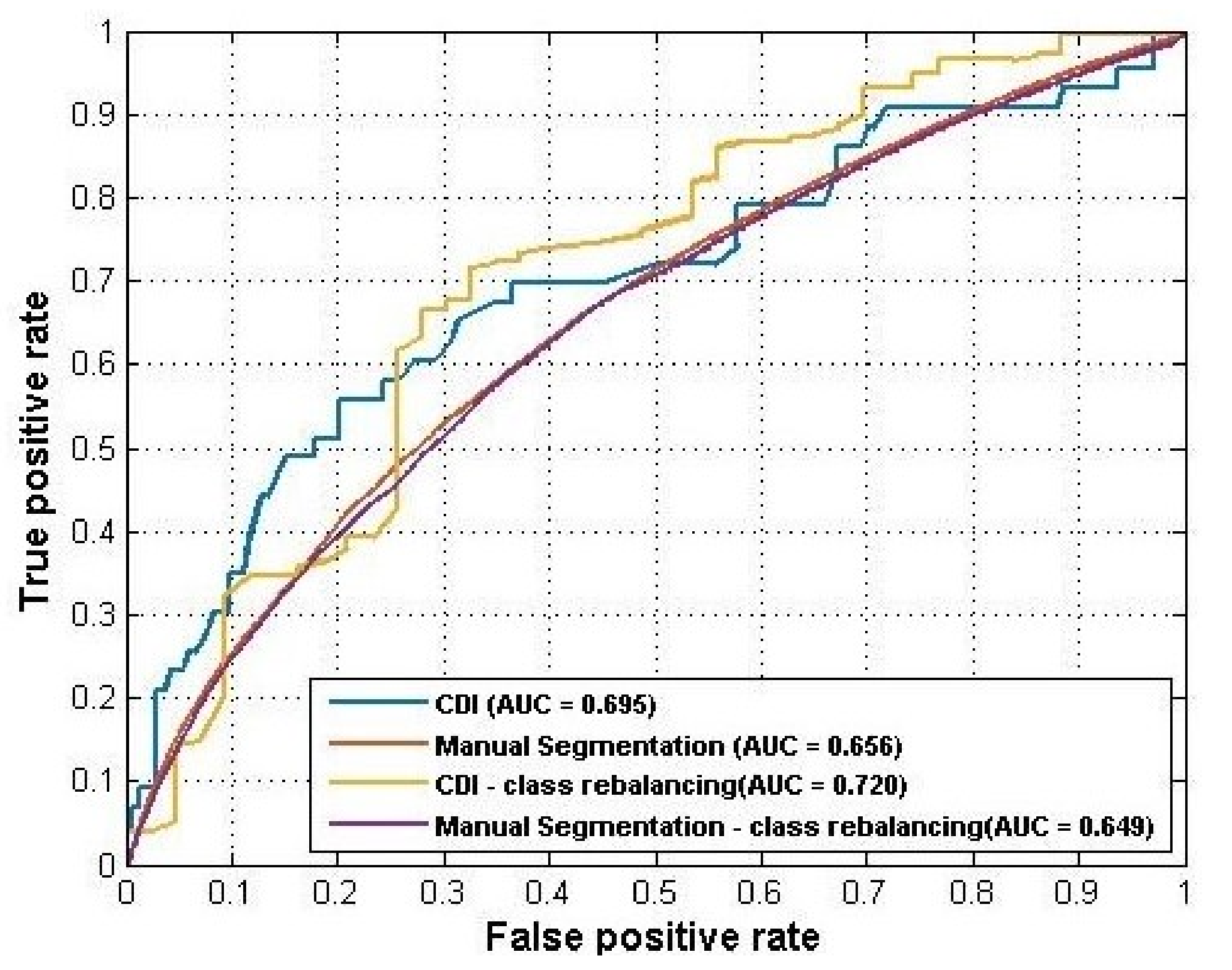
In this experiment, we combined the feature space of the three experiments above to train a single model for the whole medial tibia compartment. For CDI, all the nine CDI locations were included and for manual segmentation, all locations from the three slices were used to generate samples.
Table 7 listed the distribution of the ’change’ and ’no-change’ categories for the whole dataset.
Table 8 summarized the prediction performance and
Figure 6 plotted the ROC curves of the four models. CDI still achieved better performance than manual segmentation in both the raw dataset and the rebalanced dataset. Rebalancing strategies helped improve the performance of CDI to AUC = 0.720 but did not help the manual segmentation.
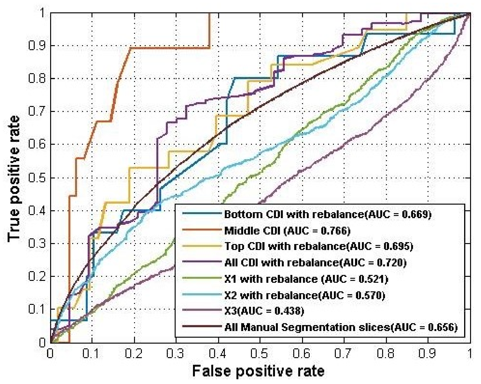
In addition, we compared the four groups of experiments longitudinally. Such a comparison gave us a better idea of how different feature spaces performed using the same quantification method. The best performance from the above four groups of the experiment was summarized into
Table 9. For CDI, the central CDI locations achieved the best AUC = 0.766 on the rebalanced dataset, which indicated that the pattern of cartilage changing was stronger in the central region of medial tibia compartment. For manual segmentation, the combination of all slices of a knee MR sequence generated the best AUC = 0.656 than using only the individual slice. Overall, using CDI identifies a stronger pattern of cartilage change than using manual segmentation, no matter employing subregion features or the whole feature space.
Figure 7 plotted the ROC curves of the models using different feature spaces.
Finally, we compared the performance of ANN with a simple baseline classifier (ZeroR) using whole medial tibia data. ZeroR [
23] is the simplest classification method which relies on predicting the majority class while ignoring the other class on the binary problem. Despite the fact that there is no predictability power in ZeroR, it is helpful for deciding a baseline performance on the imbalanced classification problems and compare its performance with our classification method. The performance of ZeroR was same before and after using rebalance.
Table 10 compared the performance of the two classifiers and as the results showed, ANN significantly outperformed the baseline classifier.
4. Discussion and Conclusions
In this work, we launched a pilot study to explore the changing pattern of knee cartilage using ANN and two different quantification methods. The manual segmentation method takes more time to quantify a 3D knee MR sequence while the CDI is much faster because it selects only a few informative locations rather than measures the whole cartilage. Using the Imorphics dataset with 81 knees, we compared the prediction accuracy of cartilage change using the two quantification methods and found that the CDI generated better performance in predicting the change of cartilage thickness in a 12-month period.
There are two interesting findings in our study: (1) The central horizontal line generated the best prediction performance compared to the other CDI locations, which indicated that the central region may have clearer and stronger changing patterns than other regions. This reflects the fact that central cartilage regions usually bear more body weight. Therefore, more attention should be paid to the central region when selecting more CDI points. (2) In terms of predicting cartilage thickness change, the easier and faster quantification method CDI generated higher accuracy than manual segmentation (0.720 vs. 0.656 for all slides). The accuracy is not high for both methods and there is still space for improvement.
One of our future work is to extend the current study to other knee compartments, including the lateral tibia, femur, and patella. Trying different machine learning methods (other than ANN) is another interesting direction. In addition, we will extend our dataset to incorporate more cases from the OAI database. This will help explore more useful information from the data and obtain a better understanding of knee OA disease.


