Bidirectional Long Short-Term Memory Neural Networks for Linear Sum Assignment Problems

Abstract

Many resource allocation problems can be modeled as a linear sum assignment problem (LSAP) in wireless communications. Deep learning techniques such as the fully-connected neural network and convolutional neural network have been used to solve the LSAP. We herein propose a new deep learning model based on the bidirectional long short-term memory (BDLSTM) structure for the LSAP. In the proposed method, the LSAP is divided into sequential sub-assignment problems, and BDLSTM extracts the features from sequential data. Simulation results indicate that the proposed BDLSTM is more memory efficient and achieves a higher accuracy than conventional techniques.

1. Introduction

The linear sum assignment problem (LSAP) is a special case of the linear programming problem that aims to minimize the cost of assigning multiple tasks to a number of agents on a one-to-one basis. In wireless communications, many resource allocation tasks can be modeled as the LSAP, such as joint relay selection and resource allocation for device-to-device communications [1], joint resource allocation with multi-cell cooperation in virtual multiple-input multiple-output (MIMO) systems [2], and unlicensed channel allocation for LTE systems [3].

For LSAPs, the Hungarian algorithm has been proposed to obtain the optimal solution without an exhaustive search [4]. Furthermore, heuristic algorithms such as deep greedy switching [5], the interior point [6], or the dual forest algorithm [7] have been investigated to estimate near-optimal solutions in real-world problems with time constraints.

In recent years, deep neural networks (DNNs) have recently achieved state-of-the-art performance in different fields such as audio processing [8,9], visual object recognition [10], and other domains [11,12,13]. Neural networks (NNs) can extract features from input implicitly and approximate an arbitrary math function. Several approaches have applied DNNs to solve mathematical optimization problems [14,15]. In [2], a DNN was used to approximate an optimization algorithm in interference management. In [16], an LSAP was decomposed into several sub-assignment problems and two types of DNNs, i.e., the feed-forward neural network (FNN) and convolutional neural network (CNN) [17] were applied to address sub-assignment problems. However, the DNNs discussed in [16] have not achieved much success owing to the increasing size of the problem.

Hence, a bidirectional long short-term memory neural network (BDLSTM) is proposed to solve LSAPs. In the proposed method, an LSAP is decomposed into a sequence of smaller sub-assignment tasks that become the model input, in which each layer consists of two separated smaller LSTM layers. The intermediate outputs of these layers are combined to process data in both the forward and backward directions. The BDLSTM structure is better at remembering the LSAP than other structures by combining the hidden layer outputs of each sub-assignment problem together. Finally, a collision-avoidance algorithm is applied to the output to obtain the final result. Simulation results indicate that the proposed BDLSTM outperforms the FNN and CNN models when the size of the problem increases, while requiring less parameters to model the patterns.

2. Preliminary

2.1. Problem Formulation

In LSAPs [4], given a set of n jobs $I=\{1,\dots ,n\}$ and n agents $J=\{1,\dots ,n\}$, we wish to minimize the cost of assigning each job to each agent. Assigning job i to agent j results in a cost value of $U_{ij}$, and the problem can be formulated as follows:

$$min\sum _{i=1}^n\sum _{j=1}^n{u}_{ij}{x}_{ij},$$

(1)

subject to:

$$\sum _{i=1}^n{x}_{ij}=1,j=1,\dots ,n,$$

(2)

$$\sum _{j=1}^n{x}_{ij}=1,i=1,\dots ,n,$$

(3)

$$x_{ij}\in \{0,1\},i,j=1,\dots ,n,$$

(4)

where $x_{ij}$ is the decision indicator value. $x_{ij}=1$ when job i is assigned to agent j; otherwise, $x_{ij}=0$. We can rewrite the cost values as an n by n matrix $\mathbf{U}={[{\mathbf{u}}_1,\dots ,{\mathbf{u}}_n]}^T$ and decision indicator values as an n by n permutation matrix $\mathbf{X}={[{\mathbf{x}}_1,\dots ,{\mathbf{x}}_n]}^T$, where ${\mathbf{u}}_i={[u_{i1},\dots ,u_{in}]}^T$ and ${\mathbf{x}}_i={[x_{i1},\dots ,x_{in}]}^T$. In the communication field, many optimization problems are similar or can be formulated as LSAP [1,2,3].

In [16], the LSAP problem was firstly decomposed into multiple sub-assignment problems to implement DNNs. However, the DNNs in [16] did not address the sequential information in the cost matrix, as multiple FNN and CNN models must be applied to solve all sub-assignment problems simultaneously. Here, a single neural network model is considered to extract the necessary features to solve LSAPs.

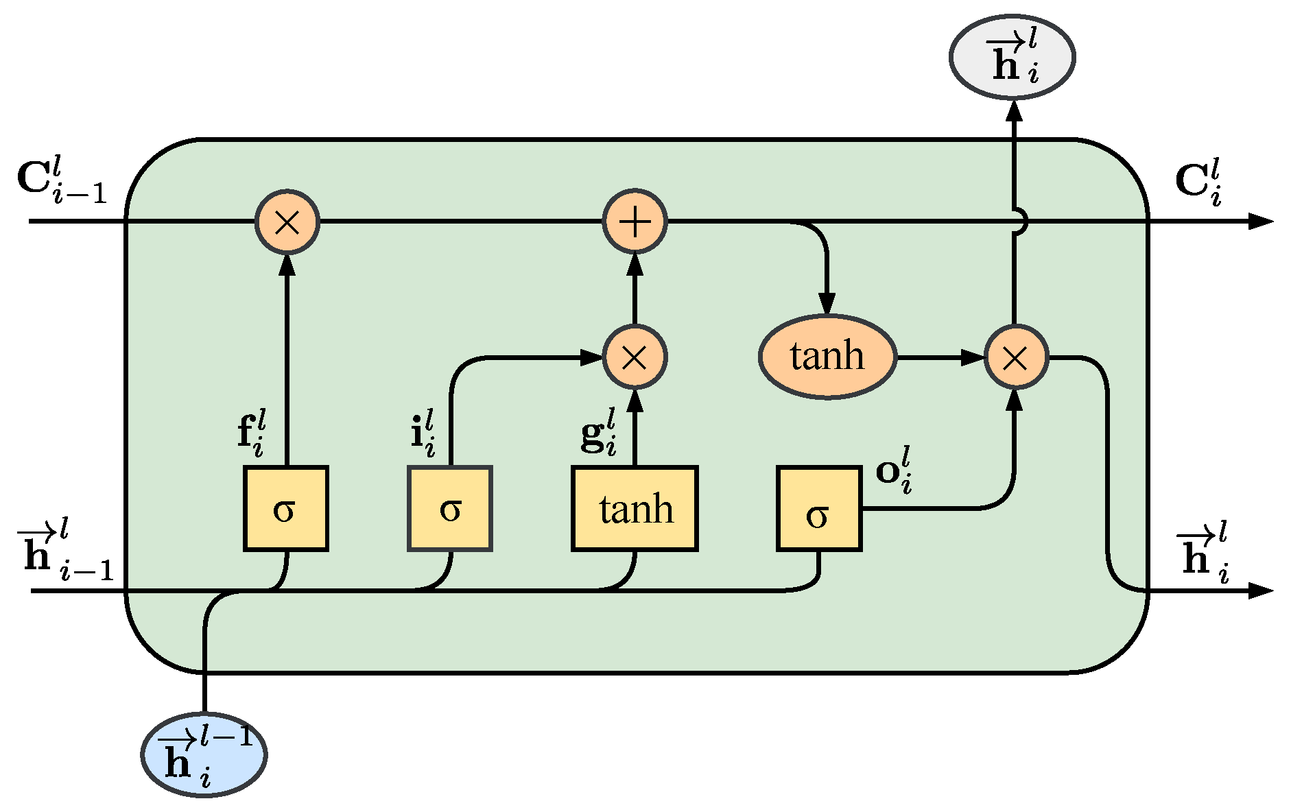
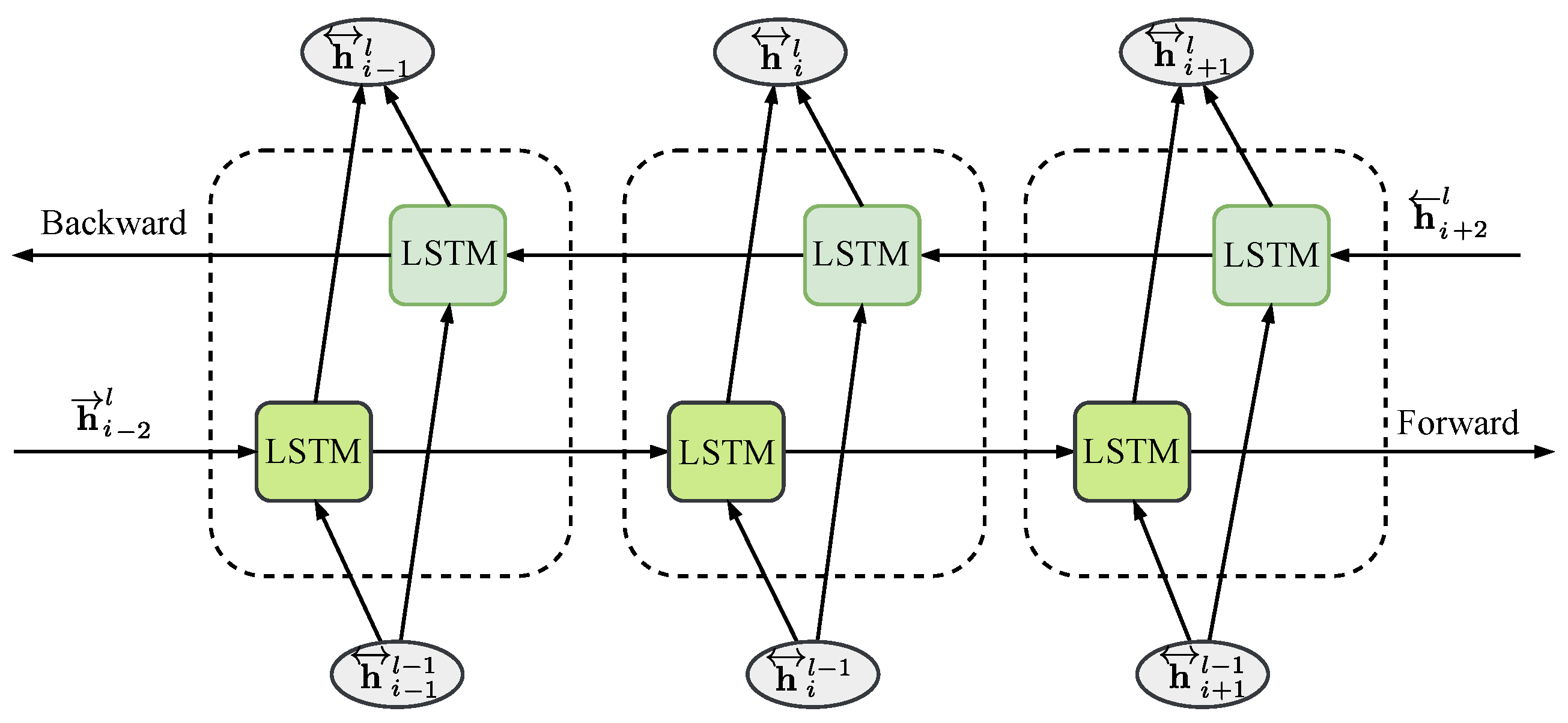
2.2. Bidirectional LSTM

The structure of a conventional LSTM model is illustrated in Figure 1. Here, we provide a short introduction to the LSTM model. For further details, we refer the interested reader to [18]. LSTM [18] was designed with special memory cells to store temporal information. This structure allows LSTM to remember long-range features better than conventional recurrent neural networks. With a multilayer model, components of a cell at time step i at layer l in the forward direction can be implemented by the following functions:

$${\mathbf{f}}_i^l=\sigma \left({\mathbf{W}}_{\left(f\right)}^l{\overrightarrow{\mathbf{h}}}_i^{l-1}+{\mathbf{V}}_{\left(f\right)}^l{\overrightarrow{\mathbf{h}}}_{i-1}^l+{\mathbf{b}}_{\left(f\right)}^l\right),$$

(5)

$${\mathbf{i}}_i^l=\sigma \left({\mathbf{W}}_{\left(i\right)}^l{\overrightarrow{\mathbf{h}}}_i^{l-1}+{\mathbf{V}}_{\left(i\right)}^l{\overrightarrow{\mathbf{h}}}_{i-1}^l+{\mathbf{b}}_{\left(i\right)}^l\right),$$

(6)

$${\mathbf{o}}_i^l=\sigma \left({\mathbf{W}}_{\left(o\right)}^l{\overrightarrow{\mathbf{h}}}_i^{l-1}+{\mathbf{V}}_{\left(o\right)}^l{\overrightarrow{\mathbf{h}}}_{i-1}^l+{\mathbf{b}}_{\left(o\right)}^l\right),$$

(7)

$${\mathbf{g}}_i^l=\tanh \left({\mathbf{W}}_{\left(g\right)}^l{\overrightarrow{\mathbf{h}}}_i^{l-1}+{\mathbf{V}}_{\left(g\right)}^l{\overrightarrow{\mathbf{h}}}_{i-1}^l+{\mathbf{b}}_{\left(g\right)}^l\right),$$

(8)

$${\mathbf{C}}_i^l={\mathbf{f}}_i^l\odot {\mathbf{C}}_{i-1}^l+{\mathbf{i}}_i^l\odot {\mathbf{g}}_i^l,$$

(9)

$${\overrightarrow{\mathbf{h}}}_i^l={\mathbf{o}}_i^l\odot \tanh \left({\mathbf{C}}_i^l\right),$$

(10)

where ${\mathbf{i}}_i^l$, ${\mathbf{f}}_i^l$, ${\mathbf{o}}_i^l$, ${\mathbf{g}}_i^l$, ${\mathbf{C}}_i^l$, and ${\overrightarrow{\mathbf{h}}}_i^l$ are the input gate, forget gate, output gate, candidate gate, cell state, and hidden state, respectively, all of which are of the size of an $N^l$-dimensional vector. In (6)–(9), the ${\mathbf{W}}^l$ terms are the weight matrices between cells of layer $(l-1)$–l, the ${\mathbf{V}}^l$ terms are the weight matrices between consecutive cells of layer l, and the ${\mathbf{b}}^l$ terms are the bias vector at each layer. The weight matrices and bias values in a cell are shared along the length of the sequence, thus reducing the total number of weights and hidden neurons in the network. The sigmoid function $\sigma$ and hyperbolic tangent function are used as activation functions, and ⊙ denote element-wise multiplication.

A bidirectional LSTM can process the data in both the forward and backward directions using two separate LSTM layers. The forward hidden state, ${\overrightarrow{\mathbf{h}}}_i^l$, calculated by the formulas above, and the backward state, ${\overleftarrow{\mathbf{h}}}_i^l$, calculated similarly, are concatenated and then fed forward to the next layer, as demonstrated in Figure 2:

$$\overleftrightarrow{{\mathbf{h}}_i^l}=\left[\begin{array}{c}{\overrightarrow{\mathbf{h}}}_i^l\\ {\overleftarrow{\mathbf{h}}}_i^l\end{array}\right],$$

(11)

where $l=0$ is the input layer. BDLSTM is better at obtaining the relations among elements in a whole sequence by utilizing information in both directions, instead of remembering the features in only one direction such as that of the conventional LSTM. Furthermore, by using the parameter-sharing technique in a layer, the BDLSTM model requires less memory to solve the problem compared to the conventional FNN and CNN.

3. Proposed Method

This section presents the proposed BDLSTM model for LSAPs. The architecture and details of the proposed model are elaborated in Section 3.1. In Section 3.2, the training process is explained.

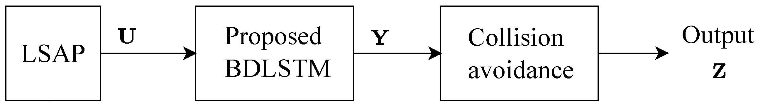
3.1. System Model

Figure 3 shows the proposed system architecture for solving an LSAP. A deep-learning-based BDLSTM model is first applied to the cost matrix of the LSAP. After that, a collision-avoidance algorithm is applied to solve any interference in the outputs of the proposed BDLSTM model. In the proposed BDLSTM model, the constraint in (3) is not taken into consideration, which guarantees that one job can be assigned to only one agent. This is because the proposed BDLSTM model solves each sub-assignment task as a separate classification problem. The collision-avoidance algorithm prevents one job from being assigned to multiple agents simultaneously.

As described in Figure 4, in the proposed BDLSTM model, the cost matrix $\mathbf{U}$ is divided into n sub-assignment tasks ${\mathbf{u}}_i$, where $i=1,\dots ,n$ and ${\mathbf{u}}_i$ is the cost vector for job i. The ${\mathbf{u}}_i$ are used as the input sequence of the BDLSTM model as ${\overrightarrow{\mathbf{h}}}_i^0={\overleftarrow{\mathbf{h}}}_i^0={\mathbf{u}}_i$. After L consecutive BDLSTM layers to extract the features, all hidden states at the last layer ${\overleftrightarrow{\mathbf{h}}}_i^L$ will be applied in an identical fully-connected layer with the softmax activation function to obtain the output matrix $\mathbf{Y}={[{\mathbf{y}}_1,\dots ,{\mathbf{y}}_n]}^T$:

$${\mathbf{y}}_i=\mathrm{softmax}({\mathbf{W}}_y{\overleftrightarrow{\mathbf{h}}}_i^l+{\mathbf{b}}_y),$$

(12)

where ${\mathbf{W}}_y$ and ${\mathbf{b}}_y$ are the weight matrix and bias of the output layer, respectively. After the BDLSTM model, a decision matrix can be obtained by $\overline{\mathbf{Y}}={\left[{\overline{\mathbf{y}}}_1,\dots ,{\overline{\mathbf{y}}}_n\right]}^T$, where ${\overline{\mathbf{y}}}_i$ is obtained by one-hot encoding of ${\mathbf{y}}_i$. In collision avoidance, the collision cases in $\overline{\mathbf{Y}}$ are corrected using the Hungarian algorithm by the following steps:

• Step 1: Find jobs that are assigned to multiple or no agents.
• Step 2: Extract the cost values of jobs from Step 1 as a small LSAP.
• Step 3: Solve the LSAP from Step 2 using the Hungarian algorithm.
• Step 4: $\overline{\mathbf{Y}}$ is modified into a decision matrix $\mathbf{Z}$ using Step 3, where $\mathbf{Z}$ is an n by n permutation matrix.

For sequential data, FNNs, CNNs, and especially recurrent structures such as LSTM and BDLSTM are widely used and have achieved many successes. FNNs can be applied to every problem as the baseline architectures. CNNs are more complicated and have good performance in computer vision and some natural language processing tasks. On the other hand, LSTMs and BDLSTMs are recurrent structures built specifically for problems relating to sequential data. In the proposed method, BDLSTM is used to extract the features from the cost matrix $\mathbf{C}$, and each classification is based on the information of the whole cost matrix. Compared to the FNN and CNN in [16], BDLSTM has memory cells, which can remember the relationship between the cost vectors of consecutive sub-assignment tasks.

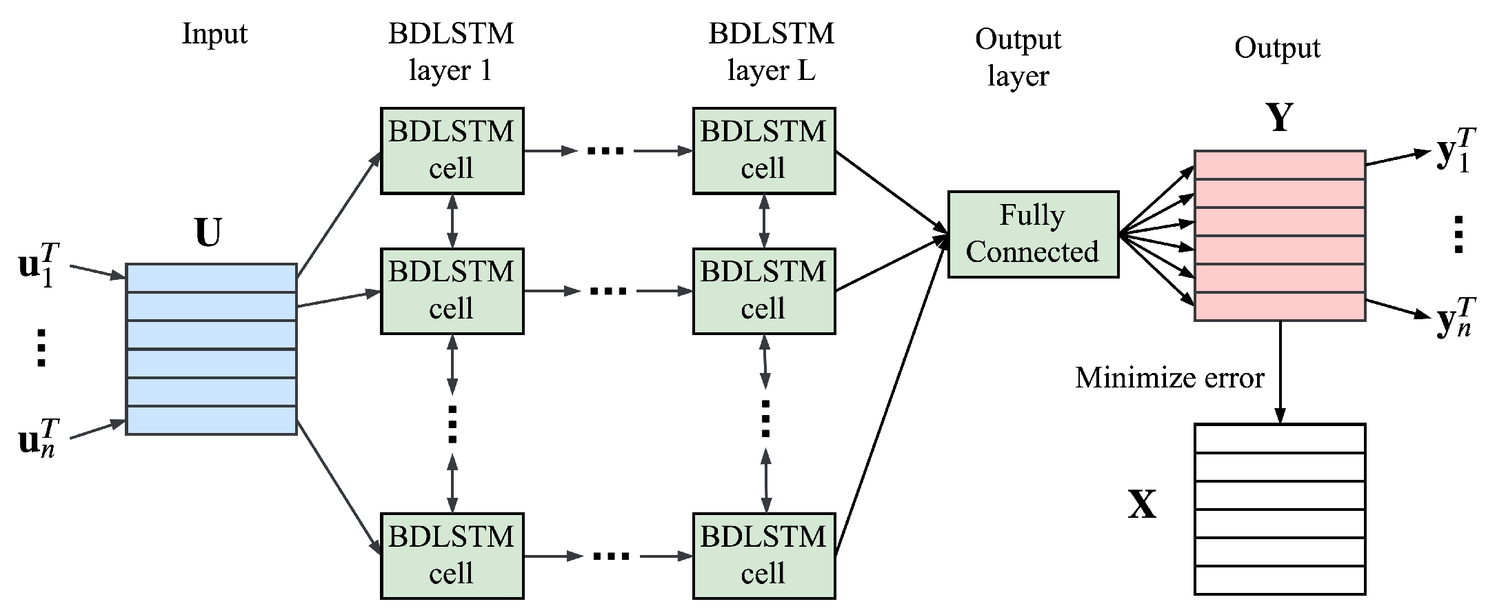
3.2. Training Stage

The training dataset consists of M data entries, each of which is a pair of cost and decision matrices $\{\mathbf{U},\mathbf{X}\}$. First, we generate the cost matrix $\mathbf{U}$, where each cost value $u_{ij}$ is a real value and is generated from a uniform distribution on (0, 1]. Then, the optimal decision matrix $\mathbf{X}$ according to $\mathbf{U}$ is obtained for the training dataset using the Hungarian algorithm [4]. After repeating this step M times, we can generate the whole dataset. For this experiment, we used $M=500,000$ samples. Among these, 10% of this dataset was sampled randomly for validation at the end of each training epoch to select the hyperparameters while preventing the overfitting problem. After completing the training step, 50,000 unseen samples were used as the test dataset to verify the performance of the trained model.

In the training process, the mini-batch gradient descent procedure was applied to optimize the parameters of the models to minimize the following total loss:

$$Loss=\frac{1}{\left|\mathcal{B}\right|}\sum _{m\in \mathcal{B}}\mathcal{L}\left(m\right),$$

(13)

where $\mathcal{B}$ is a minibatch sampled from the dataset with size $\left|\mathcal{B}\right|$ and $\mathcal{L}\left(m\right)$ is the loss computed from samples $m\in \mathcal{B}$. For this classification task, we chose the cross-entropy as the loss function, which can be formulated as follows:

$$\mathcal{L}\left(m\right)=-\sum _{i=1}^n{\mathbf{x}}_i^{\left(m\right)}\odot log\left({\mathbf{y}}_i^{\left(m\right)}\right).$$

(14)

The weights were updated based on the gradient information of the loss function. We chose the Adam algorithm [19] as the gradient descent method as it required only the first-order gradient to be computed, thus reducing the calculation complexity.

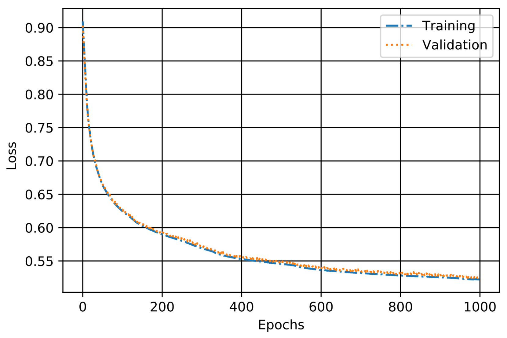
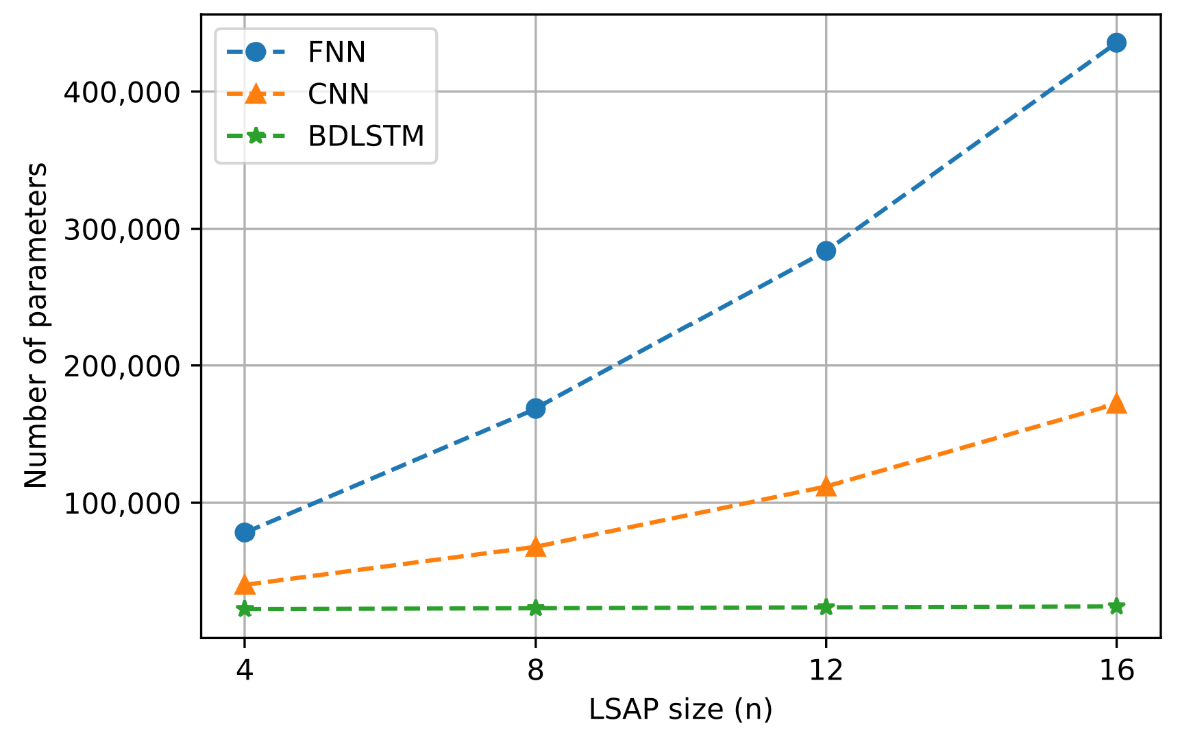
4. Performance Evaluation

In this section, we evaluate the simulation results of the proposed scheme using a BDLSTM model with different configurations for the LSAP. To obtain the optimized hyper-parameters, such as batch size, number of epochs, and learning rate, the proposed model was trained using several combinations of parameters using grid search, and the best combination was selected. The BDLSTM model with $L=4$ layers was chosen, and each layer contained $N^l=16$ hidden units at each gate.

Figure 5 shows the convergence of the BDLSTM over each training epoch on the training and validation set with $n=16$ and a batch size $\left|\mathcal{B}\right|=1024$. The loss of the model on both datasets decreased steadily after each epoch, and the gap was minimal, suggesting no overfitting during training.

Table 1. Accuracy performance comparison.

	$\mathit{n}=4$	$\mathit{n}=8$	$\mathit{n}=12$	$\mathit{n}=16$
FNN [16]	97.63	70.19	59.18	56.14
CNN [16]	98.29	82.95	66.05	62.74
LSTM	77.15	67.82	64.20	60.35
BDLSTM	98.85	94.47	86.54	78.82

shows the accuracy performance comparisons between the proposed BDLSTM model and other neural network structures, where the FNN and CNN were based on [16], and a uni-directional LSTM model was used with the same number of layers and hidden units for the proposed model. The FNN consisted of n smaller models, each having four layers with 32, 64, 256, and n hidden neurons. The CNN consisted of five convolutional layers, each containing 32, 32, 32, 32, and n kernels, and n output layers, each with n neurons. The accuracy was defined as the number of jobs correctly assigned to their optimal agents divided by the total number of jobs according to decision matrices $\mathbf{X}$ in the dataset. We can see that the proposed BDLSTM performed better than LSTM, FNN, and CNN for all values of n. Because of the bidirectional structure, the proposed BDLSTM exhibited performance improvements between 18% $(n=16)$ and 27% $(n=8)$ compared with the conventional LSTM. The performance gap became more significant as n, the size of the LSAP, increased.

Figure 6 shows the complexity comparison of deep neural networks with a size n for the LSAP. Here, we focused on the number of trainable parameters to determine the complexity of the network, where the trainable parameters were the weight and bias values. The proposed BDLSTM was robust with respect to the complexity owing to the change in n compared to FNN and CNN. This was because the FNN model required n different fully-connected layers for n sub-assignment problems, and the sizes of the final layer and output layers of CNN scaled according to n. Because the weights in a layer of the BDLSTM were shared among all sub-assignment problems, the number of trainable parameters was stable to the change in n, resulting in low memory requirements. When $n=16$, the BDLSTM achieved the best result while requiring 18- and seven-times fewer parameters than FNN and CNN, respectively.

Following the proposed BDLSTM model, the collision-avoidance algorithm was applied to obtain the final output.

Table 2. Accuracy performance before and after collision avoidance with $n=8$.

	Before	After	Operating Time
FNN [16]	70.19%	82.11%	23.06 s
CNN [16]	82.95%	86.65%	14.85 s
BDLSTM	94.47%	96.08%	6.5 s

shows the performance and operating time after collision avoidance with $n=8$, where all the tests were conducted on the same system with CPU E5-2620 v4, having eight cores at 2.10 GHz, and 32 GB of RAM. Table 2 shows the accuracy performances and operating time after collision avoidance with $n=8$, where the accuracy after the collision avoidance could be obtained using $\mathbf{X}$ and $\mathbf{Z}$. As shown in Table 2, by achieving the highest classification accuracy, the proposed method reduced the percentage of collisions that occurred in the prediction result, hence limiting the usage of the Hungarian algorithm to solve the collision cases.

5. Conclusions

We herein proposed a BDLSTM technique to solve LSAPs. In the proposed method, the LSAP was decomposed into sub-assignment problems for classification. The BDLSTM addressed a series of sub-assignment problems, and collision avoidance was performed. The proposed BDLSTM was trained by connecting the information among the sub-assignment problems. Simulation results indicated that the proposed method achieved a higher accuracy compared to the FNN and CNN while requiring less memory for trainable parameters. The proposed method exhibited great potential for solving the LSAP as the model scaled better with the complexity of the problem, requiring less memory for the parameters compared to conventional DNN structures.

References

- Kim, T.; Dong, M. An Iterative Hungarian Method to Joint Relay Selection and Resource Allocation for D2D Communications. IEEE Wirel. Commun. Lett. 2014, 3, 625–628. [Google Scholar] [CrossRef]
- Sun, H.; Chen, X.; Shi, Q.; Hong, M.; Fu, X.; Sidiropoulos, N.D. Learning to Optimize: Training Deep Neural Networks for Interference Management. IEEE Trans. Signal Process. 2018, 66, 5438–5453. [Google Scholar] [CrossRef]
- Song, H.; Fang, X.; Fang, Y. Unlicensed Spectra Fusion and Interference Coordination for LTE Systems. IEEE Trans. Mob. Comput. 2016, 15, 3171–3184. [Google Scholar] [CrossRef]
- Kuhn, H.W. The Hungarian method for the assignment problem. Naval Res. Logist. Q. 1955, 2, 83–97. [Google Scholar] [CrossRef]
- Naiem, A.; El-Beltagy, M.; Ab, P. Deep greedy switching: A fast and simple approach for linear assignment problems. In Proceedings of the 7th International Conference of Numerical Analysis and Applied Mathematics, Thessaloniki, Greece, 25–30 September 2017; pp. 1–6. [Google Scholar]
- Karmarkar, N.K.; Ramakrishnan, K.G. Computational results of an interior point algorithm for large scale linear programming. Math. Programm. 1991, 52, 555–586. [Google Scholar] [CrossRef]
- Akgül, M.; Ekin, O. A dual feasible forest algorithm for the linear assignment problem. RAIRO Oper. Res. 1991, 25, 403–411. [Google Scholar] [CrossRef][Green Version]
- Lee, J.; Kim, K.; Shabestary, T.; Kang, H. Deep bi-directional long short-term memory based speech enhancement for wind noise reduction. In Proceedings of the 2017 Hands-free Speech Communications and Microphone Arrays (HSCMA), San Francisco, CA, USA, 1–3 March 2017; pp. 41–45. [Google Scholar] [CrossRef]
- Graves, A.; Jaitly, N.; Mohamed, A. Hybrid speech recognition with Deep Bidirectional LSTM. In Proceedings of the 2013 IEEE Workshop on Automatic Speech Recognition and Understanding, Olomouc, Czech Republic, 8–12 December 2013; pp. 273–278. [Google Scholar] [CrossRef]
- Zhao, Z.Q.; Zheng, P.; Xu, S.T.; Wu, X. Object Detection with Deep Learning: A Review. arXiv 2018, arXiv:1807.05511. [Google Scholar] [CrossRef] [PubMed]
- Nguyen, M.T.; Nguyen, V.H.; Yun, S.J.; Kim, Y.H. Recurrent Neural Network for Partial Discharge Diagnosis in Gas-Insulated Switchgear. Energies 2018, 11, 1202. [Google Scholar] [CrossRef]
- Nguyen, V.H.; Nguyen, M.T.; Choi, J.; Kim, Y.H. NLOS Identification in WLANs Using Deep LSTM with CNN Features. Sensors 2018, 18, 4057. [Google Scholar] [CrossRef] [PubMed]
- Boutaba, R.; Salahuddin, M.A.; Limam, N.; Ayoubi, S.; Shahriar, N.; Estrada-Solano, F.; Caicedo, O.M. A comprehensive survey on machine learning for networking: evolution, applications and research opportunities. J. Internet Serv. Appl. 2018, 9, 16. [Google Scholar] [CrossRef]
- Bennett, K.P.; Parrado-Hernández, E. The Interplay of Optimization and Machine Learning Research. J. Mach. Learn. Res. 2006, 7, 1265–1281. [Google Scholar]
- Gambella, C.; Ghaddar, B.; Naoum-Sawaya, J. Optimization Models for Machine Learning: A Survey. arXiv 2019, arXiv:1901.05331. [Google Scholar]
- Lee, M.; Xiong, Y.; Yu, G.; Li, G.Y. Deep Neural Networks for Linear Sum Assignment Problems. IEEE Wirel. Commun. Lett. 2018, 7, 962–965. [Google Scholar] [CrossRef]
- LeCun, Y.; Bengio, Y.; Hinton, G. Deep learning. Nature 2015, 521, 436–444. [Google Scholar] [CrossRef] [PubMed]
- Hochreiter, S.; Schmidhuber, J. Long Short-Term Memory. Neural Comput. 1997, 9, 1735–1780. [Google Scholar] [CrossRef] [PubMed]
- Kingma, D.P.; Ba, J. Adam: A Method for Stochastic Optimization. arXiv 2014, arXiv:1412.6980. [Google Scholar]
© 2019 by the authors. Licensee MDPI, Basel, Switzerland. This article is an open access article distributed under the terms and conditions of the Creative Commons Attribution (CC BY) license (http://creativecommons.org/licenses/by/4.0/).
Share and Cite
Minh-Tuan, N.; Kim, Y.-H. Bidirectional Long Short-Term Memory Neural Networks for Linear Sum Assignment Problems. Appl. Sci. 2019, 9, 3470. https://doi.org/10.3390/app9173470
Minh-Tuan N, Kim Y-H. Bidirectional Long Short-Term Memory Neural Networks for Linear Sum Assignment Problems. Applied Sciences. 2019; 9(17):3470. https://doi.org/10.3390/app9173470
Chicago/Turabian StyleMinh-Tuan, Nguyen, and Yong-Hwa Kim. 2019. "Bidirectional Long Short-Term Memory Neural Networks for Linear Sum Assignment Problems" Applied Sciences 9, no. 17: 3470. https://doi.org/10.3390/app9173470
APA StyleMinh-Tuan, N., & Kim, Y.-H. (2019). Bidirectional Long Short-Term Memory Neural Networks for Linear Sum Assignment Problems. Applied Sciences, 9(17), 3470. https://doi.org/10.3390/app9173470