Figure 1.
Estimated global solar photovoltaic capacity, by country and region in 2018, based on [
18].
Figure 1.
Estimated global solar photovoltaic capacity, by country and region in 2018, based on [
18].
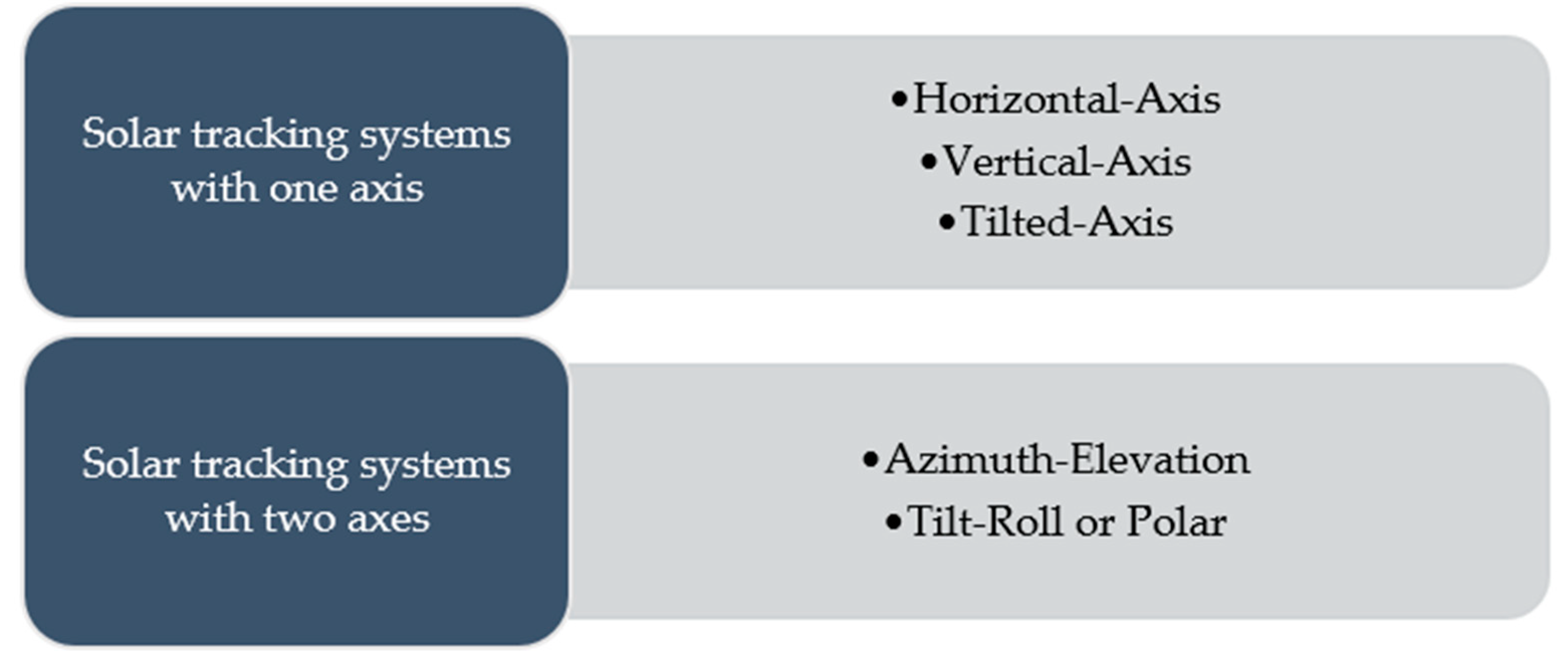
Figure 2.
Types of sun tracker solutions based on [
36].
Figure 2.
Types of sun tracker solutions based on [
36].
Figure 3.
The measuring station in Keszthely (1, HYTE-ANA-1735 humidity module [measuring air humidity]; 2, Pt 100 sensor; 3, manual/automatic tracking control unit; 4, m-Si module; 5, CPV module; 6, photosensors; 7, Eppley Black and White pyranometer; 8, a-Si module; 9, p-Si module; 10, Hukseflux LP02 pyranometers; 11, EMS 11 Silicon PV detector; 12, DS-2 Sonic anemometer; 13, OTT TRH relative humidity sensor; Orange dot: Pt 100 sensors).
Figure 4.
Fisheye view of the measuring station surroundings in the summer afternoon.
Figure 4.
Fisheye view of the measuring station surroundings in the summer afternoon.
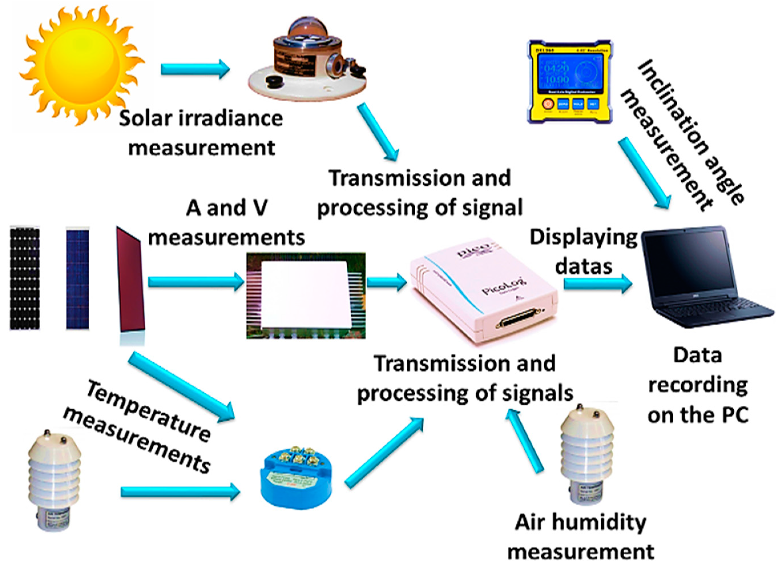
Figure 5.
Schematic illustration of PV module measuring station ‘A’.
Figure 5.
Schematic illustration of PV module measuring station ‘A’.
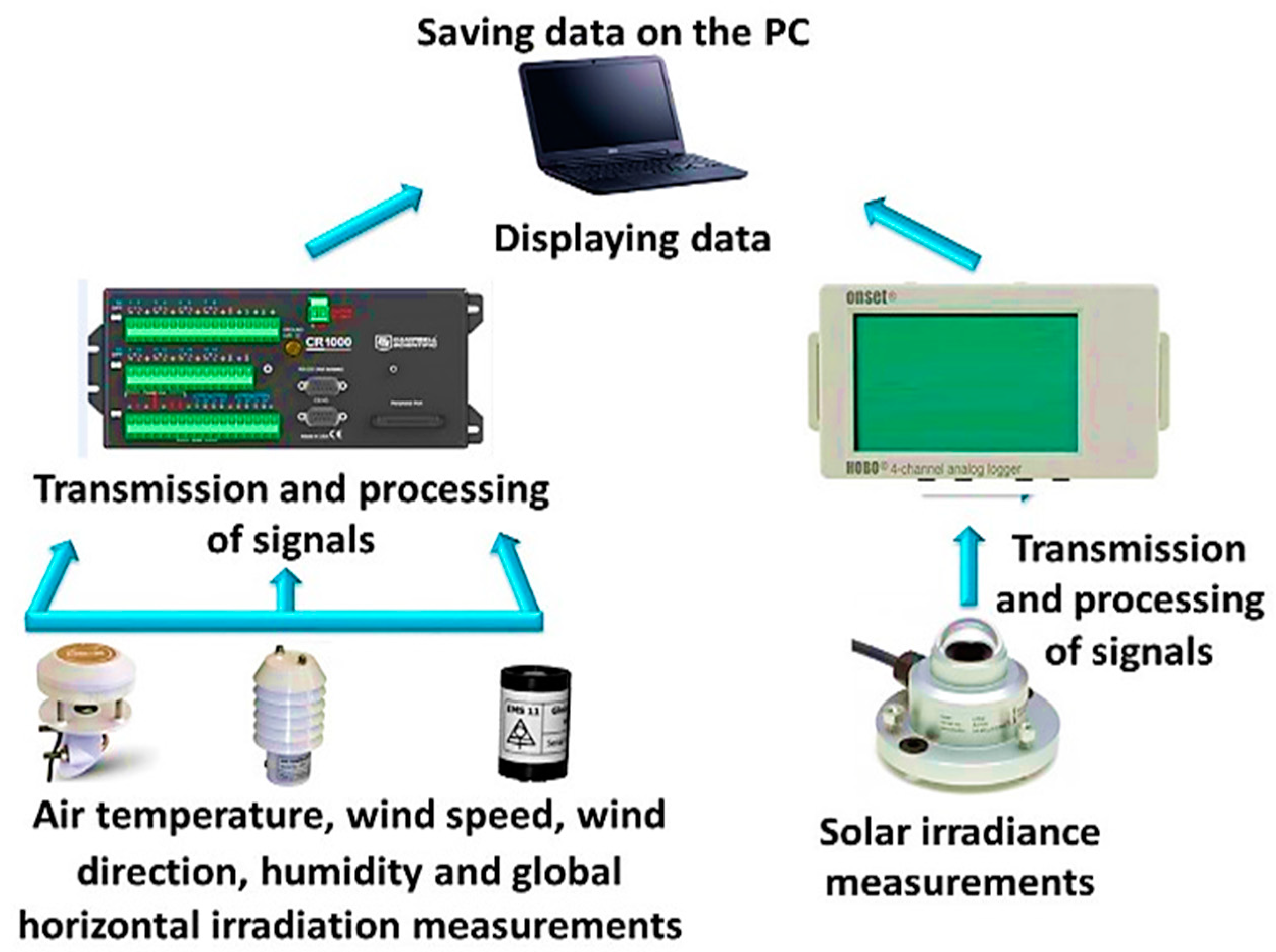
Figure 6.
Schematic illustration of PV module measuring station ‘B’.
Figure 6.
Schematic illustration of PV module measuring station ‘B’.
Figure 7.
The accuracy of the alignment to the sun can be illustrated with the help of the CPV cells (upper image: incorrect setting; lower image: precise setting).
Figure 7.
The accuracy of the alignment to the sun can be illustrated with the help of the CPV cells (upper image: incorrect setting; lower image: precise setting).
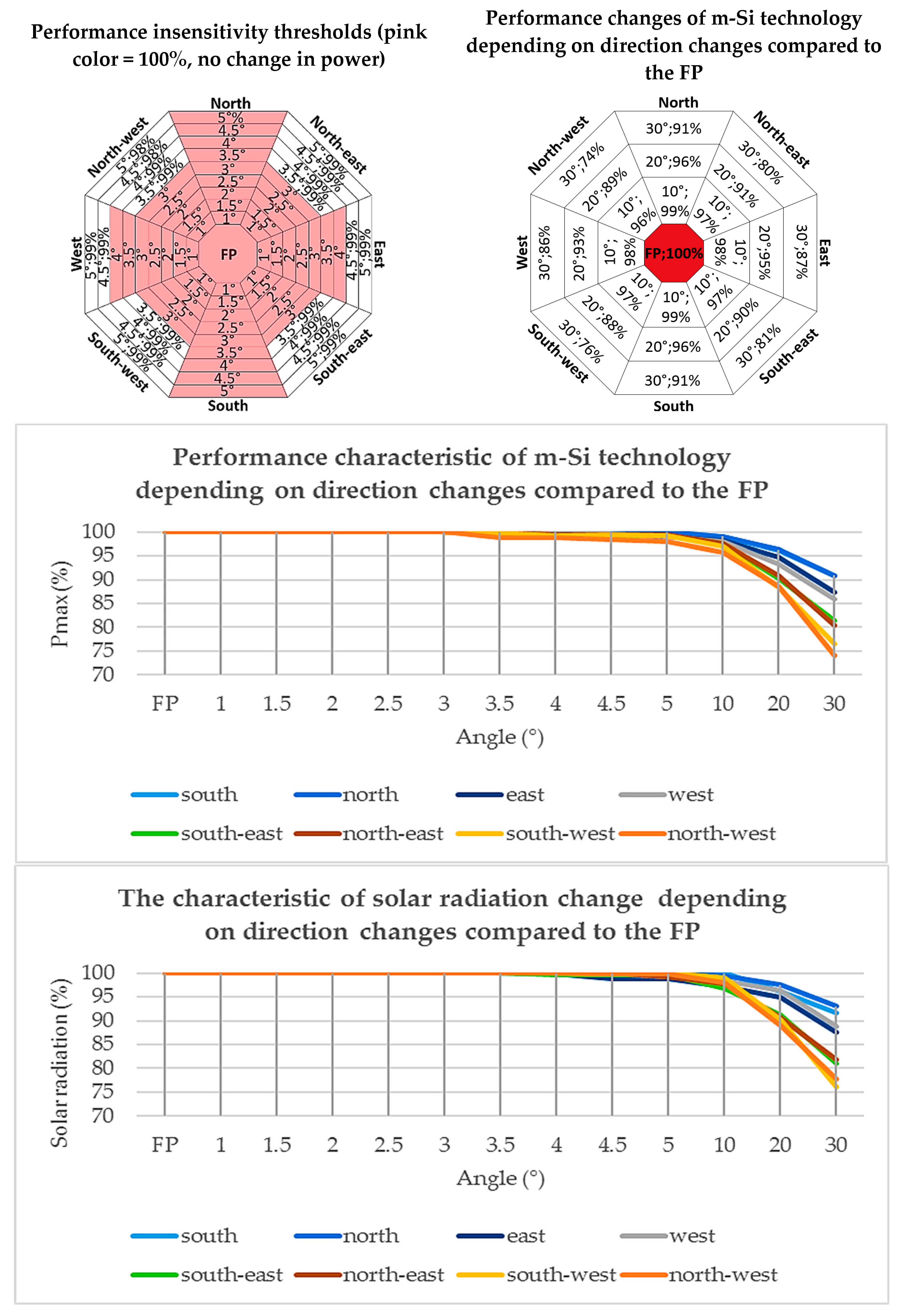
Figure 8.
The performance insensitivity thresholds, the performance changes, the solar radiation features and the performance characteristics of m-Si technology depending on directional changes compared to the focus point (FP).
Figure 8.
The performance insensitivity thresholds, the performance changes, the solar radiation features and the performance characteristics of m-Si technology depending on directional changes compared to the focus point (FP).
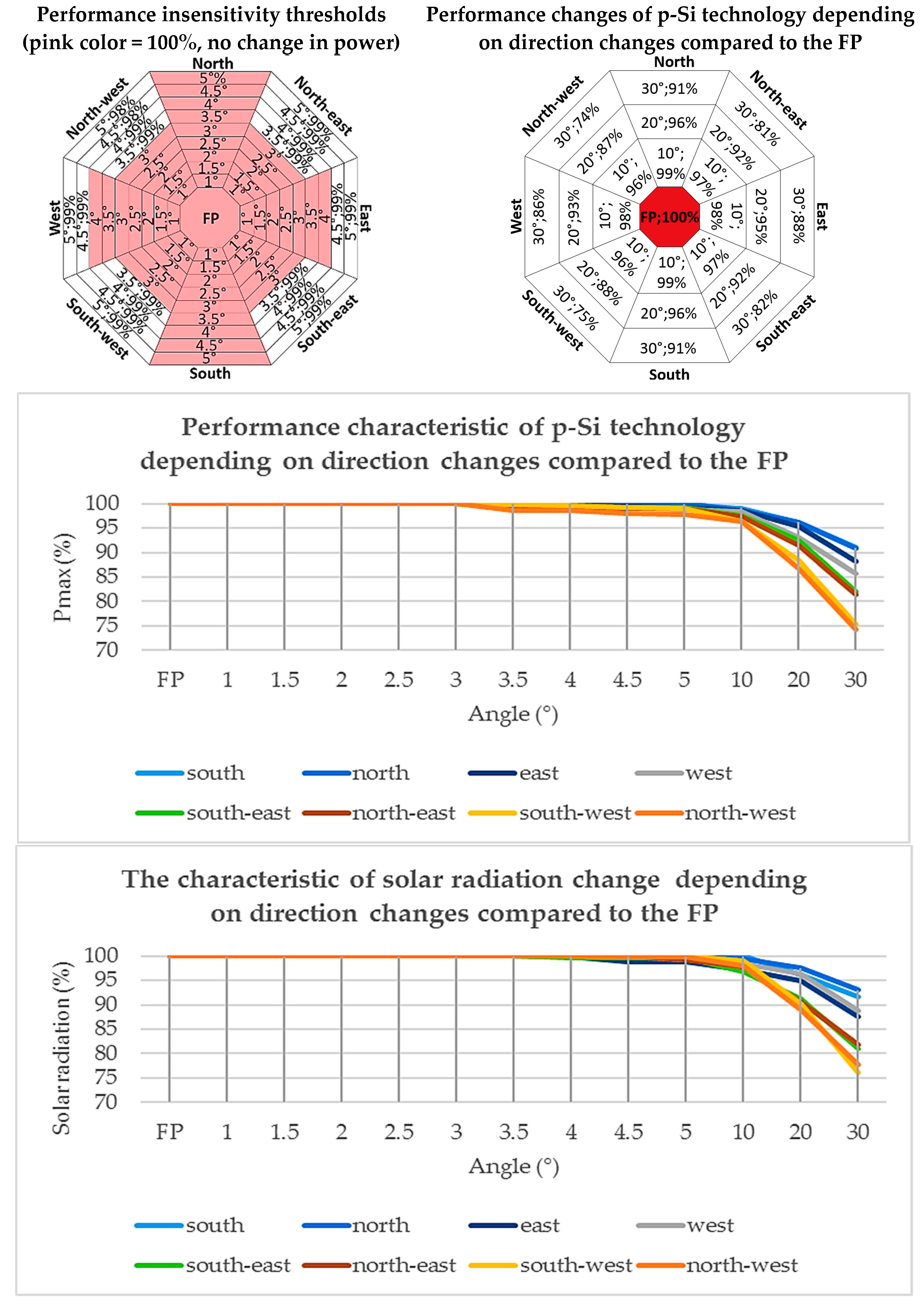
Figure 9.
The performance insensitivity thresholds, the performance changes, the solar radiation features and the performance characteristics of p-Si technology depending on directional changes compared to the FP.
Figure 9.
The performance insensitivity thresholds, the performance changes, the solar radiation features and the performance characteristics of p-Si technology depending on directional changes compared to the FP.
Figure 10.
The performance insensitivity thresholds, the performance changes, the solar radiation features and the performance characteristics of a-Si technology depending on directional changes compared to the FP.
Figure 10.
The performance insensitivity thresholds, the performance changes, the solar radiation features and the performance characteristics of a-Si technology depending on directional changes compared to the FP.
Table 1.
The gain in yearly real energy production compared to optimally positioned south-facing crystalline photovoltaic (PV) systems.
Table 1.
The gain in yearly real energy production compared to optimally positioned south-facing crystalline photovoltaic (PV) systems.
| Country (City/Town) | Gain in Yearly Real Energy Production Achieved by Using a Double-Axis Tracker System (%) | Reference |
|---|
| Turkey (Muğla) | 30.8 | [22] |
| Canada (Vermilion) | 31 | [49] |
| Spain (Palencia) | 30.5 | [50] |
| Greece (average) | 34.5 | [19] |
| Greece (Ilia) | 21 |
| Greece (Serres) | 27.4 |
| Greece (Karditsa) | 37.3 |
| Greece (Evros) | 42.2 |
| Greece (Kilkis) | 34.5 |
| Greece (Trikala) | 34.6 |
| Greece (Magnisia) | 39.1 |
| Greece (Rodopi) | 42.2 |
Table 2.
Technical information of the PV modules. (standard test conditions: air mass 1.5; cell temperature 25 °C; irradiance = 1000 W/m2/m-Si, p-Si, a-Si modules; irradiance = 850 W/m2/concentrator photovoltaic (CPV) module).
Table 2.
Technical information of the PV modules. (standard test conditions: air mass 1.5; cell temperature 25 °C; irradiance = 1000 W/m2/m-Si, p-Si, a-Si modules; irradiance = 850 W/m2/concentrator photovoltaic (CPV) module).
| Module Type | CPV | a-Si | m-Si | p-Si |
|---|
| Model | CX-75-III | G-EA050 | SM636-50 | SL50TU-18P |
|---|
| Nominal power (Pmax) (W) | 75 | 50 | 50 | 50 |
| Performance tolerance (%) | ±5% | ±10% | ±3% | ±3% |
| MPP voltage (Vmp) (V) | 135 | 67 | 18.18 | 19.12 |
| MPP current (Imp) (A) | 0.55 | 0.75 | 2.8 | 2.62 |
| Open circuit voltage (Voc) (V) | 150 | 91.8 | 23.17 | 22.68 |
| Short circuit current (Isc) (A) | 0.64 | 1.19 | 3.08 | 2.80 |
| Efficiency (%) | 27.2 | 5.3 | 14.4 | 13.7 |
| Temperature Coefficient (%/°C) | 0.15 | 0.27 | 0.5 | 0.5 |
Table 3.
The effect of solar radiation changes on m-Si performance. (x = change in solar radiation (%), FP = 100%, 80% = 20% change in solar radiation; f(x) = percentage value of the performance compared to the FP).
Table 3.
The effect of solar radiation changes on m-Si performance. (x = change in solar radiation (%), FP = 100%, 80% = 20% change in solar radiation; f(x) = percentage value of the performance compared to the FP).
| Description | Equation | Numerical Results for Modeling | R-Square |
|---|
| South | f(x) = p1 × x2 + p2 × x + p3 | p1 = −0.01395 | 0.9889 |
| p2 = 3.748 |
| p3 = −135.5 |
| North | p1 = 0.04104 | 0.9996 |
| p2 = −6.601 |
| p3 = 349.7 |
| East | p1 = −0.01577 | 0.9947 |
| p2 = 3.978 |
| p3 = −140.1 |
| West | p1 = 0.05651 | 0.9939 |
| p2 = −9.401 |
| p3 = 475.1 |
| South-east | p1 = 0.006652 | 0.9953 |
| p2 = −0.2319 |
| p3 = 56.61 |
| South-west | p1 = 0.01358 | 0.9943 |
| p2 = −1.421 |
| p3 = 105.9 |
| North-east | p1 = −0.01195 | 0.9987 |
| p2 = 3.244 |
| p3 = −105 |
| North-west | p1 = −0.009231 | 0.9880 |
| p2 = 2.776 |
| p3 = −85.95 |
| Example of calculation result, south-east, 80% change in solar radiation [%] | 81% = p1 × 802 + p2 × 80 + p3 | |
Table 4.
The effect of solar radiation changes on p-Si performance (x = change in solar radiation (%), FP = 100%, 80% = 20% change in solar radiation; f(x) = percentage value of the performance compared to the FP).
Table 4.
The effect of solar radiation changes on p-Si performance (x = change in solar radiation (%), FP = 100%, 80% = 20% change in solar radiation; f(x) = percentage value of the performance compared to the FP).
| Description | Equation | Numerical Results for Modeling | R-Square |
|---|
| South | f(x) = p1 × x2 + p2 × x + p3 | p1 = −0.01918 | 0.9910 |
| p2 = 4.745 |
| p3 = −182.8 |
| North | p1 = 0.06783 | 0.9963 |
| p2 = −11.8 |
| p3 = 601.7 |
| East | p1 = −0.02172 | 0.9926 |
| p2 = 5.032 |
| p3 = −185.9 |
| West | p1 = 0.05355 | 0.9827 |
| p2 = −8.834 |
| p3 = 447.7 |
| South-east | p1 = −0.009841 | 0.9985 |
| p2 = 2.717 |
| p3 = −73.46 |
| South-west | p1 = 0.01107 | 0.9910 |
| p2 = −0.9367 |
| p3 = 82.5 |
| North-east | p1 = −0.01228 | 0.9957 |
| p2 = 3.236 |
| p3 = −101.1 |
| North-west | p1 = 0.002913 | 0.9898 |
| p2 = 0.6102 |
| p3 = 9.131 |
| Example of calculation result, south-east, 20% change in solar radiation [%] | 81% = p1 × 802 + p2 × 80 + p3 | |
Table 5.
The effect of solar radiation changes on a-Si performance (x = change in solar radiation (%), FP = 100%, 80% = 20% change in solar radiation; f(x) = percentage value of the performance compared to the FP).
Table 5.
The effect of solar radiation changes on a-Si performance (x = change in solar radiation (%), FP = 100%, 80% = 20% change in solar radiation; f(x) = percentage value of the performance compared to the FP).
| Description | Equation | Numerical Results for Modeling | R-Square |
|---|
| South | f(x) = p1 × x2 + p2 × x + p3 | p1 = −0.01557 | 0.9933 |
| p2 = 4.28 |
| p3 = −172.4 |
| North | p1 = 0.0601 | 1 |
| p2 = −10 |
| p3 = 499.2 |
| East | p1 = −0.01756 | 0.9948 |
| p2 = 4.468 |
| p3 = −171.3 |
| West | p1 = 0.06519 | 0.9929 |
| p2 = −10.82 |
| p3 = 530.1 |
| South-east | p1 = 0.01088 | 0.9942 |
| p2 = −0.7589 |
| p3 = 67.21 |
| South-west | p1 = 0.01088 | 0.9956 |
| p2 = −0.6964 |
| p3 = 60.43 |
| North-east | p1 = −0.01392 | 0.9990 |
| p2 = 3.776 |
| p3 = −138.5 |
| North-west | p1 = 0.004485 | 0.9957 |
| p2 = 0.5934 |
| p3 = −4.726 |
| Example of calculation result, south-east, 20% change in solar radiation [%] | 76% = p1 × 802 + p2 × 80 + p3 | - |
Table 6.
The effect of directional changes on m-Si performance (x = change in orientation (°); f(x) = percentage value of the performance compared to the FP).
Table 6.
The effect of directional changes on m-Si performance (x = change in orientation (°); f(x) = percentage value of the performance compared to the FP).
| Description | Equation | Numerical Results for Modeling | R-Square |
|---|
| South | f(x) = p1 × x4 + p2 × x3 + p3 × x2 + p4 × x + p5 | p1 = −1.683 × 10⁻⁵ | 0.9998 |
| p2 = 0.0009611 |
| p3 = −0.02697 |
| p4 = 0.09686 |
| p5 = 99.95 |
| North | p1 = −1.877 × 10⁻⁵ |
| p2 = 0.0009883 |
| p3 = −0.02603 |
| p4 = 0.09122 |
| p5 = 99.95 |
| East | p1 = −4.017 × 10⁻⁵ | 0.9979 |
| p2 = 0.001883 |
| p3 = −0.03404 |
| p4 = −0.01403 |
| p5 = 100.1 |
| West | p1 = −2.936 × 10⁻⁵ | 0.9987 |
| p2 = 0.001704 |
| p3 = −0.04316 |
| p4 = 0.08324 |
| p5 = 100 |
| South-east | p1 = 2.095 × 10⁻⁵ | 0.9994 |
| p2 = −0.0007642 |
| p3 = −0.01447 |
| p4 = −0.06451 |
| p5 = 100.1 |
| South-west | p1 = −3.515 × 10⁻⁶ | 0.9996 |
| p2 = 0.0004726 |
| p3 = −0.03775 |
| p4 = 0.01547 |
| p5 = 100.1 |
| North-east | p1 = −8.536 × 10⁻⁶ | 0.9997 |
| p2 = 0.0006003 |
| p3 = −0.03319 |
| p4 = 0.03196 |
| p5 = 100 |
| North-west | p1 = −6.333 × 10⁻⁵ | 0.9987 |
| p2 = 0.002912 |
| p3 = −0.05449 |
| p4 = −0.1513 |
| p5 = 100.3 |
| Example of calculation result, south-east, 20% direction change [%] | 90% = p1 × 204 + p2 × 203 + p3 × 202 + p4 × 20 + p5 | |
Table 7.
The effect of directional changes on p-Si performance (x = change in orientation (°); f(x) = percentage value of the performance compared to the FP).
Table 7.
The effect of directional changes on p-Si performance (x = change in orientation (°); f(x) = percentage value of the performance compared to the FP).
| Description | Equation | Numerical Results for Modeling | R-Square |
|---|
| South | f(x) = p1 × x4 + p2 × x3 + p3 × x2 + p4 × x + p5 | p1 = −1.17 × 10⁻⁵ | 0.9999 |
| p2 = 0.0006521 |
| p3 = −0.02167 |
| p4 = 0.07924 |
| p5 = 99.96 |
| North | f(x) = p1 × x3 + p2 × x2 + p3 × x + p4 | p1 = −2.369 × 10⁻⁵ | 0.9956 |
| p2 = −0.008792 |
| p3 = −0.02042 |
| p4 = 100.1 |
| East | f(x) = p1 × x4 + p2 × x3 + p3 × x2 + p4 × x + p5 | p1 = −1.88 × 10⁻⁵ | 0.9981 |
| p2 = 0.0007663 |
| p3 = −0.01851 |
| p4 = −0.0239 |
| p5 = 100.1 |
| West | f(x) = p1 × x3 + p2 × x2 + p3 × x + p4 | p1 = −6.694 × 10⁻⁵ | 0.9935 |
| p2 = −0.01025 |
| p3 = −0.1163 |
| p4 = 100.1 |
| South-east | f(x) = p1 × x4 + p2 × x3 + p3 × x2 + p4 × x + p5 | p1 = −3.306 × 10⁻⁵ | 0.9996 |
| p2 = 0.001555 |
| p3 = −0.03691 |
| p4 = −0.002006 |
| p5 = 100.1 |
| South-west | p1 = −2.717 × 10⁻⁵ | 0.9985 |
| p2 = 0.001542 |
| p3 = −0.04935 |
| p4 = 0.001848 |
| p5 = 100.1 |
| North-east | p1 = −2.624 × 10⁻⁵ | 0.9993 |
| p2 = 0.001321 |
| p3 = −0.0354 |
| p4 = −0.03995 |
| p5 = 100.1 |
| North-west | f(x) = p1 × x3 + p2 × x2 + p3 × x + p4 | p1 = −2.968 × 10⁻⁵ | 0.9961 |
| p2 = −0.01921 |
| p3 = −0.2668 |
| p4 = 100.2 |
| Example of calculation result, south-east, 20% direction change [%] | 92% = p1 × 204 + p2 × 203 + p3 × 202 + p4 × 20 + p5 | |
Table 8.
The effect of directional changes on a-Si performance (x = change in orientation (°); f(x) = percentage value of the performance compared to the FP).
Table 8.
The effect of directional changes on a-Si performance (x = change in orientation (°); f(x) = percentage value of the performance compared to the FP).
| Description | Equation | Numerical Results for Modeling | R-Square |
|---|
| South | f(x) = p1 × x4 + p2 × x3 + p3 × x2 + p4 × x + p5 | p1 = 2.646 × 10⁻⁷ | 0.9999 |
| p2 = 5.382 × 10⁻⁵ |
| p3 = −0.01624 |
| p4 = 0.06834 |
| p5 = 99.96 |
| North | f(x) = p1 × x3 + p2 × x2 + p3 × x + p4 | p1 = 3.102 × 10⁻⁵ | 0.9998 |
| p2 = −0.01546 |
| p3 = 0.06449 |
| p4 = 99.97 |
| East | f(x) = p1 × x4 + p2 × x3 + p3 × x2 + p4 × x + p5 | p1 = −4.779 × 10⁻⁵ | 0.9984 |
| p2 = 0.002246 |
| p3 = −0.04004 |
| p4 = −0.02006 |
| p5 = 100.1 |
| West | p1 = −3.919 × 10⁻⁵ | 0.9994 |
| p2 = 0.002307 |
| p3 = −0.05705 |
| p4 = 0.1432 |
| p5 = 99.97 |
| South-east | p1 = 3.445 × 10⁻⁵ | 0.9999 |
| p2 = −0.001102 |
| p3 = −0.02458 |
| p4 = 0.03649 |
| p5 = 100 |
| South-west | p1 = −1.174 × 10⁻⁶ | 0.9996 |
| p2 = 0.0002058 |
| p3 = −0.03832 |
| p4 = 0.01014 |
| p5 = 100.1 |
| North-east | p1 = 7.699 × 10⁻⁶ | 0.9998 |
| p2 = −0.0002437 |
| p3 = −0.02453 |
| p4 = −0.01247 |
| p5 = 100.1 |
| North-west | p1 = 7.456 × 10⁻⁵ | 0.9984 |
| p2 = −0.003751 |
| p3 = 0.02249 |
| p4 = −0.373 |
| p5 = 100.4 |
| Example of calculation result, south-east, 20% direction change [%] | 88% = p1 × 204 + p2 × 203 + p3 × 202 + p4 × 20 + p5 | |

 ,
, 


