The Hay Inclined Plane in Coalbrookdale (Shropshire, England): Analysis through Computer-Aided Engineering

Abstract

This article analyzes the ‘Hay inclined plane’ designed by the English engineer and entrepreneur William Reynolds and put into operation in 1792 to facilitate the transport of vessels between channels at different levels using an inclined plane. To this end, a study of computer-aided engineering (CAE) was carried out using the parametric software Autodesk Inventor Professional, consisting of a static analysis using the finite-element method (FEM) of the 3D model of the invention under real operating conditions. The results obtained after subjecting the mechanism to the two most unfavorable situations (blockage situation of the inertia flywheel and emergency braking situation) indicate that, with the exception of the braking bar, the rest of the assembly is perfectly designed and dimensioned. In particular, for the blockage situation, the point with the greatest stress is at the junction between the inertia flywheel and the axle to which it is attached, the maximum value of von Mises stress being at that point (186.9 MPa) lower than the elastic limit of the cast iron. Also, at this point the deformation is very low (0.13% of its length), as well as the maximum displacement that takes place in the inertia flywheel itself (22.98 mm), and the lowest safety factor has a value of 3.51 (located on the wooden shaft support), which indicates that the mechanism is clearly oversized. On the other hand, the emergency braking situation, which is technically impossible with a manual operation, indicates that the braking bar supports a maximum von Mises stress of 1025 MPa, above the elastic limit of the material, so it would break. However, other than that element, the rest of the elements have lower stresses, with a maximum value of 390.7 MPa, and with safety factors higher than 1.7, which indicates that the mechanism was well dimensioned.

1. Introduction

The work presented in this article was developed within a research project on the work of Agustín de Betancourt [1,2,3], analyzing his best-known inventions both from the point of view of engineering graphics [4,5,6,7] and from the point of view of mechanical engineering [8,9,10,11,12].

The article shows the static analysis carried out on the inclined plane for the transport of vessels that operated in Coalbrookdale (Shropshire, England) at the end of the 18th century. This historical invention, popularly known as ‘The Hay inclined plane’, and the work of the Englishman William Reynolds, made possible the transportation of boats between channels located at different levels.

This invention was the object of a very detailed study from the point of view of engineering graphics [13] that allowed us to obtain a reliable 3D model, from which the research presented in this article was carried out. There is no study from the point of view of mechanical engineering worldwide of this historical invention, a fact which underlines its novelty and scientific interest. The invention had a remarkable influence on the socioeconomic development of the region, as it was of considerable benefit for the coal mines and blacksmiths of the zone, since it allowed the commerce of their products through the river Severn, and the fluvial port Coalport on this river grew to be an important industrial hub [14].

The Shropshire canal was created in 1790 and closed to river traffic in 1944. This bi-directional inclined plane, which had a length of 350 yards (320 m) and allowed vessels to ascend and descend, was put into operation in 1792, and negotiated a difference of 210 feet (64 m).

Meanwhile, Agustín de Betancourt had dedicated much of his research to the study of navigation channels [1], and during his stay in England (1793–1796) he copied in detail the mechanism as it was built, drawing a color sheet of the inclined plane with much detail and a three-page handwritten account explaining the parts of the plane and its operation. These are the only documents of which there is evidence in reference to the inclined plane of Coalbrookdale [15]. The advantage of this historical invention was that it allowed a large drop to be negotiated without loss of water in the process of the ascent and descent of the boats.

Later, Agustín de Betancourt published his work ‘Mémoire sur un nouveau système de navigation intérieure’ written in Paris in 1807 [16], in which he proposes a channel navigation system for France very similar to the English navigation system: shallow channels and with an advanced system of locks that avoid loss of water in the ascent and descent of the boats. In this account, Betancourt applies his plunger lock to the inclined plane, and mentions the previous work of Robert Fulton [17], indicating that his inclined plane is designed according to Reynolds’ procedure.

At present, only ruins remain of the inclined plane of Coalbrookdale. Some photographs [18] still show the inclined plane and the remains of the rails, although it is also possible to distinguish the upper cargo basin and the remains of the brick building that housed the steam engine.

The ultimate goal of this research is to perform a static analysis [19] of the Hay inclined plane using the finite element method (FEM) [20] under real operating conditions, in order to determine whether it was well dimensioned and functioned properly. Its scientific interest lies in the fact that from the point of view of industrial archaeology and the study of technical historical heritage, there is no existing study, worldwide, on this outstanding example of industrial historical heritage, which marked a historic milestone in the Industrial Revolution (1760–1840). This underscores the utility and originality of this research.

The remainder of the paper is structured as follows: Section 2 presents the materials and methods used in this investigation; then, Section 3 includes the main results such as von Mises stresses, displacements, deformations and safety coefficient; and Section 4 shows the main conclusions.

2. Materials and Methods

As mentioned above, the article has as its starting point the 3D model of the Hay inclined plane developed through our own methodology and published in a previous article [13]. Static analysis of this 3D model by means of FEM has been proposed.

Therefore, the sources used for the present study are the same as those used to obtain the 3D model. The Orotava Canary Foundation for the History of Science [21] developed a project on the engineer Agustín de Betancourt in which all his written and graphic work has been digitized [22]. In the file of the Spanish engineer [15], there is a written account and a detailed sheet of the existing inclined plane in Coalbrookdale that operated between the River Severn and the Shropshire Canal. The colored sheet, drawn by hand by Betancourt himself, describes most of the elements of William Reynolds’ ingenuity, but cannot be considered as a scale plane itself, since without a written account it is impossible to understand the functioning of the mechanism for moving ascending and descending boats and, in addition, because some of the parts of the mechanism do not appear to be detailed in the plan, although they do in the written account.

2.1. Operation of the Hay Inclined Plane

To give the reader a complete idea of the analysis of the invention of William Reynolds, it is necessary to explain its operation. An exhaustive description of the mechanism is included in the article published on obtaining the 3D model [13], so a more summarized description will be given here.

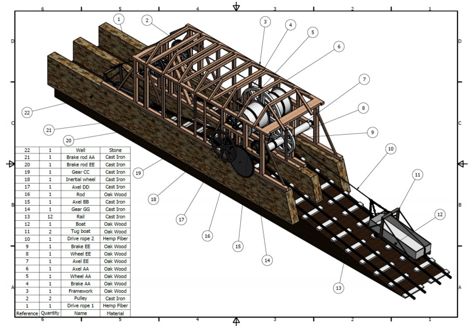
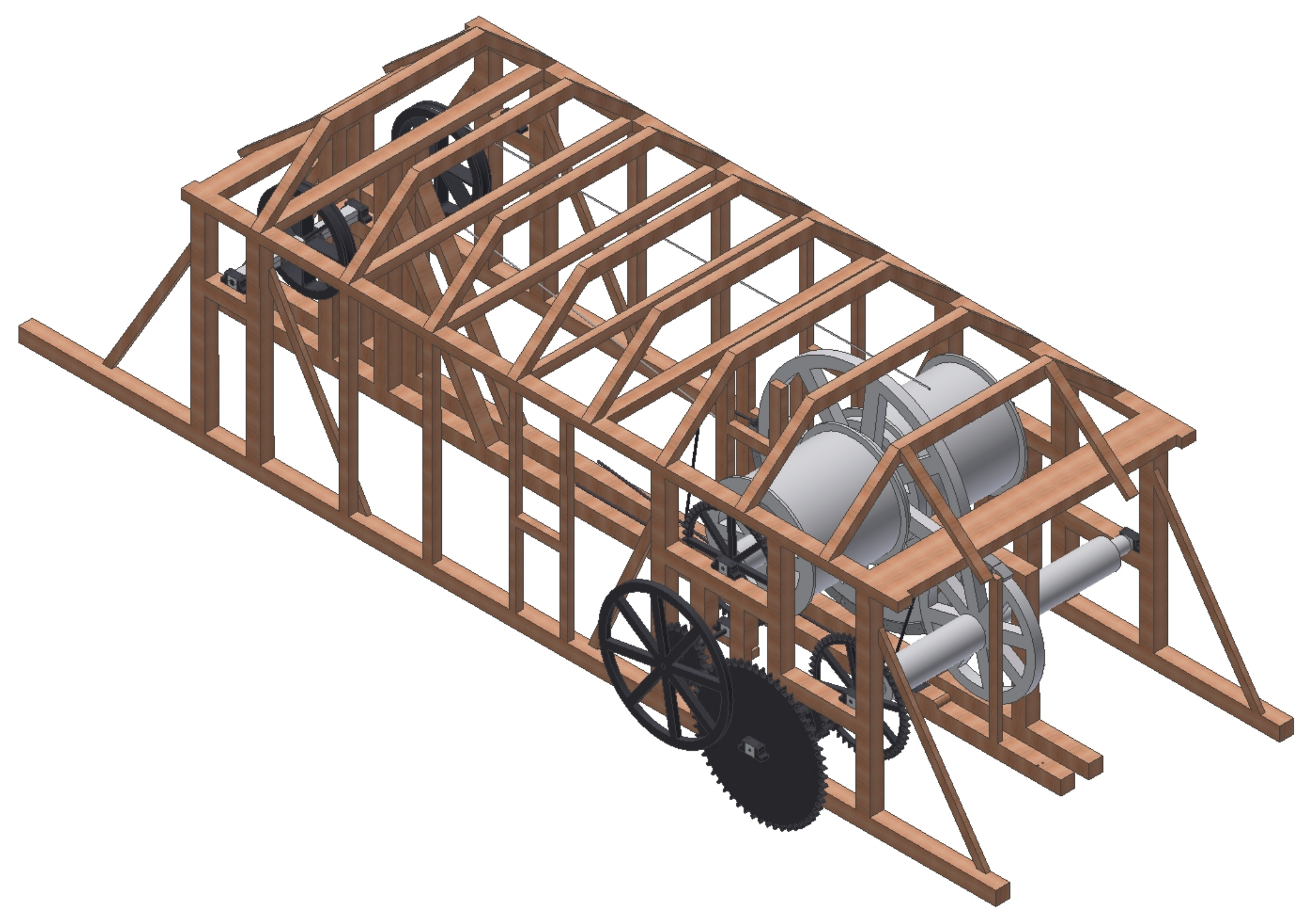
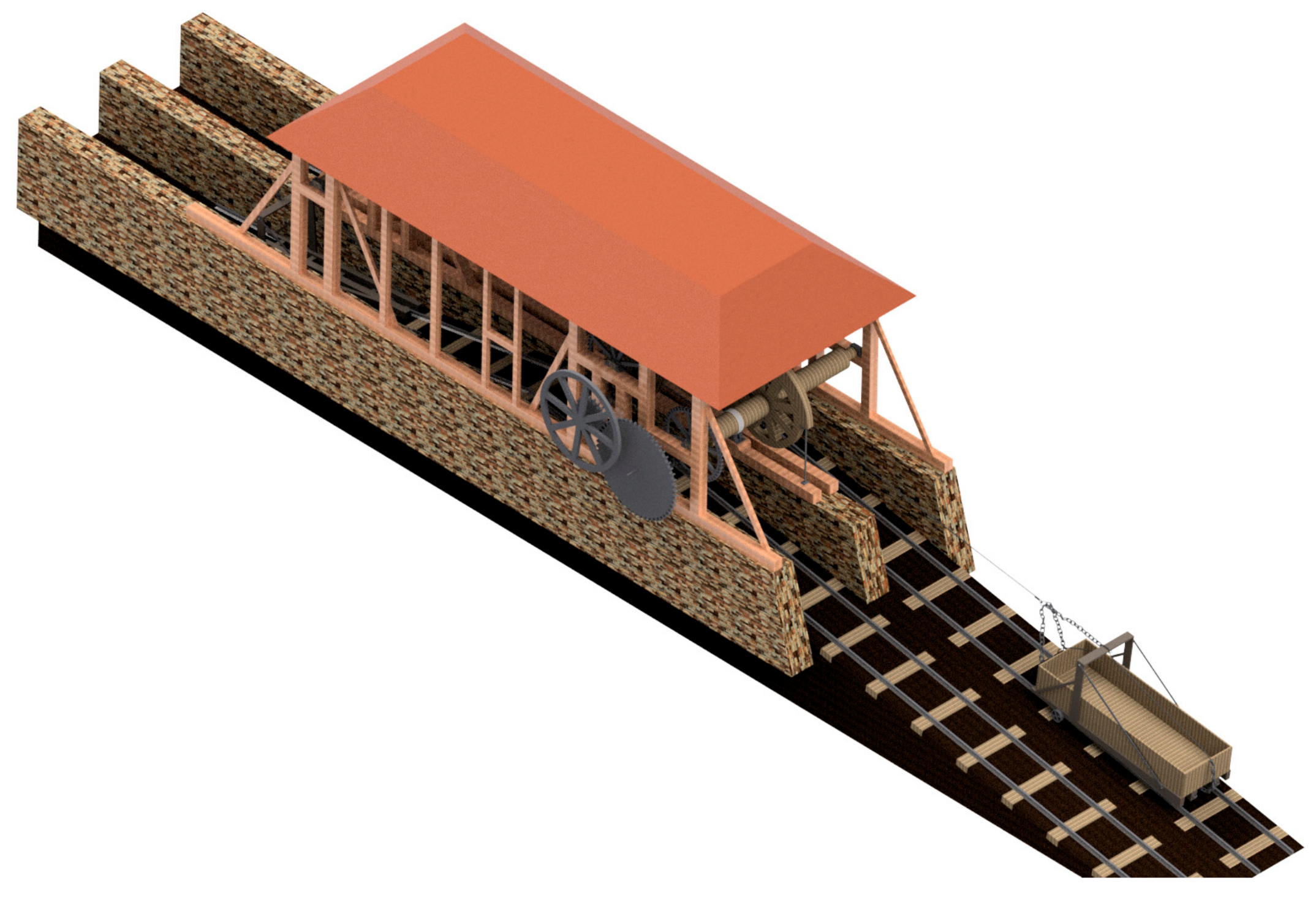
Figure 1 shows an isometric view of the mechanism after its computer-aided design (CAD) modeling, and Figure 2 shows a plan of the ensemble with an indicative list of the different elements that form it. Figure 2, Figure 3 and Figure 4 will serve to illustrate the operation of the mechanism.

2.1.1. Upward Movement

For the ascent of the boats (12), the tugboat (11) waited in the lower partially submerged part. The boat loaded with the material to be transported was placed on the tugboat, and they were tied together with a chain. After sending a signal to the operator of the upper station, a rope pulled the trailer, helping it to ascend on the rails (13).

The rope (10) that pulled the boat was picked up in the upper station on the AA axle drum (6) after going through some pulleys (2). As the axle rotated, the rope was coiled and the boat ascended. To move this axle, a steam engine was necessary, which moved a series of gears. An adjacent steam engine, of which only the chimney and the brick building where it was housed remain, operated an inertia flywheel (18). The wheel was solidly attached to the DD axle (17), which had two gears. The distal gear, which was the smaller gear, was coupled to the CC gear (19), which was the larger gear, which was solidly attached to axle AA, so that for each turn of the inertia flywheel the AA axle rotated 0.098 times in the opposite direction.

At the same time, the DD axle had a gear close to the inertia flywheel larger than the distal one. This gear meshed with an intermediate shaft, axle BB (15), which finally transmitted the movement to axle EE (7). For each turn that the inertia flywheel gave, the EE axle rotated, in the same direction, 0.14 times. A second rope pulling the tugboat that was in the upper channel was wound onto the EE axle drum.

To prevent the load from falling, or when it was necessary to move more slowly, two brakes could be used that braked the AA axle (4) or the EE axle (9) independently. For this, each axle had an inertia flywheel on which the brake was held, so that when pulling one of the braking levers (20) and (21), a collar embraced the wheels (8) and (5), respectively, and reduced the speed of the axles by friction.

2.1.2. Downward Movement

To descend the boats through the inclined plane, the process was similar. The path that had served to ascend the boat was automatically transformed into a descent route and vice versa. The engine had two hemispheres, where the ropes were wound onto the axles in the opposite direction, so while one of the axles was rolled, the other was unrolled with the same movement. When the rope was fully wound onto the drum, the end was taken on the other side of the drum, passed back through the pulley, and began to unroll.

The boat towed in the upper channel was pulled by the rope (1) attached to the EE axle to the upper station. In the upper station of the inclined plane, the rope was changed, and it was joined to the AA axle rope (10), which slowly began to unwind, allowing the plane to descend in a controlled manner. In cases of urgent necessity, both in the ascending and descending movement, the axle of the inertia flywheel DD (17) could be disconnected from the rest of the gears by actuating the shaft support bar (16).

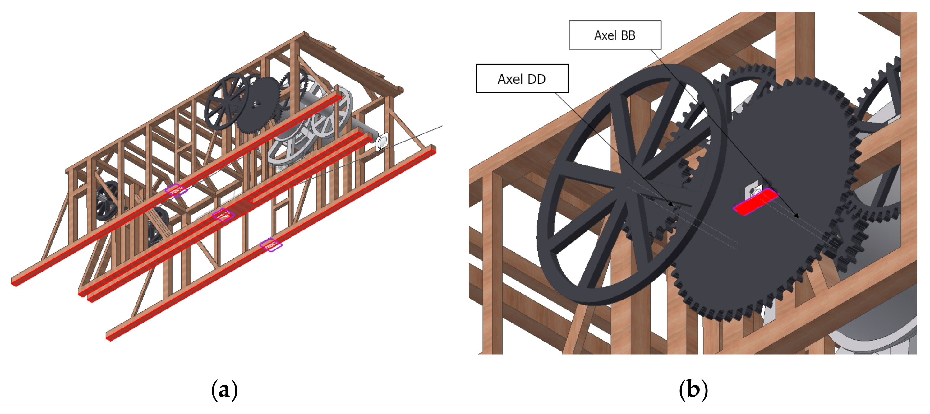
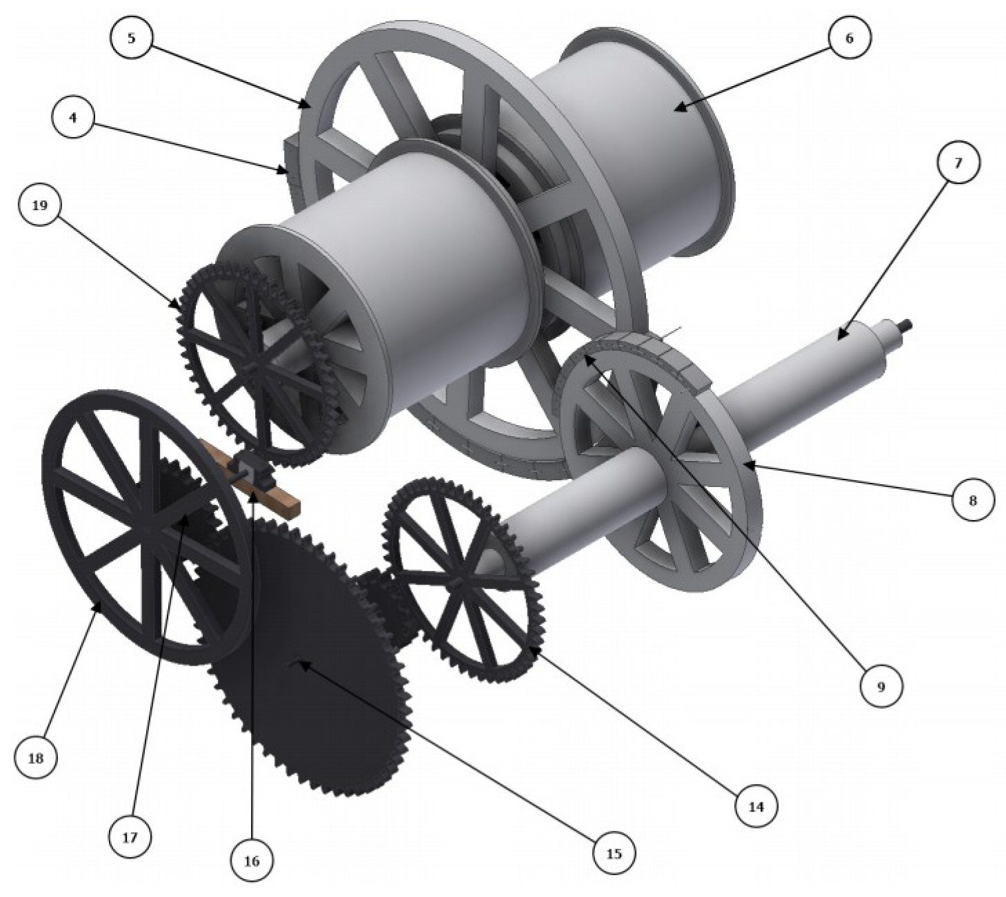
Figure 3 shows the detail of the axles and gears that facilitated the movement of the ropes. It is interesting to note that each of the axles has an inertia flywheel on which is placed a friction collar that functions as a brake. It is also possible to appreciate the moving bar of the DD axle support that serves to leave the entire set of transmissions motionless if necessary.

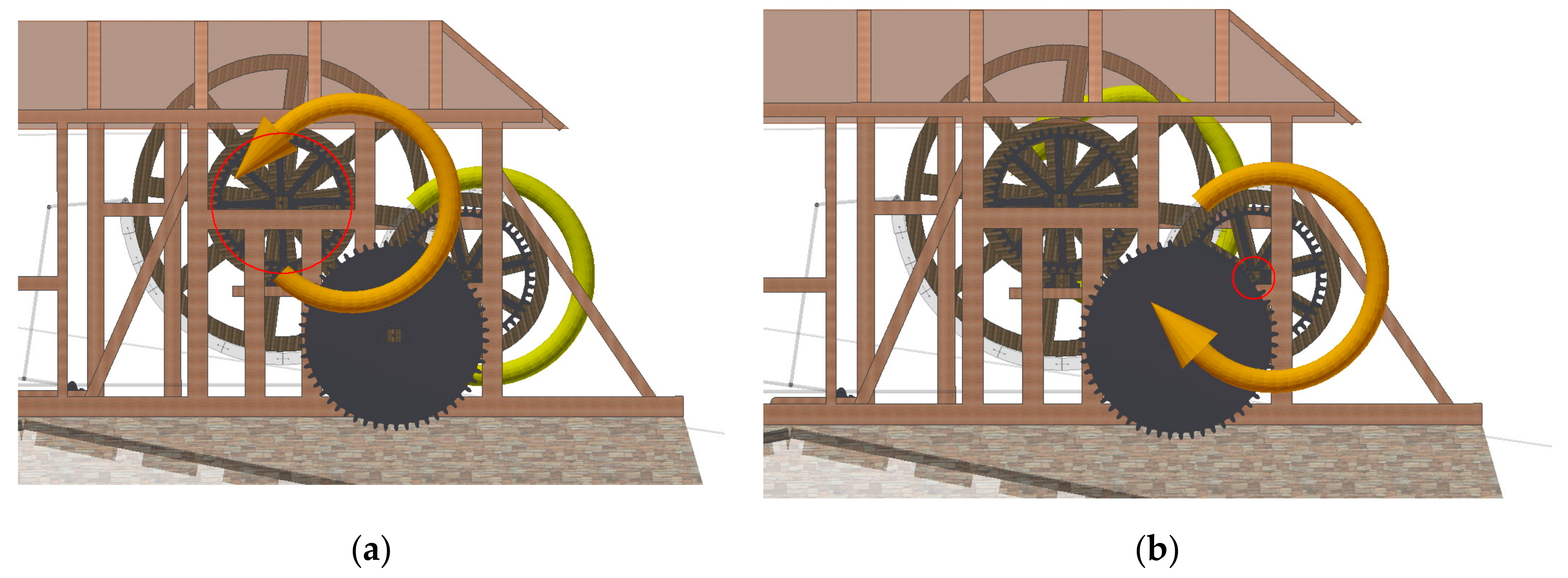
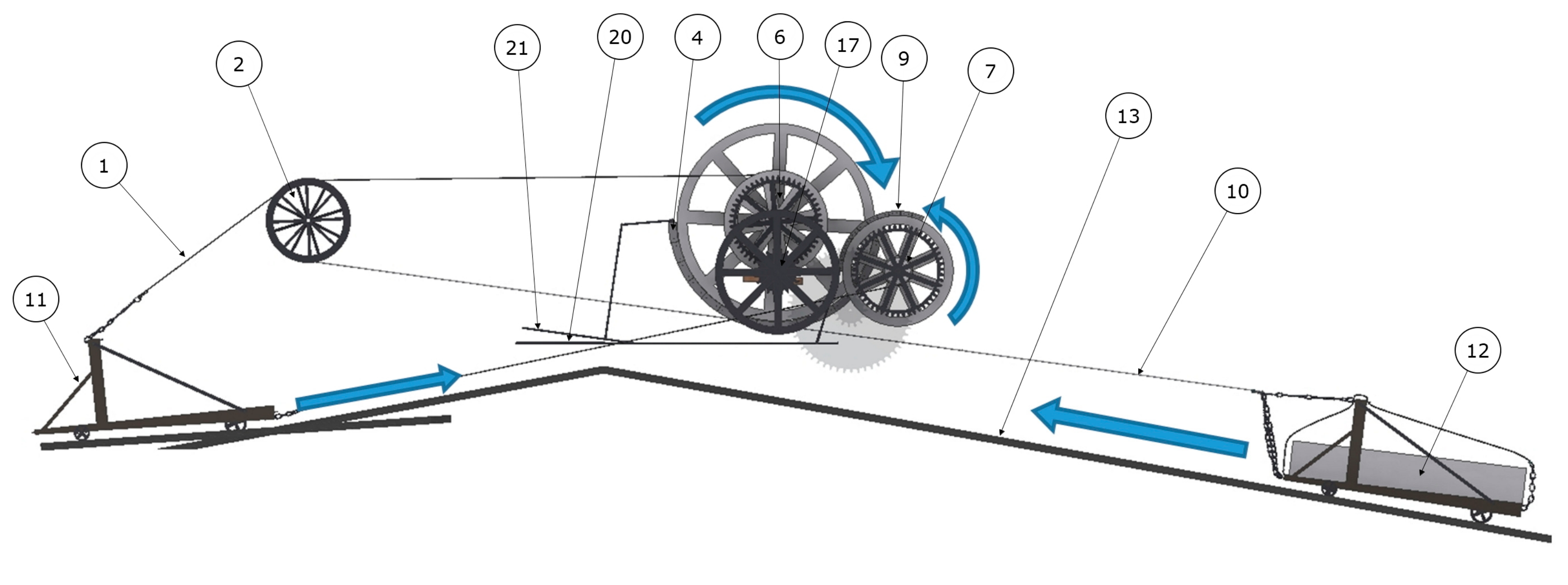
Figure 4 helps describe the movement of axles and tugboats when they are in upward motion. In the case indicated, the tugboat on the right is ascending to the upper channel and the one on the left, at that moment empty, is directed to the lower channel.

2.2. Computer-Aided Engineering (CAE)

Having defined and modeled the invention as designed by William Reynolds, it is now time to perform the static analysis with FEM, using Autodesk Inventor Professional software [23]. FEM is a numerical method used to solve differential equations by converting them into a linear system of equations. The results obtained by this method are only approximate, since a specific number of solutions are obtained for some points called “nodes”, while in the rest of the points, the solution is interpolated, obtaining an approximate value. Likewise, the processes and parameters in a finite-element analysis (FEA) are independent of the software used.

This method pursues two objectives: the modal analysis that evaluates the natural frequency modes, including the movements of rigid bodies, and the static analysis of the invention, which evaluates its load conditions.

The numerical method used for static analysis generates a matrix with a large number of parameters, which can be categorized into three types: movement restrictions of the elements, the physical characteristics of the materials used, and the loads that affect it. On the other hand, the numerical model of the modal analysis is generated with fewer parameters, depending only on the restrictions and the physical characteristics of the elements, and therefore it is not conditioned by the parameters related to the loads.

Based on these data, the static analysis will obtain results on the von Mises stresses, and the equivalent deformations and displacements of all the elements of the model, while the eight lowest natural frequencies in which the elements of the model enter into resonance will be determined in the modal analysis.

Then the set of parameters that determine the analysis will be the simplification and definition of the model (pre-processing), assignment of materials, definition of boundary conditions and study of loads.

On the other hand, the “nodes” are not determined randomly. To obtain a result that represents the whole mechanism, a network of nodes called a “mesh” is established, which must be adapted to the geometry of each element that takes a similar form. This process is called “discretization”, and each space delimited by the network is a “finite element”. These elements have different shapes (surfaces, volumes or bars). To complete the analysis, it will be necessary to define the shape of the mesh (geometry and size), since the number of nodes depends, to a large extent, on the accuracy of the FEM. The more nodes the model has, the higher will be the precision, but also the calculation matrix and, therefore, the calculation time needed by the processor.

2.2.1. Pre-Processing

The first step before proceeding with the simulation of the static analysis is the pre-processing. The invention for ascending and descending boats presents a high number of elements, meaning that excessive computational time would be required to perform the calculations required by FEM. As will be indicated below, the software used estimates more than one million elements that must be analyzed, which would require a great deal of time on a personal computer with standard features.

Therefore, a simplification of the model is necessary (Figure 5) to facilitate the simulation. However, the simplification of the model should be performed with caution, as it should not interfere with the results of the static analysis. In addition, we must bear in mind that it is impossible to study the invention working in all possible circumstances, since these can all be very different. Taking these two premises into account, the static analysis of the inclined plane will be carried out in the two most unfavorable situations.

In the first place, the brick building, the rails and the plan have been dispensed with, focusing the study on seeing how both the engine and the support structure are affected. The roof, being a light structure exposed to the weather, has also been eliminated from the simulation, since it is not the support structure of the plane and it is not the object of the present study to analyze how it behaves in relation to the different types of external load (snow or wind).

Furthermore, it has also been decided to dispense with boats and tugboats. Each one of them presents a very high number of elements that would considerably multiply the calculations without affecting the results. Therefore, each of the tugboats has been replaced with a force that will later become the object of study.

The ropes that are associated with the two traction axles have also been dispensed with. The ropes of the time, made of hemp, are elements that had a special behavior. The software used is not prepared to correctly characterize its dynamic properties, which would force us to replace the tensions of the ropes with forces in the pulleys or by torques in the shafts.

Finally, it is necessary to examine the situations in which the engine is to be studied. On the one hand, the study of the invention was carried out with the boats fully loaded and ascending to the upper station. A priori, this case produces the maximum stress on all gears, pulleys and axles, so it is really convenient to study. However, the brakes, which are also important elements of the invention, would not come into play in this situation, so it was determined to study a second situation.

Therefore, a first situation would be to analyze the invention in the case of a blockage of the inertia flywheel, due to a disconnection with the steam engine, when the boat is fully loaded and descending. Another case, which would correspond to a second situation of emergency braking, would be the case of the tugboat with a loaded boat that had to be stopped using the brake that embraces the inertia flywheel of the AA axle.

2.2.2. Assignment of Materials

Having understood what aspects of the invention are to be studied, it is necessary to verify that all the elements of the assembly have their physical characteristics perfectly defined, without which the static analysis cannot be performed. However, the original materials of the engine are specified neither in the description of the invention nor in the written account, but it is not excessively complicated to determine with sufficient precision what they were. Thus, the metallic elements were deemed to be made of cast iron, probably forged in one of the ovens near the Hay inclined plane itself, the wooden elements would be of English oak, the rope hemp, and the constructed part of the installation of brick.

As mentioned in the previous section, neither the ropes nor the brick building form part of the static analysis, although the elements of the model have been perfectly defined. Certainly, the ropes are necessary in order to locate the direction of the tension they support on the axle, as will be discussed later, but they are excluded from the analysis for the reasons explained above.

Autodesk Inventor Professional has a very complete library of materials, where the physical properties (thermal, mechanical, elasticity and breakage) of each one are specified, although if necessary their properties can be defined or modified if the materials present some singularities.

In principle, the standard characteristics of the proposed materials have been respected. Thus, cast iron has the following values: Young’s modulus (120,500 MPa), Poisson’s ratio (0.30), density (7150 kg/m³), and elastic limit (758 MPa). In contrast, oak has the following values: Young’s modulus (9300 MPa), Poisson’s ratio (0.0001), density (760 kg/m³), and elastic limit (46.6 MPa).

Cast iron is an isotropic material, maintaining its physical properties in any direction, while oak is an orthotropic material, presenting a main working direction (direction of the grain), and different characteristics in the other directions. This main direction is the one that has been taken into account in the design of the support structure so that the beams and columns are modeled by choosing as the direction of the grain that in which the element has greater dimensions.

2.2.3. Boundary Conditions

The next step before starting the simulation of static analysis is to define the boundary conditions of the assembly elements. For this, the types of supports that exist in the structure are defined, as well as the manual contacts between certain parts.

Traditionally, the types of supports have been classified as embedded, articulated, mobile or rotating, but Autodesk Inventor Professional classifies them based on the degrees of freedom they possess. Thus, it defines fixed constraints on the surfaces of the elements that have no freedom of movement, sliding constraints on those for which one direction is impeded, and rotating constraints on the surfaces of the element that can only rotate around a certain axis.

In the model of the Hay inclined plane, it has only been necessary to define two types of constraints for the different surfaces: fixed and rotary. The fixed constraints are those that are applied mainly to the surfaces that are perfectly fixed to the brick building, such as the lower part of the wooden support (Figure 6a) and the support of the intermediary axle BB (Figure 6b).

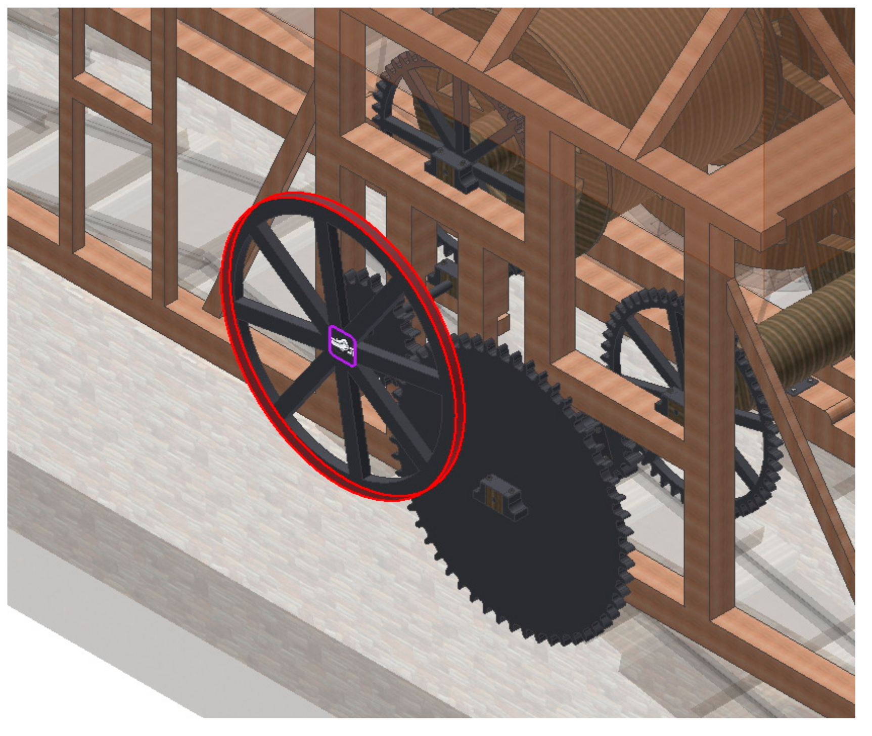
On the other hand, the rotary constraints are applied to the surfaces that rotate freely, being fundamentally the points of contact between the axles and the supports on the structure. The transmission shafts have two supports, except for the DD axle, which has the inertia flywheel. This DD axle has only one point of support, because the inertia flywheel would be linked to the inertia flywheel of the steam engine that drives it through a belt or its own support structure. For this reason, the simulation will be carried out as if the surface of the inertia flywheel also served as a rotary support. The other elements that also have surfaces that rotate freely are the contact between the pulleys and the axle on which they roll, as well as the contacts between the first parts of each brake and the axle that supports it (Figure 7).

Regarding the manual contacts, it is especially important to check that the contact between the teeth of the different gears is correctly defined. Normally, when designing and positioning the gears, the edges of the gears do not come into contact, and therefore, the static analysis can be affected. Similarly, when studying the braking position, the contact between each of the brake parts and the inertia flywheel of the axle must also be correctly defined. Thus, in all cases, the defined manual contacts are of the blocked type (Figure 8), and the rest of the contacts between elements are recognized automatically by the software.

2.2.4. Forces Applied

The definition of the forces that affect the inclined plane is perhaps the most delicate step in the preparation of the simulation, since the various parts that compose it are affected differently by different forces.

Previously, the two situations in which the mechanism will be simulated were presented: a blockage situation of the inertia flywheel, and an emergency braking situation. Both present common forces, but also different forces that will be studied in these situations.

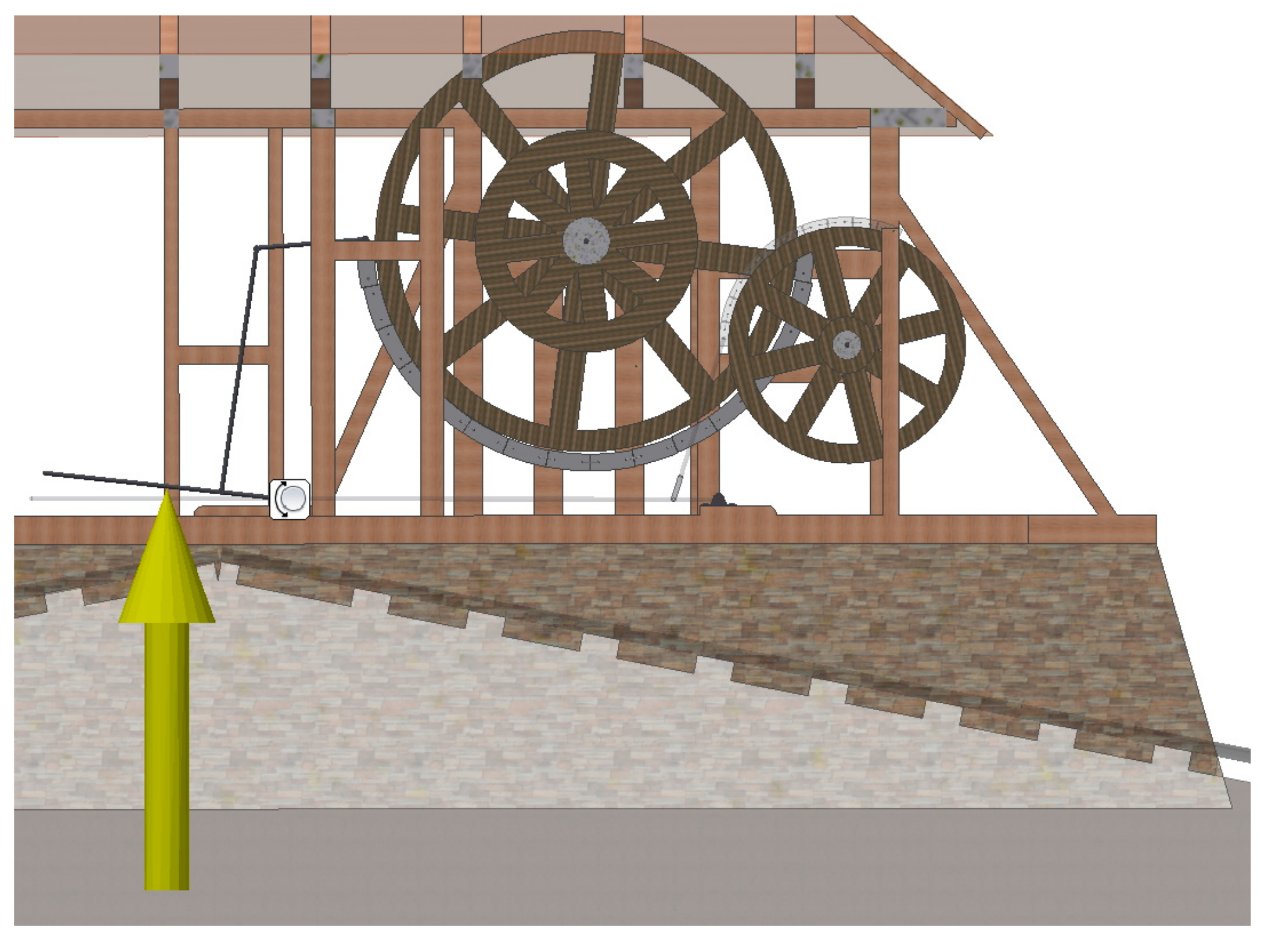
Among the forces common to both situations are the force of gravity and the tensions applied to the pulley in the direction of the rope.

Regarding gravity, the software defines it by specifying the magnitude and direction, and for it to be applied at the center of gravity of the engine, it is first delocalized by defining a generic vector of 9810 mm/s² in the direction of the Z axis in the negative direction (Figure 9).

On the other hand, there is a tension applied to the pulley through the rope, and this is due to the weight of the tugboat along with the boat. The rope embraces the pulley on the outside, and therefore, it would not be necessary to characterize this tension if the behavior of the rope was simulated. However, as explained above, the dynamic behavior of the rope prevents it from being included in the simulation, raising two questions: on the one hand, how can the tension of the rope be simulated on the outer area of the pulley?, and on the other, could the load be replaced with a torque on the pulley shaft? The answer to the first question is affirmative, but not for the second.

To be able to apply the tension on the pulley in the most realistic way, a piece of rope was taken and joined together with the pulley. On the first contact point of the pulley with the lower and upper rope, two working planes were defined in a manner transverse to the main direction of the rope. On these planes, a load equivalent to the previously calculated tension was applied (Figure 10). In addition, for each of the tensions to have the proper direction, a larger piece of rope was used, although once the loads had been defined, it was excluded from the simulation.

The two tensions have the same value, because, as will be explained later, the AA axle exerts a moment of inertia that cancels out the load of the tugboat, so the situation is static. Due to this, the value of the tension is equal to the weight of the tugboat with the boat.

According to the data provided by Betancourt, the inclined plane is 210 feet high on a plane of 880 feet in length, which translates to an angle of inclination (α) of 13.806°. Furthermore, it is considered that the mass of the boat, using the materials of the time, is M₁ = 2951.453 kg (including the trailer and the chains that rig it), and in addition it is assumed that the boat is fully loaded with a mass M₂ = 5000 kg. Therefore, the value of the tension on the rope will be:

T_rope = (M₁ + M₂) × g × sinα = 7951.453 kg × 9.81 m/s² × sin (13.806) = 18,614.44 kN

(1)

Forces at Play in the Situation of Inertia Flywheel Blockage

The calculation of the torques that cause the shafts to overcome the tension of the rope and thus to be able to raise the load on the plane is decisive. In addition, the torques of the AA and EE shafts do not have the same magnitude, since the slopes of the planes are different, although they are loaded equally. Because of this, they will be calculated independently.

The torque on the AA axle (Figure 11a) has to do with the previously calculated tension. Its calculation is very simple, since the value of the radius of the shaft drum is known, r = 1.185 m.

M_AA = T_rope × r = 18,614.44 N × 1.185 m = 22,058.11 Nm

(2)

On the other hand, the torque along the EE axle (Figure 11b) has to do with the tension supported by the tugboat rope that ascends from the upper channel. It can be assumed, in the worst case of tension, that the tugboat is also fully loaded and, therefore, that the mass is similar to the aforementioned M₁ + M₂. However, the inclination of this plane is lower than the previous one, with a value of α = 10.470°. With these data, the tension of the EE axle rope will be:

T_{rope EE} = (M₁ + M₂) × g × sin α = 7951.453 kg × 9.81 m/s² × sin (10.470) = 14,174.89 kN

(3)

Similarly, the radius of the EE axle is r = 0.3386 m, so the torque will be:

M_EE = T_{rope EE} × r = 14,174 N × 0. 3386 m = 4799.62 Nm

(4)

Finally, the inertia flywheel has to work as if it were blocked by forcing the gears in order to determine its resistance. Therefore, but only in this case, it is necessary to include a new fixed constraint to the external surface of the inertia flywheel (Figure 12).

Forces at Play in the Situation of Emergency Braking

The situation of emergency braking, in the event that the inertia flywheel of the steam engine were to break, for example, is an extreme situation that can occur, and that should be assessed for the correct dimensioning of the engine. In this case, it would only be necessary to stop the loaded tugboat that travels along the AA axle, since stopping the tugboat on the EE axle is not so important, as the distance it travels is short, and it would be immediately braked by the water of the upper channel with no danger of losing the load.

For this reason, only the torque on the AA axle, the tensions in the pulley, gravity and, finally, the brake force on the AA axle will be considered. This force has to be equivalent to the torque applied in order to be able to stop the load. Finally, in the case studied, the inertia flywheel would be released from the previously imposed fixed constraint and be able to rotate freely.

To characterize the AA axle brake, it would be necessary to study in detail the properties of the wooden brake that comes into contact with the inertia flywheel, specifically the friction coefficient of the wood. However, this coefficient changes due to a multitude of factors, such as humidity, possible surface scratching, or wear, among other causes, although an approximate value of the static friction coefficient of μ = 0.4 can be given. This value, excessively low, is of great help in calculating the force that must be exerted on the brake bar AA to stop the tugboat in the case of breakage of the transmission mechanism.

The brake consists of 16 pieces with an approximate surface area of 0.111 m² each, which means a total braking area of 1.775 m². In addition, it is known that the force that must be exerted on the perimeter of the drum must be able to cancel out the torque applied on the AA axle with a value of M_AA = 22,058.11 Nm, according to Equation (2), but on his own inertia flywheel, which has a radius of value r = 2.511 m, which is greater than the radius of the drum.

With these data, it is now possible to calculate the pressure that the brake must exert on the inertia flywheel.

P = (F/S)/µ = (M_AA/(r × S))/µ = 22,058.11 Nm/(2.511 m × 1.775 m² × 0.4) = 12,372.66 N/m²

(5)

Thus, the pressure that must be exerted is finally due to the force applied to the brake bar, and this is obtained by multiplying the calculated pressure P by the braking surface S.

F = P × S = 12,372.66 N/m² × 1.775 m² = 21,961.47 N

(6)

As can easily be verified, this force (Figure 13) is equivalent to lifting something of more than 2 tons, so the loaded tugboat could not be manually stopped with the brake alone. This makes sense, since the trailer has a mass of around 8 tons. Thus, even if the coefficients of friction were higher and the force about half, it would still be excessive to brake manually. As has been demonstrated, although William Reynolds devised a complex system of levers and articulations to decrease the force necessary to stop a tugboat that is falling freely, the force that must be exerted continues to exceed the capacity of a single human operator.

In any case, in this research, the behavior of the engine will be analyzed in a hypothetical case in which such a force could be exerted on the braking bar, although this situation would be highly unlikely.

2.2.5. Meshing

The last step before beginning the static analysis consists of the geometric discretization or meshing of the engine. Most software that performs an FEA uses tetrahedral elements, type tetra 10 (4 physical points and 10 nodes). If the simulation is more complex, for example, in dynamic analysis or in static analysis of complex geometries, some software uses hexahedral volumes, such as hexa 8, hexa 20 or hexa 27 for meshing. The use of the hexahedron allows the mesh to be formed by elements of greater volume, and therefore it needs a smaller number of elements to generate all of the geometry of the model. The choice of hexahedral meshes decreases the computational requirements and saves time, but results in less accurate results, since the total number of nodes is reduced and the mesh is less suited to the real geometry. In an analysis such as the present study, there is no problem in using tetra 10, since the total number of elements to analyze is not excessive.

Therefore, in FEA analysis, the elements used were tetrahedrons with 4 nodes and first order integration (constant interpolation of the stress and strain). The elements are formulated in a 3D scheme with three degrees of freedom per node (translational in X, Y and Z directions). However, a sensitivity analysis of the size of the element has not been carried out, since the structure is oversized.

On the other hand, the specific software used in the analysis of thermal parameters or lighting uses bar elements or shell elements. These elements of lower order than those used in the present study could also be used for the static or modal analysis of a mechanism, but it would require a much larger number of nodes to simulate its geometry, and therefore for a computer with a standard processor, these meshes would need an excessive time in their calculations. Regarding the shell elements, although they are capable of capturing the stress gradients in a more efficient way, they have not been used in this study, since the mechanism is oversized, and because it would provide an accuracy that would not change the conclusions in a significant way.

Autodesk Inventor Professional can automatically generate a mesh based on the size of the element to be discretized. By default, it generates tetrahedra whose average size is 10% of the length of the element, a minimum size of the tetrahedron of 20% of the average size, a maximum variation between tetrahedra of 1.5 and a maximum angle of rotation of 60°.

However, it is advisable to pay more attention to the places where the geometry is complex, since in these parts, the mesh usually gives results that differ greatly from the actual geometry of the element. For these singular places, the software offers the possibility of carrying out a manual meshing of the element in which the mesh size is determined. In addition, in general lines, it should be mentioned that in places where the concentration of stress is greater, it is also convenient to increase the density of the mesh. Figure 14 shows the meshing result that is generated automatically by Autodesk Inventor Professional.

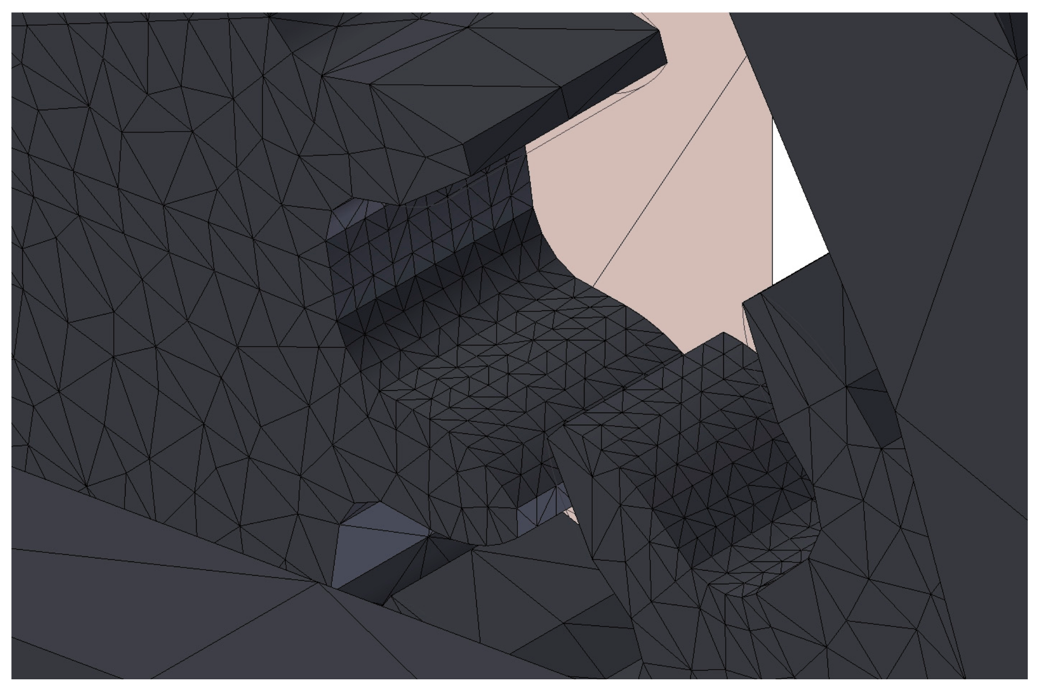
In the present research, it was also necessary to modify the discretization in some places, performing a refinement of the mesh. Specifically, this was done in the contacts between the teeth of adjacent gears (Figure 15) and on the surfaces of the ends of the axles in contact with their supports (Figure 16). In the first case, the reason for this intervention was the complicated geometry of the tooth of the gear, while in the second case, the reason lay in the concentration of the stresses.

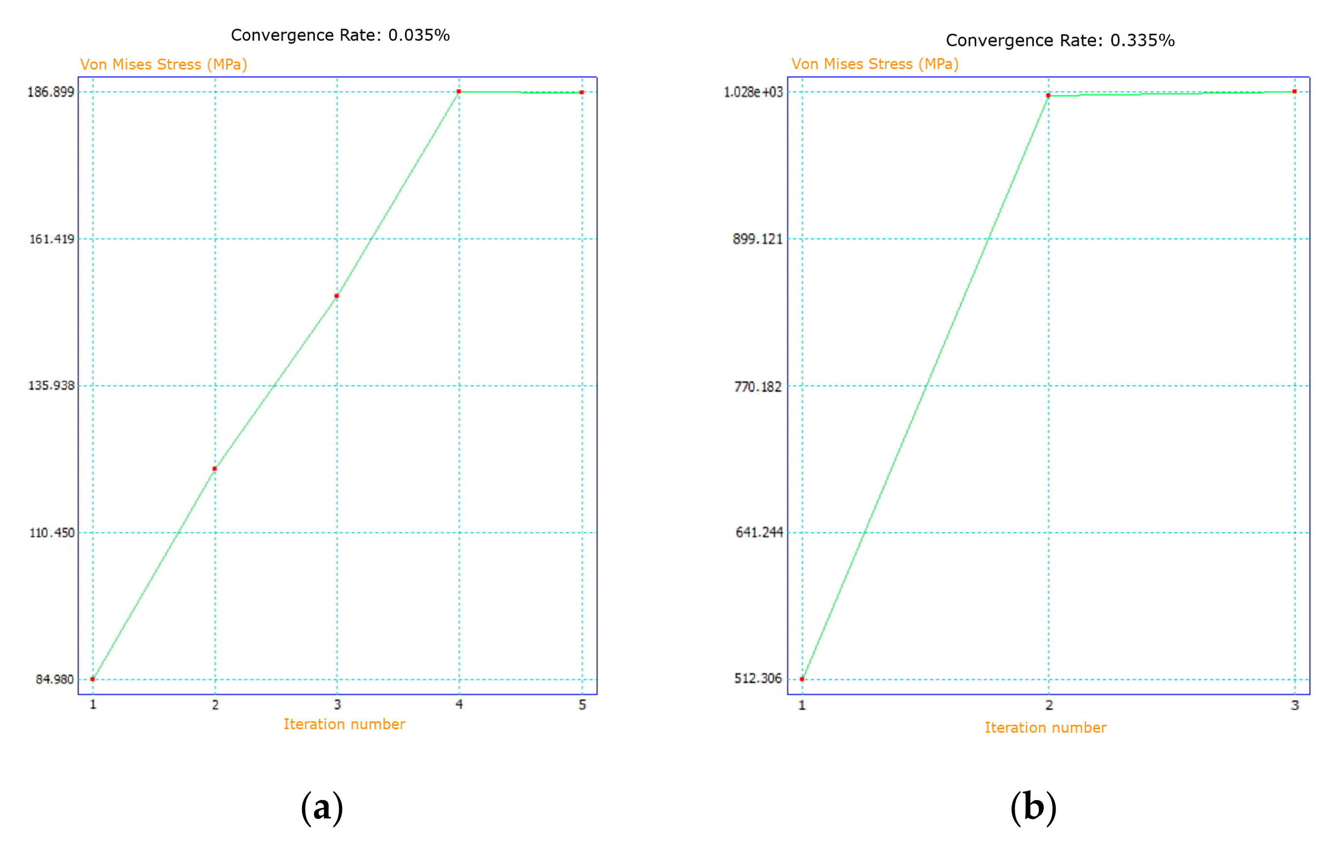
To conclude this section, it must be emphasized that for static analysis, it is necessary to establish a convergence criterion since iterative processes are used in this analysis. Thus, the result obtained is compared with the previous analysis and when it differs by less than 5% the process stops. In this research, and taking into account the computational resources available, the analysis used a mesh of 1,028,444 elements and 1,660,194 nodes in the blocking situation, and in the situation of emergency braking a mesh of 1,417,521 elements and 2,237,388 nodes.

3. Results and Discussion

On the interpretation of the results, it is convenient to point out that von Mises stresses were used instead of principal stresses. Although these show somewhat lower values than the principal stresses for the elements made of wood, it does not mean that these values are not valid, but they provide important indicative values, which, moreover, will not be too far from the value maximum stress in the most unfavorable direction.

Furthermore, the main direction of the wooden element (its greater length) is the direction parallel to the grain (the most resistant), and the engineer thought of wooden elements to work in compression. This indicative data, which shows the calculation of the von Mises stress on the wooden elements, is far from the elastic limit of the structure, whereas it shows large concentrations of stress on metal (isotropic) elements, and in this case, the von Mises stress is a precise datum of the load which the mechanism supports.

3.1. Modal Analysis

Before carrying out the static analysis, it is necessary to check previously, by means of a modal analysis, whether the engine behaves like a rigid solid. If it had such behavior, the software would provide erroneous results.

To do this, the model is subjected to a series of vibrations at different frequencies, which produces some deformations so that at high frequencies, elements appear that have a deformation greater than the reference deformation adopted by the software. Autodesk Inventor Professional provides the 8 lowest frequencies at which any part of the model is deformed, and if those frequencies are close to 0 Hz, it means that the element behaves like a rigid solid, and therefore, it would not make sense to perform a static analysis.

For the blockage situation, the following frequencies were obtained: F1: 2.00 Hz, F2: 2.81 Hz, F3: 2.83 Hz, F4: 5.78 Hz, F5: 6.25 Hz, F6: 8.11 Hz, F7: 9.00 Hz and F8: 9.04 Hz. This means that, in this situation and as expected, the model behaves statically and, therefore, the study can proceed.

For the emergency braking situation, the frequencies were different since some elements do not come into action. The results obtained were: F1: 3.39 Hz, F2: 4.25 Hz, F3: 6.37 Hz, F4: 6.42 Hz, F5: 6.71 Hz, F6: 9.08 Hz, F7: 9.26 Hz, F8: 9.46 Hz. Thus, the modal analyses of both situations were very similar without loads.

On the other hand, as explained previously, the mesh size affects the exact places where stresses are concentrated, so the software allows the possibility of establishing a study on the convergence of the results by iterating the results in the regions that are considered more convenient. Therefore, for the static analysis a maximum of 10 cycles of iteration has been established, as long as the results vary more than 5% in each iteration. If the results in a region are less than that 5%, it stops iterating. In the same way, the greater the maximum number of iterations and the smaller the variation between results, evidently, the greater the computational requirements and the more prolonged the simulation time. In any case, this study is necessary in order to obtain a reliable result.

The results of the convergence curves for the two situations studied are shown in Figure 17. In the blockage situation the convergence rate (0.035%) is reached at the fifth iteration (Figure 17a), and in the emergency braking situation, the convergence rate is lower (0.335%), reached at the third iteration (Figure 17b). Therefore, the evolution of both graphs allows us to determine that the results obtained is very reliable.

3.2. Static Analysis

As can be supposed, the results of the static analysis also vary depending on the situation in which the mechanism is studied.

In the blockage situation, the maximum stresses are located on the supports of the horizontal axles. At these points, the von Mises stress reaches a maximum at the insertion of the DD axle with the inertia flywheel with a value of 186.9 MPa (Figure 18a). Similarly, for the rest of the contacts between the axles and the supports, there also appear high stress values: the support of the AA axle is subjected to a stress of 169.5 MPa (Figure 19a), and the support of the intermediate BB axle to a stress of 77.8 MPa (Figure 20a). Outside of these points, stresses are generally low.

In the braking situation, the maximum stress is located at the point of attachment of the support bar of the first brake, with a value of 1025 MPa (Figure 18b). This stress, as was observed in the previous sections, could not be achieved, since the operator would need to use a force equivalent to 2 tons to be able to stop the loaded tugboat. Therefore, the support bar of the first brake would break. However, it should be emphasized that the rest of the structural elements would be subject to reasonable stress. Thus, the second highest stress value would be reached in the support of the bar with a value of 390.7 MPa (Figure 19b), and the third highest value (287.1 MPa), would be reached at one part of the drive shaft, and would be located at the point of contact between the shaft of the largest gear of the DD shaft and that of the BB shaft gear (Figure 20b).

Another result of the static analysis is that relative to the safety coefficient. The safety coefficient at a given point in the model is calculated as the ratio between the von Mises stress and the elastic limit of a material for that point. In other words, the safety coefficient shows graphically whether the material from which a piece is made is capable of supporting a certain stress or not. In principle, a safety factor close to one unit would indicate that the material is working very close to its elastic limit; if it is less than one, it would indicate that the material exceeds this limit and would break, and if it is greater than one, it would indicate that it works without problems when subjected to said stress.

Nowadays, the materials and their elastic limits are much better known than at the end of the 18th century, and for this reason, engineers aim for the elements to work within a range of safety coefficient of 2 to 4 units. At the time of the Hay inclined plane, on the contrary, machines tended to be oversized, since those limits were unknown. For this reason, it is not surprising that, in general, almost the entire model works well above the elastic limit of the materials.

In the blockage situation, it can be observed, however, that the axle supports work with a value of 3.51 (Figure 21a). These elements have in common that they are in contact with the most stressed elements, and therefore, William Reynolds used wooden supports, because they are elements that can be easily replaced, since there was much wear due to the excessive friction of the axles (the bearing had not yet been invented).

However, in the braking situation, the point of maximum stress (point of union of the support bar of the first brake) coincides with the one with the lowest safety factor, with a value of 0.74 (Figure 21b). Outside this bar, the points that have the lowest safety coefficient are located at the joints between the links that form the brake, with a value of 1.7 in the tenth link (Figure 22b). The rest of the links have somewhat higher values, also around 2.

Also, in the blockage situation, it must be mentioned that the union between the inertia flywheel and the axle is another delicate place. The flywheel, which is the element for which movement had been restricted, suffers an important torque in its axle. However, the safety factor of the highest stress point is 4.05, and therefore it is well dimensioned, but it is by far the point of the transmission shaft that works with the lowest safety coefficients (Figure 22a).

Finally, and also for the blockage situation, the distal support of the AA axle is shown. In this place, there is the element with the third lowest safety coefficient with a value of 4.13 (Figure 23), but already forming part of the set of oversized elements, as happens with the rest of the pieces of the mechanism.

Another aspect that static analysis studies is that of the deformations suffered by the various elements, as these play an important role in the proper functioning of the mechanism. Thus, an excessively deformed element can generate problems for the correct performance of its function, affecting the proximate elements. For example, those elements inserted in guides, crossed by bolts or those that need to keep their contacts well defined in order to gear without gaps are very sensitive to deformations.

In the blockage situation, the maximum equivalent deformation, located at the junction of the inertia flywheel with the DD axle has a value of 0.13% with respect to the size of the element, and, therefore, is negligible (Figure 24a).

However, in the braking situation (Figure 24b), the maximum equivalent deformation, located at the insertion of the braking bar with the support of the first link of the brake and according to the point of maximum stress, is somewhat greater, with a value 0.74%, although very far from representing a danger for the operation of the mechanism.

Finally, the displacements are analyzed. For reasons similar to those mentioned in the previous section, the elements subjected to a stress point can present important displacements with respect to their usual working position. However, and in general, it can be seen that most of the elements hardly suffer any displacement when subjected to normal loads.

In the blockage situation, the piece subjected to the greatest displacement, with a value of 22.98 mm, is the inertia flywheel (Figure 25a). Although this is an acceptable displacement, this data indicates again that this piece is affected by the stopping of the transmission shaft and suffers like no other the consequences of this effort. The second point where the displacement is greatest is located at a point in the structure (Figure 26a) with a value of 6.27 mm, which indicates that the displacements in the rest of the elements of the transmission shaft are negligible, and that the structure works correctly.

In the braking situation, the end of the actuated lever is the point registering the greatest displacement with a value of 247.1 mm (Figure 25b). It is a solid bar of cast iron 2 m in length, so although such a displacement is not acceptable, it is understandable given the characteristics of the force that causes it (close to 22 kN). The second maximum displacement is located at the inertia flywheel, as also happens in the blockage situation, with a value of 10.28 mm (Figure 26b). The rest of the elements present negligible displacements.

4. Conclusions

• In the present research, static analysis by FEM is shown, applied to the 3D model of the Hay inclined plane located in Coalbrookdale (Shropshire, England), the work of the English engineer William Reynolds, just as it worked a few years after its inauguration in 1792. This 3D model was developed based on the work of the Spanish engineer Agustín de Betancourt, who published a report about the method used by Reynolds to negotiate uneven channels using inclined planes. For these tasks, Autodesk Inventor Professional software was used.
• Static analysis was used to study the behavior of the engine in the two most unfavorable situations: the first one, in which a inertia flywheel blockage due to a problem in the steam engine is simulated, and a second one in which emergency braking of a loaded tugboat is required by the disconnection between the inertia flywheel and the steam engine.
• The results of the static analysis were very different, depending on the situation analyzed. For the blockage situation, a maximum stress of 186.9 MPa was obtained at the insertion point of the inertia flywheel with the DD axle. In addition, the wooden support of said DD axle had the lowest safety coefficient with a value of 3.51, which indicates that it is well dimensioned. The same DD axle would have a negligible maximum deformation of 0.13%, and the maximum displacement is located at the inertia flywheel, with a value of 22.98 mm. Similarly, it was observed that the rest of the elements always had values on the side of safety, so for this situation, it can be said that the mechanism is oversized; that is, the materials work far below their elastic limit, just as happened in the designs of the time.
• However, the results were different in the emergency braking situation. On the one hand, as stated above, this second situation, although it would be highly advisable in the face of an emergency situation, was impossible to resolve in practice. That is, unless there was a mechanical system for actuating the lever (which is not described in the written account, but would certainly have existed), it would be impossible to exert sufficient braking pressure using human means. As was seen, the force that it would be necessary to exert on the brake bar to stop the mechanism was almost 22 kN, very far beyond the capacity of a human operator. In any case, it was considered useful to approach the study of this hypothetical situation as a method for evaluating the mechanism structurally.
• Also, the static analysis of this emergency braking situation was very revealing. For this situation, a maximum stress of 1025 MPa is reached at the point of insertion of the brake bar and the first link of the brake, and since the elastic limit of cast iron is 758 MPa, at that point the bar would break. In addition, the security coefficient at this point is 0.74, confirming, therefore, the invalidity of its dimensions. However, the analysis is surprising for two reasons: on the one hand, a low security coefficient is not necessarily excessive, so a simple change in the dimensions of the bar would be enough for this element to fall within the safety range; and on the other hand, it is striking that it is the only point where these values are exceeded. The second maximum stress is located at the insertion point of the braking bar with its support presenting an acceptable value of 390.7 MPa, and the second point with the lowest safety coefficient corresponds to the links that join the brake parts with a value of 1.7, which falls within the safety range. As indicated above, although this emergency braking situation could not occur manually, it is verified that for such a large braking stress the structure would function correctly except in the dimensioning of the braking bar. In fact, this bar is the element where the greatest equivalent deformation and the largest displacement within the mechanism is located, with values of 0.73% and 247.1 mm, respectively. The latter value would suggest the need for a resizing of the bar.
• All these data show that by the time it was built, the invention was correctly sized. The hypothesis of work in the situation of emergency braking indicates, on the other hand, that it would be difficult to stop a loaded tugboat using the axle brake (which would entail a certain danger for loads and people), but at the same time, it shows that, despite this, the general structure (except for the braking bar) was well dimensioned. The Hay inclined plane was in operation from 1792 to 1944, and this fact corroborates all the results shown here. At the same time, the present research emphasizes that, from the point of view of mechanical design, the invention of William Reynolds has all the qualities to qualify it as a ‘masterpiece’.

References

1. Muñoz Bravo, J. Biografía Cronológica de Don Agustín de Betancourt y Molina en el 250 Aniversario de su Nacimiento; Acciona Infraestructuras: Murcia, Spain, 2008. (In Spanish) [Google Scholar]
2. Martín Medina, A. Agustín de Betancourt y Molina; Dykinson: Madrid, Spain, 2006. (In Spanish) [Google Scholar]
3. Cioranescu, A. Agustín de Betancourt: Su Obra Técnica y Científica; Instituto de Estudios Canarios: La Laguna de Tenerife, Spain, 1965. (In Spanish) [Google Scholar]
4. Rojas-Sola, J.I.; Galán-Moral, B.; De la Morena-De la Fuente, E. Agustín de Betancourt’s double-acting steam engine: Geometric modeling and virtual reconstruction. Symmetry 2018, 10, 351. [Google Scholar] [CrossRef]
5. Rojas-Sola, J.I.; De la Morena-de la Fuente, E. Digital 3D reconstruction of Agustín de Betancourt’s historical heritage: The dredging machine of the port of Krondstadt. Virtual Archaeol. Rev. 2018, 9, 44–56. [Google Scholar] [CrossRef]
6. Rojas-Sola, J.I.; De la Morena-de la Fuente, E. Geometric modeling of the machine for cutting cane and other aquatic plants in navigable waterways by Agustín de Betancourt y Molina. Technologies 2018, 6, 1. [Google Scholar] [CrossRef]
7. Rojas-Sola, J.I.; De la Morena-de la Fuente, E. Agustín de Betancourt’s wind machine for draining marshy ground: Approach to its geometric modeling with Autodesk Inventor Professional. Technologies 2017, 5, 2. [Google Scholar] [CrossRef]
8. Rojas-Sola, J.I.; De la Morena-De la Fuente, E. Agustín de Betancourt’s mechanical dredger in the port of Kronstadt: Analysis through Computer-Aided Engineering. Appl. Sci. 2018, 8, 1338. [Google Scholar] [CrossRef]
9. Rojas-Sola, J.I.; De la Morena-De la Fuente, E. Agustín de Betancourt’s double-acting steam engine: Analysis through Computer-Aided Engineering. Appl. Sci. 2018, 8, 2309. [Google Scholar] [CrossRef]
10. Rojas-Sola, J.I.; De la Morena-De la Fuente, E. Agustín de Betancourt’s wind machine for draining marshy ground: Analysis of its Construction through Computer-Aided Engineering. Inf. Constr. 2018, 70, e236. [Google Scholar] [CrossRef]
11. Rojas-Sola, J.I.; De la Morena-De la Fuente, E. Agustín de Betancourt’s piston lock: Analysis of its Construction through Computer-Aided Engineering. Inf. Constr. 2019, 71, e286. [Google Scholar] [CrossRef]
12. Rojas-Sola, J.I.; De la Morena-De la Fuente, E. Agustín de Betancourt mil for grinding flint: Analysis by Computer-Aided Engineering. Dyna 2018, 93, 165–169. [Google Scholar] [CrossRef]
13. Rojas-Sola, J.I.; De la Morena-De la Fuente, E. The Hay inclined plane in Cooalbrookdale (Shropshire, England): Geometric modeling and virtual reconstruction. Symmetry 2019, 11, 589. [Google Scholar] [CrossRef]
14. Hadfield, C. Thomas Telford’s Temptation; M. & M. Baldwin: Cleobury Mortimer, UK, 1993. [Google Scholar]
15. Betancourt, A. Dessin de la Machine Pour Faire Monter et Descendre les Bateaux d’un Canal Inferieur a un Superieur et Reciproquement Sur Deux Plans Inclines. Available online: http://fundacionorotava.org/pynakes/lise/betan_dessi_fr_01_179X/0/?zoom=large (accessed on 15 August 2019).
16. Betancourt, A. Mémoire Sur un Nouveau Système de Navigation Intérieure. Available online: http://fundacionorotava.es/pynakes/lise/betan_memoi_fr_01_1807 (accessed on 15 August 2019).
17. Fulton, R. A Treatise on the Improvement of Canal Navigation; I. and J. Taylor: London, UK, 1796. [Google Scholar]
18. Hay Inclined Plane (from the Bottom Canal) in 1879. Available online: https://captainahabswaterytales.blogspot.com/search?q=hay+plane (accessed on 15 August 2019).
19. Hur, D.J.; Know, S. Fatigue analysis of greenhouse structure under wind load and self-weight. Appl. Sci. 2017, 7, 1274. [Google Scholar] [CrossRef]
20. Li, J.B.; Gao, X.; Fu, X.A.; Wu, C.L.; Lin, G. A nonlinear crack model for concrete structure based on an extended scaled boundary finite element method. Appl. Sci. 2018, 8, 1067. [Google Scholar] [CrossRef]
21. Fundación Canaria Orotava de Historia de la Ciencia. Available online: http://fundacionorotava.org (accessed on 15 August 2019).
22. Proyecto Betancourt. Available online: http://fundacionorotava.es/betancourt (accessed on 15 August 2019).
23. Shih, R.H. Parametric Modeling with Autodesk Inventor 2016; SDC Publications: Mission, KS, USA, 2015. [Google Scholar]
Figure 1. Isometric view of the Hay inclined plane.
Applsci 09 03385 g001
Figure 2. Plan of the ensemble with an indicative list of the different elements.
Applsci 09 03385 g002
Figure 3. Detail of the transmission trees and gears of the engine.
Applsci 09 03385 g003
Figure 4. Sequence of movements in the ascent of the tugboats.
Applsci 09 03385 g004
Figure 5. Simplified model of the Hay inclined plane for static analysis.
Applsci 09 03385 g005
Figure 6. Fixed constraints applied: (a) support of the support structure (b) support of the BB shaft.
Applsci 09 03385 g006
Figure 7. Rotary supports.
Applsci 09 03385 g007
Figure 8. Manual contact defined between gears.
Applsci 09 03385 g008
Figure 9. Gravitational force applied at the center of gravity of the engine.
Applsci 09 03385 g009
Figure 10. Forces applied on the pulley in the direction of the rope.
Applsci 09 03385 g010
Figure 11. (a) Torques applied on the AA shaft and (b) on the EE shaft.
Applsci 09 03385 g011
Figure 12. Fixed constraint for the inertia flywheel of the DD shaft in the blockage situation.
Applsci 09 03385 g012
Figure 13. Force exerted on the braking bar in the situation of emergency braking.
Applsci 09 03385 g013
Figure 14. Automatic mesh obtained from the Hay inclined plane.
Applsci 09 03385 g014
Figure 15. Refinement of the mesh in the teeth of the gears.
Applsci 09 03385 g015
Figure 16. Refinement of the mesh at the ends of the shafts in contact with the supports.
Applsci 09 03385 g016
Figure 17. Convergence curve: (a) blockage situation and (b) braking situation.
Applsci 09 03385 g017
Figure 18. Location of the highest von Mises stress: (a) blockage situation and (b) braking situation.
Applsci 09 03385 g018
Figure 19. Location of the second highest von Mises stress: (a) blocking situation and (b) braking situation.
Applsci 09 03385 g019
Figure 20. Location of the third highest von Mises stress: (a) blocking situation and (b) braking situation.
Applsci 09 03385 g020
Figure 21. Location of the lowest safety coefficient: (a) blockage situation and (b) braking situation.
Applsci 09 03385 g021
Figure 22. Location of the second lowest safety coefficient: (a) blockage situation and (b) braking situation.
Applsci 09 03385 g022
Figure 23. Third lowest safety coefficient in the blockage situation.
Applsci 09 03385 g023
Figure 24. Location of the highest deformation: (a) blockage situation and (b) braking situation.
Applsci 09 03385 g024
Figure 25. Location of the highest displacement: (a) blockage situation and (b) braking situation.
Applsci 09 03385 g025
Figure 26. Location of the second highest displacement: (a) blockage situation and (b) braking situation.
Applsci 09 03385 g026