Research on an Output Power Model of a Doubly-Fed Variable-Speed Pumped Storage Unit with Switching Process

Abstract

The doubly-fed variable-speed pumped storage (DFVSPS) is an effective method to balance the fluctuation of renewable energy generation and is an important means of frequency and voltage regulation of a power grid. Firstly, this paper introduces the structure and mathematical model of the DFVSPS unit. Secondly, the control methods of each switching stage in generating mode and pump mode are proposed, and the simulation study of each stage of DFVSPS switching process is carried out by MATLAB/Simulink. Thirdly, when studying the regulating effect of DFVSPS unit in the power system, due to the high switching frequency of converter in the electromagnetic transient model, the simulation speed is very slow and the data volume is large, so the model of DFVSPS unit needs to be simplified. By analyzing the dynamic behavior of the pumped storage power station, the mathematical model of output power of the DFVSPS unit is established, which includes start-up stage, load ramping stage, stable operation stage, load rejection stage and shutdown stage of generating mode and pump mode. Finally, the simplified model of DFVSPS unit is applied to a simple power system to verify its regulating effect on grid power.

1. Introduction

Power balance is the foundation of stable operation of a power system, and the frequency and voltage of a power system must be maintained within a certain range to maintain the balance of active power and reactive power. However, with the increase in the proportion of a large-capacity rigid power supply such as nuclear power, and the large-scale development of renewable energy generation, the power balance of a power system is confronted with great challenges [1,2]. The power balance of a power system can be realized through the power absorption and emission of an energy storage system, which is an important way to keep the system running smoothly [3].

A pumped storage power station is an important method of energy storage. It has functions such as peak load shifting, frequency modulation and accident standby [4]. Compared with traditional fixed-speed pumped storage unit, the variable-speed pumped storage unit can adjust the speed according to the change of the head under generating mode, which can improve its operating efficiency and can adjust its power under pump mode, which has a wider range of adjustment, faster adjustment speed and better adjustment effect [5,6]. Therefore, research on switching process and the dynamic response of a pumped storage power station is significant for the power grid to rationally use the functions of a pumped storage power station.

Currently, the research on the transition process of DFVSPS unit mainly focuses on the performance research of the pump turbine system when the unit is in a bad working condition, such as the sudden power failure of the pump mode and the 100% load rejection of generating mode. The main purpose of these studies is to improve the operating performance of units during tough conditions. As shown in Ref. [7], transient characteristics during the closure of guide vanes in a pump-turbine in pump mode were studied. In Refs. [8,9], the S-shaped region of pump turbine was analyzed. Flow characteristics of the transient power interruption process of a prototype pump-turbine at pump mode were studied in Ref. [10], and flow analysis of pump turbine in load rejection was mentioned in Ref. [11]. However, these studies are only focused on the unit itself and do not take into account the requirements of the power system on the unit’s operational performance.

For the application research of the DFVSPS unit in the power system, the current research is mainly on the combined operation of pumped storage system and photovoltaic, wind power, etc., to reduce the fluctuation of wind power and photovoltaic output. There is also literature on the power output characteristics of DFVSPS units in the stable operation stage. In Ref. [12], the coordinated control of wind turbine and pumped storage unit were studied, and pumped storage unit and photovoltaic power generation system in Refs. [13,14,15] carried out modelling and static analysis on the stable operation stage of DFVSPS unit. Ref. [16] reviewed the converters used in DFVSPS units. However, the above literature only shows that the DFVSPS units have the compensation ability for power fluctuations, but the compensation range and compensation speed are not studied.

Therefore, it is of great significance for DFVSPS units to exert their advantages, suppress the fluctuation of output and enhance the reliability of the power system to research the influence of the DFVSPS units on the power system in the transition process, study the compensation range and compensation speed of the DFVSPS units for power fluctuation, and established a power output model based on unit parameters and control parameters of DFVSPS units.

In the second part of the paper, the mathematical model of each part of the DFVSPS unit is established. The control methods of start-up stage, load ramping stage, stable operation stage, load rejection stage and shutdown on generating mode and pump mode of DFVSPS unit are analyzed in the third part of the paper, and each stage is simulated in MATLAB/Simulink; the converter switching frequency is up to 2–10 kHz, and there will be problems such as slow simulation speed and large amount of data. Therefore, in the fourth section of this paper, the power output model of the DFVSPS unit to the grid is simplified, and the simulation effect and simulation time are compared with the electromagnetic transient model. Finally, the simplified power model is applied to a three-machine system to verify the correctness of the conclusion.

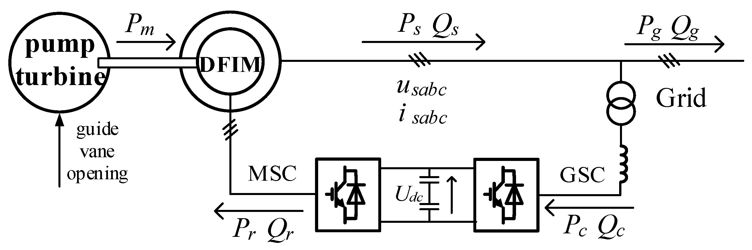
2. The Composition and Mathematical Model of Doubly-Fed Variable-Speed Pumped Storage Units

The doubly-fed variable speed pumped storage unit is composed of reversible pump turbine, doubly-fed induction motor (DFIM), converter and control part. The pump turbine provides or consumes power as a prime mover or load. The stator of DFIM is the same as that of a traditional salient-pole synchronous motor. The rotor has symmetrical three-phase windings, which are connected to the grid through the converter to exchange power with the grid. The amplitude, frequency and phase of the voltage or current output by the converter are controlled by an excitation regulator. The structure diagram of the DFVSPS is shown in Figure 1.

GSC is grid side converter; MSC is machine side converter; P_m is the mechanical power; P_s, Q_s are the active power and reactive power of DFIG stator side, respectively; P_r, Q_r are the active power and reactive power of the DFIG rotor side, respectively; P_c, Q_c are the active power and reactive power of the grid flow to the converter, respectively; P_g, Q_g are the active power and reactive power of the DFVSPS unit flow to the grid, respectively; U_dc is the direct current bus voltage of converter.

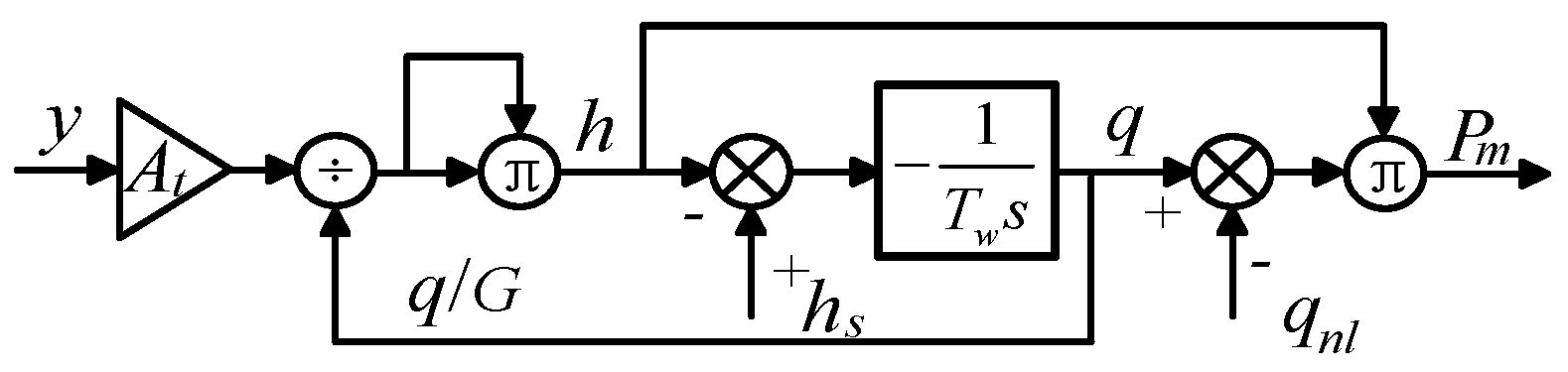
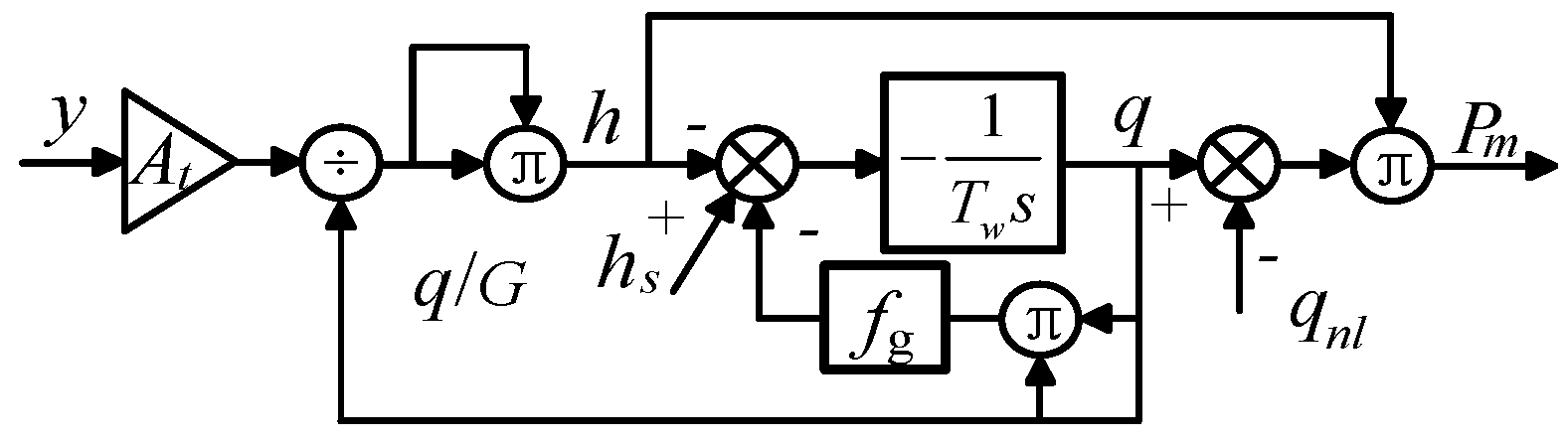
2.1. Mathematical Model of the Reversible Pump-Turbine

When the output power of DFVSPS unit is continuously adjusted, the speed of the unit will fluctuate constantly. Therefore, the regulating system is required to make the pump turbine adapt to the fluctuations of output power and adjust the speed to stabilize near the speed reference. The pump turbine regulating system is mainly comprised of a governor, electro-hydraulic servo system, DFIM, pump turbine and water diversion system, and the connection diagram of each part is shown in Figure 2.

n is the speed of DFVSPS unit; n_ref is the speed reference of DFVSPS unit; T_m is mechanical torque; T_e is electromagnetic torque.

The mainstream proportion integration differentiation (PID) governor is adopted in the governor part. The PID governor has the advantages of being easy to use, strong stability and good robustness, and can be adjusted according to the deviation between the given reference value and the actual value. The function of the electro-hydraulic servo system is to convert the electrical signal of the governor into a mechanical signal for output, thereby controlling the guide vane opening. When an ac servo motor/electro-hydraulic actuator is used in the electro-hydraulic servo system, shown in Figure 3, in order to simplify the model for the convenience of research, the nonlinear links such as saturation limiting of a servomotor, dead zone and gap nonlinearity are ignored, and the linear transfer function can be simplified into the form shown in Formula (1).

Where: y_pid is the output guide vane opening of governor; y is the output guide vane opening of servo system; y₁ is the output guide vane opening of AC servo mechanism. There is a dead zone of governor output and a saturation limiting of main servomotor. T_y1 is the AC servo mechanism response time constant; T_y is the main servomotor time constant:

$$\frac{y(s)}{y_{pid}(s)}=\frac{1}{T_{y}s(T_{y1}s+1)+1}.$$

(1)

The rigid water hammer model is adopted for a water traced pipeline, and the dynamic equation of the water traced pipeline can be expressed by Formula (2):

$$\frac{H(s)}{Q(s)}=-T_{w}s,$$

(2)

where: H is the head of pump turbine; Q is the water flow of pump turbine; T_w is water flow inertia time constant.

The structure of the pump turbine is complex, the operating conditions change frequently during the operation, the internal flow field is complex, and it is affected by the effects of water hammer, water guiding mechanism and cavitation erosion, etc. For the internal characteristics of the pump turbine, many internal fluid factors need to be considered, so it is difficult to get a mathematical model consistent with the actual situation. The pump turbine model is generally expressed quantitatively through a model test. The model test is to carry out the simulation test on the experimental table according to the actual possible various conditions (including the switching process), and record the relevant data to form the full characteristic curve. The full characteristic curve contains all features of the pump turbine during the operation process. Using the full characteristic curve to study the switching process of pump turbine is now a common method. The full-characteristic curve of pump-turbine obtained by the model test method is shown in Figure 4.

In Figure 4, the red line indicates the path of the pump turbine switching process, and numbers in Figure 4 indicate the various stages of the switching process. The details will be described later.

The mechanical torque T_m of the pump turbine and the flow Q are related to the guide vane opening y, head H, and the rotational speed n, and the relationship between them can be expressed by Formula (3):

$$\{\begin{array}{l}{T}_m=T_m\left(y,H,n\right)\\ Q=Q\left(y,H,n\right)\end{array}.$$

(3)

Different pump turbine models can be obtained by analyzing Equation (3) with different methods. In order to simplify the calculation, the pump turbine model is divided into two parts: the turbine operating condition model and the pump operating condition model.

The characteristic curve of pump turbine during its turbine operating condition is similar to the conventional turbine in the low speed region [17], as shown in Figure 5. Since the transition process in this paper is the transition process during the normal operation of the unit, all in the low speed region, so the model of the conventional turbine can be used to replace the model of pump turbine under turbine operating conditions.

The conventional turbine mathematical model commonly used at present is a simplified nonlinear model, which has a simple structure and can better reflect the fluid characteristics inside the turbine [18]. This model is proposed by IEEE [19] and the nonlinear turbine model can be expressed as Formula (4) in case of the loss of water head is ignored:

$$\{\begin{array}{l}q=A_{t}y\sqrt{h}\\ P_m=(q-q_{nl})h\end{array},$$

(4)

where: q is the flow; y is the ideal guide vane opening; h is the head; A_t = 1/(y_FL − y_NL), y_FL is an ideal guide vane opening; y_NL is the no-load guide vane opening; P_m is the mechanical power; q_nl is the no-load flow. Each variable in the model of pump turbine is represented by the per unit value (taking the rated value of the unit as the base value). When connected with DFIM, the output of pump turbine needs to be converted to an actual value.

The block diagram of this model using the rigid water hammer in Formula (2) is shown in Figure 6.

Where G is the actual guide vane opening and h_s is the static head of water.

The mathematical model of the pump turbine under pump condition is: according to the full characteristic curve of the pump turbine in the positive pump area, it can be found that, when the guide vane opening is small, the guide vane opening can regulate the flow of a pump turbine. However, after the guide vane opening becomes larger, the flow curves corresponding to different guide vane opening coincide with each other. Therefore, in the area of large guide vane opening, the guide vane opening has no obvious adjustment effect on the flow. At this time, there is an obvious regulating relationship between the speed and the flow of the unit. Therefore, the model of the pump turbine under pump mode can be divided into two parts: the pump mode model in small guide vane opening and the pump mode model in large guide vane opening. According to the relevant literature [20,21], different pump turbine, different guide vane opening of the characteristics curves start to coincide seriously. In general, the DFVSPS unit enters the stable operation stage when the guide vane opening is about 50% under start-up stage in pump mode.

Pump mode model under small guide vane opening is consistent with turbine operation mode, except that the direction of water flow is opposite to the turbine operation mode. When the pump turbine operates at small guide vane opening in pump mode, and the head loss increases sharply, which will have a great impact on the torque and flow of the pump turbine. Therefore, the head loss caused by the change of guide vane opening needs to be taken into account at this time. The pump mode model under small guide vane opening is shown in Figure 7.

Where the other quantities are consistent with generating mode, f_g is the head loss coefficient, f_g = (G_max − G)/G, and G_max is the maximum guide vane opening.

Pump mode model under large guide vane opening: according to the full characteristic curve and the related literature under the large guide vane opening of the positive water pump area of the pump turbine [22], the characteristics of the pump turbine can be expressed by Formula (5).

$$\frac{Q_1}{Q_2}=\frac{n_1}{n_2}, \frac{H_1}{H_2}={(\frac{n_1}{n_2})}^2, \frac{P_{m1}}{P_{m2}}={(\frac{n_1}{n_2})}^3$$

(5)

where subscript 1, 2 indicates working points at two different speeds.

2.2. Model of DFIM

For the convenience of analysis and control, the model of DFIM in three static coordinate systems is transformed into the model of two-phase rotating coordinate system by using the constant amplitude transformation. In addition, the nonlinear strongly coupled system is converted into linear decoupling system [23,24,25].

Voltage equation

$$\{\begin{array}{l}{u}_{sd}=R_s{i}_{sd}+p{\Psi }_{sd}-{\omega }_s{\Psi }_{sq}\\ u_{sq}=R_s{i}_{sq}+p{\Psi }_{sq}+{\omega }_s{\Psi }_{sd}\\ u_{rd}=R_r{i}_{rd}+p{\Psi }_{rd}-s{\omega }_s{\Psi }_{rq}\\ u_{rq}=R_r{i}_{rq}+p{\Psi }_{rq}+s{\omega }_s{\Psi }_{rd}\end{array}$$

(6)

where u_sd, u_sq, u_rd and u_rq are the d, q-axis voltage of stator and rotor; i_sd, i_sq, i_rd and i_rq are the d, q-axis current of stator and rotor; ψ_sd, ψ_sq, ψ_rd and ψ_rq are the d, q-axis flux linkage of stator and rotor; R_s, R_r are the resistance of stator and rotor; p is Laplace operator; ω_s is synchronous speed of DFIM; s is the slip of DFIM.

Flux equation

$$\{\begin{array}{l}{\Psi }_{sd}=L_s{i}_{sd}+L_m{i}_{rd}\\ {\Psi }_{sq}=L_s{i}_{sq}+L_m{i}_{rq}\\ {\Psi }_{rd}=L_m{i}_{sd}+L_r{i}_{rd}\\ {\Psi }_{rq}=L_m{i}_{sq}+L_r{i}_{rq}\end{array},$$

(7)

where L_s, L_r are the inductance of stator and rotor; L_m is the mutual inductance.

Electromagnetic torque equation

$$T_e=\frac{3}{2}{p}_n{L}_m(i_{sq}{i}_{rd}-i_{sd}{i}_{rq}),$$

(8)

where p_n is the number of poles.

Motion equation

$$\frac{J}{p_n}\frac{d{\omega }_m}{dt}=T_e-T_m-B_m{\omega }_m,$$

(9)

where ω_m is speed of DFIM; J is rotational inertia of DFIM; B_m is friction coefficient of DFIM.

For the convenience of analysis and control, voltage oriented vector control strategy is adopted, and then:

$$\{\begin{array}{l}{u}_{sd}=U_s\hfill \\ u_{sq}=0\hfill \end{array},$$

(10)

where U_s is effective value of grid voltage.

When the influence of resistance and the dynamic change process of flux on the transition process is ignored, the relationship between the quantities is derived, and:

$$\{\begin{array}{l}{P}_s=\frac{3}{2}(u_{sq}{i}_{sq}+u_{sd}{i}_{sd})=-\frac{3}{2}\frac{L_m{U}_s}{L_s}{i}_{rd}\hfill \\ Q_s=\frac{3}{2}(u_{sq}{i}_{sd}-u_{sd}{i}_{sq})=\frac{3}{2}{U}_s[\frac{U_s}{L_s{\omega }_s}+\frac{L_m}{L_s}{i}_{rq}]\hfill \end{array},$$

(11)

$$T_e=\frac{3}{2}{p}_n{L}_m(i_{sq}{i}_{rd}-i_{sd}{i}_{rq})=-\frac{3}{2}\frac{p_n{U}_s{L}_m}{L_s{\omega }_s}{i}_{rd}.$$

(12)

Decoupling control of active power and reactive power of DFIM is realized.

The values of the parameters of DFIM in this paper are shown in

Table 1. Parameters of DFIM.

Parameters	Value	Parameters	Value
rated power	300 MW	stator resistance Rs	0.00103 Ω
frequency	50 Hz	rotor resistance Rr	0.00065 Ω
rated voltage	18 kV	stator inductance Ls	0.000194 H
inertia J	4,000,000 kg·m2	rotor inductance Lr	0.000267 H
pole pairs p	12	mutual inductance Lr	0.00567 H

.

3. Control Method and Control Characteristics of the Switching Process of the DFVSPS Unit

Generally speaking, pumped storage power stations have static standby mode, generating mode, pump mode, and synchronous condenser operation. The common switching process is the switching between static standby mode, generating mode and pump mode. The conventional switching process consists of start-up, load ramping, stable operation, load rejection and orderly shutdown [26]. The expression of main switching process path in the full characteristic curve is shown in Figure 4—in which, $①$ is the path of the start-up stage in generating mode; $②$ is the path of the load ramping stage in generating mode; $③$ is the path of the stable operation stage in generating mode and $④$ is the path of the load rejection stage in generating mode. $⑤$ is the path of the start-up stage in pump mode; $⑥$ is the path of the load ramping stage in pump mode; $⑦$ is the path of the stable operation stage in pump mode and $⑧$ is the path of the load rejection stage in pump mode.

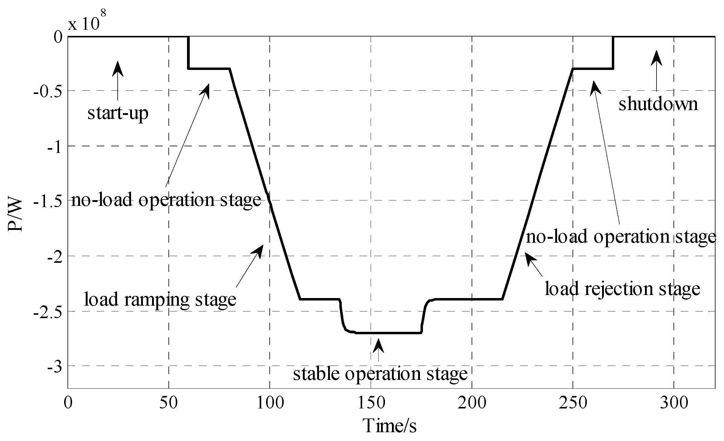
3.1. Generating Mode

The switching process of generating mode can be divided into start-up, load ramping, stable operation, load rejection, orderly shutdown and other stages. From the switching process in the full characteristic curve, the start-up is mainly to load the unit speed to the synchronous speed and complete voltage regulation and grid connection. In the stage of load ramping, the output power of the unit is increased from no-load power to full power by adjusting guide vane opening. Stable operation stage refers to the high efficiency operation of the unit near the rated operating point. The load rejection stage is mainly to regulate the unit from full power to no-load power by adjusting guide vane opening. Orderly shutdown refers to the stage when the unit is disconnected from the power grid, the unit speed drops to 0, and the unit turns to static standby. The control method is described in stages.

3.1.1. Start-Up in Generating Mode

There are two ways to start a DFVSPS unit in generating mode. The following is illustrated by combining the motion equation of DFIM shown in Formula (9).

Method 1: Start-up using mechanical torque. At this time, the rotor side of DFIM in not controlled, and the stator side of DFIM is short-circuited by three phases, so T_e = 0. Open the guide vane opening and start using the mechanical torque of pump turbine. Regarding the setting of the guide vane opening at the time of start-up, one method is to set the guide vane opening to the no-load guide vane opening (about 5% or so) until the unit is accelerated to the rated speed and then connected to the grid. Another method is to first open the guide vane opening to a larger guide vane opening to shorten the start-up time of the unit, and then reduce the guide vane opening to the no-load guide vane opening after the speed reaches a certain set value. In addition, connect to the grid until the speed reaches the rated speed.

Method 2: Start-up using electromagnetic torque. At this time, the stator of DFIM is short-circuited in three phases. Electromagnetic torque is generated by the excitation control system on the rotor side of DFIM. After the unit accelerated to the rated speed, the control strategy of the excitation control system is changed for grid connection.

Method one is used to start the unit in this paper. The rotor side of DFIM is not controlled, the stator side of DFIM is short circuited in three phases, and the guide vane opening is opened to the no-load guide vane opening, which is 6% until the speed rises to the rated speed. The simulation model was established in MATLAB/Simulink (version, Manufacturer, City, US State abbrev, USA) (The values of the parameters of DFIM in this paper are shown in Table 1 and other value of parameters used in this paper are T_w = 0.5, T_y1 = 0.07, T_y = 1, h_s = 1, q_nl = 0, A_t = 1, G_max = 1), start-up in generating mode was simulated, and the following simulation waveform could be obtained (The positive direction of each power is subject to the power in generating mode, as shown in Figure 1. The speed direction in the generating mode is specified as positive direction of speed).

According to Figure 8, the guide vane opening and mechanical power of pump turbine remain constant during the whole start-up stage. In addition, the speed of unit slowly increased to the synchronous speed.

3.1.2. Voltage Regulation and Grid Connection

After the DFVSPS unit started in generating mode and the speed reached the rated speed, the voltage on the stator side of the DFIM needs to be adjusted to meet the grid-connected conditions. When grid connection is performed, the magnitude, frequency, phase and phase sequence of the voltage on the stator side of DFIM are required to be the same as the grid voltage [27].

Before the grid connection, the stator side of DFIM is open, and the current on the stator side is 0. Thus, i_sd = 0, i_sq = 0, T_e = 0. Substituting this constraint relationship into the stator and rotor flux equation and the voltage equation, Formula (13) can be obtained:

$$\{\begin{array}{l}{U}_{sd}=\frac{d{\psi }_{sd}}{dt}-{\omega }_1{\psi }_{sq}=L_m\frac{d{i}_{rd}}{dt}-{\omega }_1{L}_m{i}_{rq}\\ U_{sq}=\frac{d{\psi }_{sq}}{dt}+{\omega }_1{\psi }_{sd}=L_m\frac{d{i}_{rq}}{dt}+{\omega }_1{L}_m{i}_{rd}\end{array}.$$

(13)

When grid voltage orientation is used and the stator resistance is ignored, U_sd = U_s, U_sq = 0. Since the dynamic performance of the stator side is not highly required during the grid-connecting process, the dynamic process of the flux linkage is neglected, and the stator-side voltage equation can be further simplified and the following relationship can be obtained:

$$\{\begin{array}{l}{i}_{rd}=0\hfill \\ i_{rq}=-\frac{U_s}{{\omega }_1{L}_m}\hfill \end{array}.$$

(14)

The above formula indicates that the voltage on the stator side of DFIM can be adjusted by regulating the q-axis current to reach the grid-connected conditions. The simulation is performed in MATLAB/Simulink, and the waveform is shown in Figure 9. The unit is connected to the grid at t = 90.4 s. In addition, it can be found that the voltage difference before the grid connection is very small.

3.1.3. On-Grid Operation Stage

After grid connection, the DFVSPS unit is in the grid-connected operation state. There are two control methods when the DFVSPS unit in the grid-connected operation stage, which are power priority control strategy and speed priority control strategy. According to the research of related literatures, the power priority control strategy has better control characteristics when realizing power control of unit features, while the speed priority control strategy has an advantage in speed regulation. In the research of this paper, the power of the unit should be controlled whether it is in the load ramping stage, load rejection stage or the stable operation stage. Therefore, the power priority control strategy is adopted. The overall control strategy diagram is shown in Figure 10.

The grid-side converter implements dc voltage control, the rotor-side converter realizes the control of the power, and the guide vane opening control system of pump-turbine realizes the speed control of the unit. Since these control strategies are common, this article will not repeat them. The control process for each stage is shown as follows.

Load ramping stage and load rejection stage: According to the full characteristic curve of the pump turbine, the speed of the unit in the load ramping stage and load rejection stage are maintained near the synchronous speed, and the power of the unit is constantly adjusted. According to the control strategy diagram and the DFIM model, the power and electromagnetic torque of the unit are controlled by the d-axis current of the rotor. The constant adjustment of d-axis current will lead to constant changes of unit speed. Since the purpose of the guide vane control system at this time is to maintain the unit speed at the synchronous speed, the guide vane opening is continuously adjusted, changing the flow and thus changing the output power of the pump turbine. In order to prevent a large change in speed when the power changes, a stepwise increase or decrease of the load is adopted, that is, the load is increased or decreased by 30 MW every 5 s until the power reaches the target value.

Stable operation stage: According to the full characteristic curve, the unit is running near the rated operating point at this time. The output power can be adjusted according to the grid demand. The speed can be adjusted continuously according to the change of the operating environment of the unit to make the unit operate at the optimal efficiency.

Combined with the overall control strategy of the power priority control method and the mathematical model of each part of the DFVSPS unit, a simulation model is established in MATLAB/Simulink to simulate the control characteristics of the on-grid operation in the generating mode. The parameters of the proportion integration (PI) regulator are obtained by trial and error, and the waveform is shown in Figure 11 (Since this paper focuses on the tracking performance of low frequency band of the control system, the PI controller is used).

Figure 11 shows the simulation waveforms of the unit in the on-grid operation stage under generating mode. The red line in Figure 11a–c is the reference value of unit active power and the black line is the unit active power simulation waveform obtained by the electromagnetic transient simulation model. Figure 11a shows the output power uploaded from the 30 MW to 240 MW. Figure 11b shows the waveform of active power in the first stage of the stable operation stage, the output power of unit increased 20 MW from 240 MW to 260 MW, followed by subtracting the 20 MW power; Figure 11c shows the active power waveform in load rejection stage, the unit output power is reduced from 240 MW to 30 MW; Figure 11d shows the speed in the stable operation stage corresponding to the active power adjustment in Figure 11b; Figure 11e shows the guide vane opening in this process; Figure 11f shows actual dynamic responses for a DFVSPS unit in stable operation [28,29].

According to the description in the induction, there is more literature on the characteristics of DFVSPS units in the stable operation stage; Figure 11f shows actual dynamic responses in stable operation for a DFVSPS unit in Japan under generating mode. Comparing Figure 11b,d–f, it can be found that the simulation waveforms in stable operation stage are similar to the actual responses in stable operation, so the correctness of the simulation model in this paper can be proved. At the same time, it can be found that the output power of the unit can be quickly tracked, and the unit speed requires a long adjustment time due to the existence of the significant inertia.

3.1.4. Orderly Shutdown Stage

Disconnection: Disconnection means disconnecting the generator from the system on the electrical circuit, and the instantaneous current is required to be zero. Since the DFIM is subjected to constant power control before disconnection, the decoupling control requires changing the guide vane opening to reduce the mechanical output of the pump turbine, and, on the other hand, the rotor current is controlled by the rotor excitation system and gradually reduced to zero, so that the stator current of DFIM is gradually changed to 0, and finally disconnected from the grid in the zero current state.

Shutdown: After the unit is disconnected from the grid, close the guide vane opening to 0. There are two ways to shut down the unit: one is mechanical braking: the speed of the unit is reduced to 0 by the friction existing in the unit itself, but, due to the large inertia of the rotating part, a long braking time is required. Another is electric braking. When the voltage of the generator terminal is reduced to the residual voltage and the unit speed is lower than 50% of the rated speed, the stator windings are short-circuited and the excitation system re-injected to achieve the purpose of accelerating the unit shutdown [30].

In the shutdown stage of this paper, the guide vane opening of the pump turbine is closed to 0. First, the deceleration is performed for a period of time under the action of the DFIM’s own friction. Then, the stator side of the DFIM is short-circuited, and the rotor-side converter is connected to the excitation system, which accelerates the unit shutdown. The simulation waveforms are shown in Figure 12.

According to the speed waveform diagram, it can be found that the first 15 s rotor-side converter is not excited. The speed of the unit is slowly reduced under the action of its own friction factor. After the excitation control is applied after 15 s, the speed decreases rapidly until the speed drops to zero.

3.2. Pump Mode

When the DFVSPS unit is running under pump mode, the switching process can be divided into start-up, load ramping, stable operation, load-rejection, and shutdown. The purpose of each stage is the same as in the case of generating mode. Since the control methods of the voltage regulation grid-connected stage and the shutdown stage are similar to those of the generating mode, the following only introduces the control methods of the start-up stage and the on-grid operation stage.

3.2.1. Start-Up in Pump Mode

Start-up under pump mode requires other devices to start. Since the pump turbine needs to be driven by a DFIM under pump mode, it cannot be started by mechanical torque. The starting methods under pump mode include coaxial small motor starting, synchronous starting and asynchronous starting and so on. In this paper, asynchronous starting is used. During start-up, the stator side of the DFIM is short-circuited, and the starting control is added to the rotor-side converter to generate electromagnetic torque and accelerate the unit. In addition, the starting process under pump mode is simulated in MATLAB/Simulink, and the simulation waveform shown in Figure 13 is obtained.

3.2.2. On-Grid Operation Stage

During on-grid operation stage, the unit also has the stages of load ramping, load rejection and stable operation, which is consistent with the generating mode. The on-grid operation stage mainly controls the input power of the grid to the unit; therefore, the power priority control method is also adopted as shown in Figure 10. Compared with the generating mode, the main difference is that, in the pump mode, the load ramping stage and load rejection stage occur in the small guide vane opening part of the unit, and the stable operation stage is in the large guide vane opening part, so the model of the pump turbine will be different. The control method of each stage is consistent with the generating mode. The stepwise increase or decrease of the power is adopted in the load ramping stage and load rejection stage, and the input power of the pump turbine can be adjusted in the stable operation stage. The simulation model was established in MATLAB/Simulink and the simulation waveform is shown in Figure 14.

Figure 14 shows the simulation waveforms of the unit in the on-grid operation stage under pump mode. The red line in Figure 14a–c is the reference value of unit active power and the black line is the unit active power simulation waveform obtained by the electromagnetic transient simulation model. Figure 14a shows the output power uploaded from the 30 MW to 240 MW. Figure 14b shows the waveform of active in first stage of the stable operation stage, the output power of unit increased 30 MW from 240 MW to 270 MW, followed by subtracting the 30 MW power; Figure 14c shows the active power waveform in load rejection stage, the unit output power is reduced from 240 MW to 30 MW; Figure 14d shows the speed in the stable operation stage corresponding to the active power adjustment in Figure 14b, and Figure 14e shows the guide vane opening in this process; Figure 14f shows actual dynamic responses for a DFVSPS unit in stable operation. The same as the generating mode, it can be found that the simulation waveforms in the stable operation stage are similar to the actual responses in stable operation by comparing Figure 14b,d–f. In addition, the output power of the unit can be quickly tracked, and the unit speed requires a long adjustment time due to the existence of the significant inertia.

4. Output Power Modelling for the Switching Process of the DFVSPS Unit

When MATLAB/Simulink is used for electromagnetic transient simulation modeling of DFVSPS unit, the complex model and slow simulation speed (The electromagnetic simulation model with a simulation time of 60 s takes 3 h to complete the simulation) are caused by the switching frequency is too high and the model control process requires the cooperation between the time logic components. Therefore, it is necessary to simplify the mathematical model of the power in each stage of the switching process and reduce the simulation time.

4.1. Generating Mode

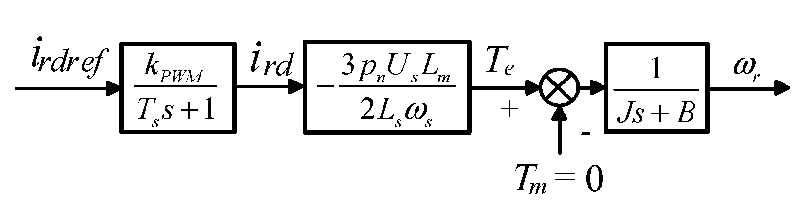
4.1.1. Start-Up in Generating Mode

During start-up of generating mode, since the unit has not been connected to the grid, the output power of the unit to the grid is 0. The specific model is equivalent to the relationship shown in Formula (15), and the duration is the time when the unit speed is loaded to the rated speed:

$$P_{S1}=0, 0\le t<{\tau }_1,$$

(15)

where P_s1 is the output power of the DFVSPS unit to the grid during the start-up, and τ₁ is the duration of the start-up. The calculation of τ₁ is as follows.

The control diagram of the whole unit in this stage is shown in Figure 15.

The guide vane opening of pump turbine is set at 6% in the start-up stage and maintains the entire start-up process. Therefore, the dynamic process of the pump turbine is neglected, and P_m = 6% (This value is expressed as per unit value, which needs to be converted to an actual value when connected with DFIM), and the start-up process can be simplified to the Equation (16):

$$\{\begin{array}{l}J\frac{d{\omega }_m}{dt}=\frac{P_m}{{\omega }_m}-B_m{\omega }_m\hfill \\ P_m=6\%·P_{base}\hfill \end{array}.$$

(16)

It can be seen from the above equation that τ₁ depends on the mechanical parameter, friction factor of DFIM, and the no-load guide vane opening. According to the values of the relevant parameters in this paper, τ₁ = 94 s.

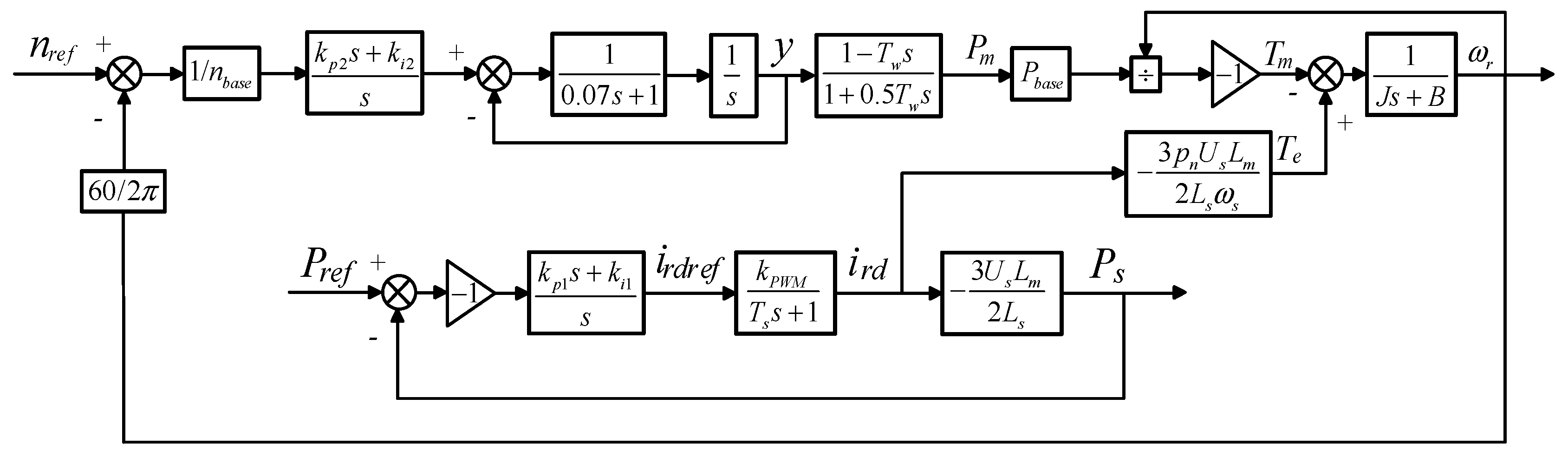
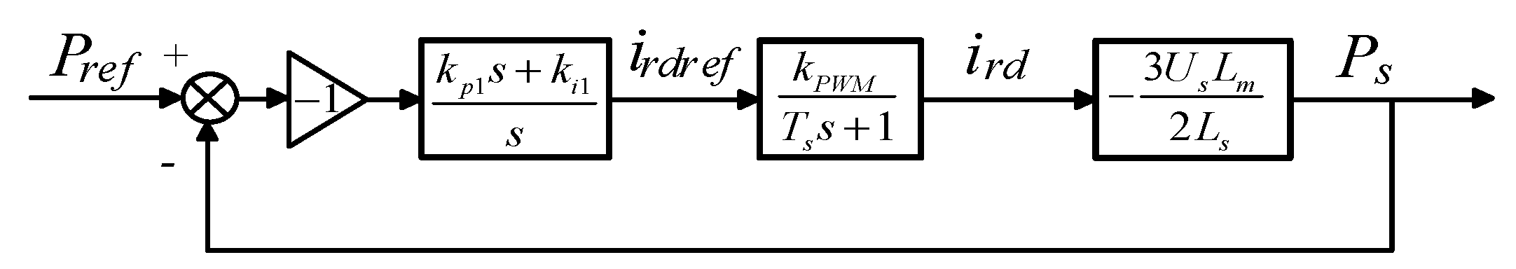
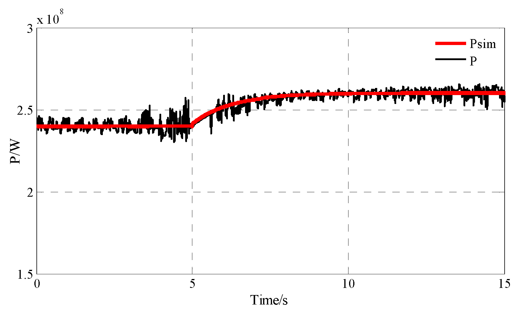
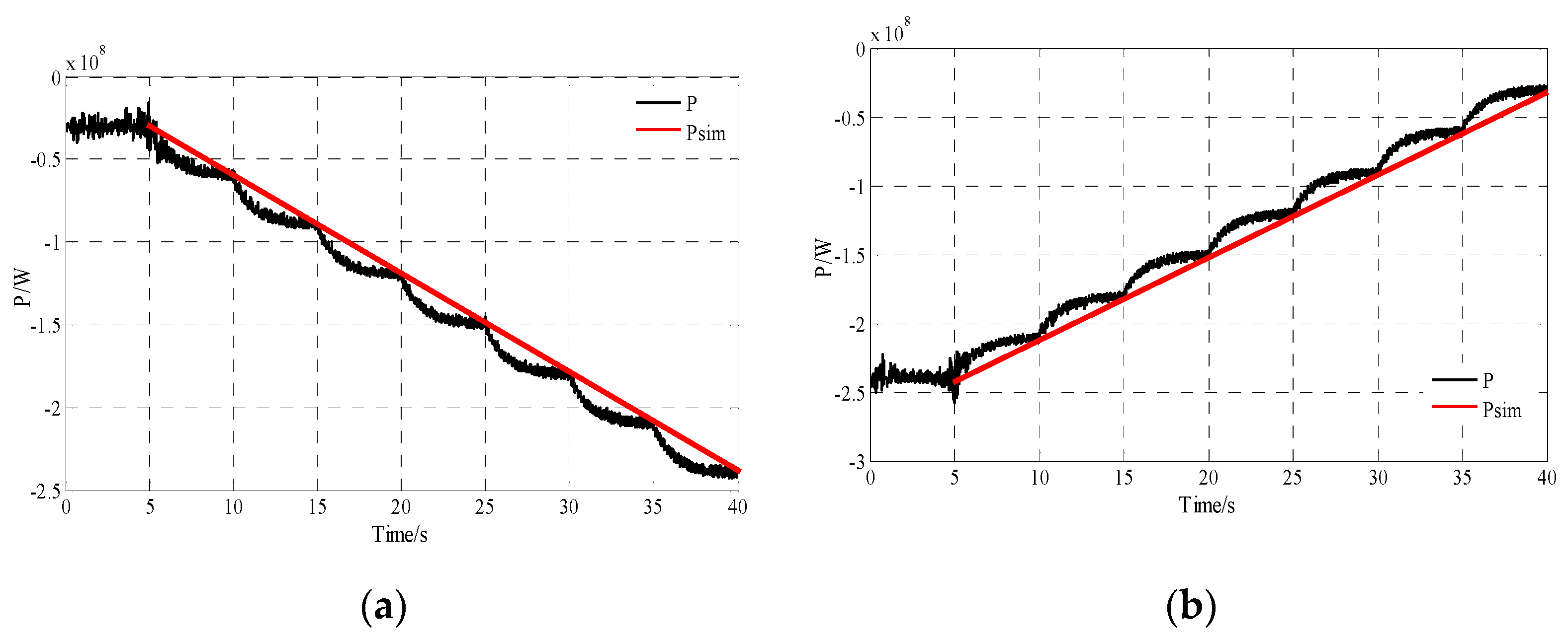
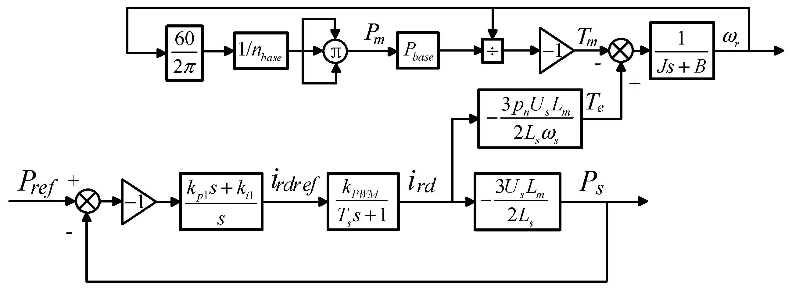
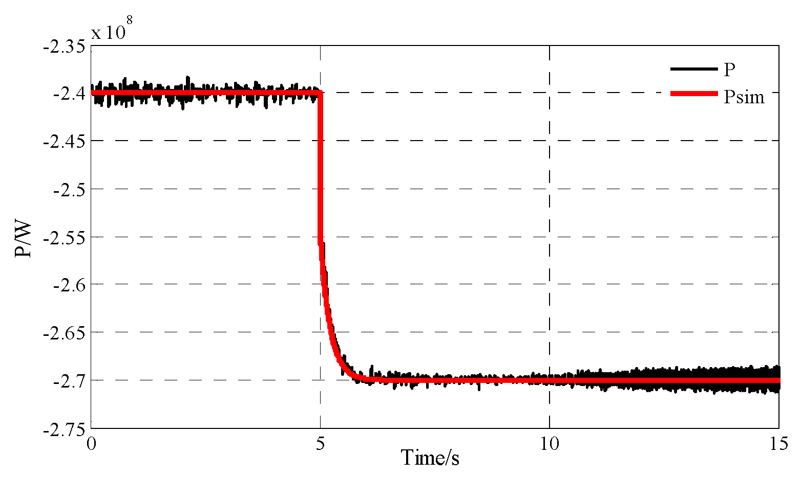
4.1.2. On-Grid Operation Stage

According to the control method of DFVSPS unit and the mathematical models of each part, the control block diagram of the power priority control strategy can be obtained as shown in Figure 16.

By observing the control block diagram, the following conclusions can be drawn:

(1)

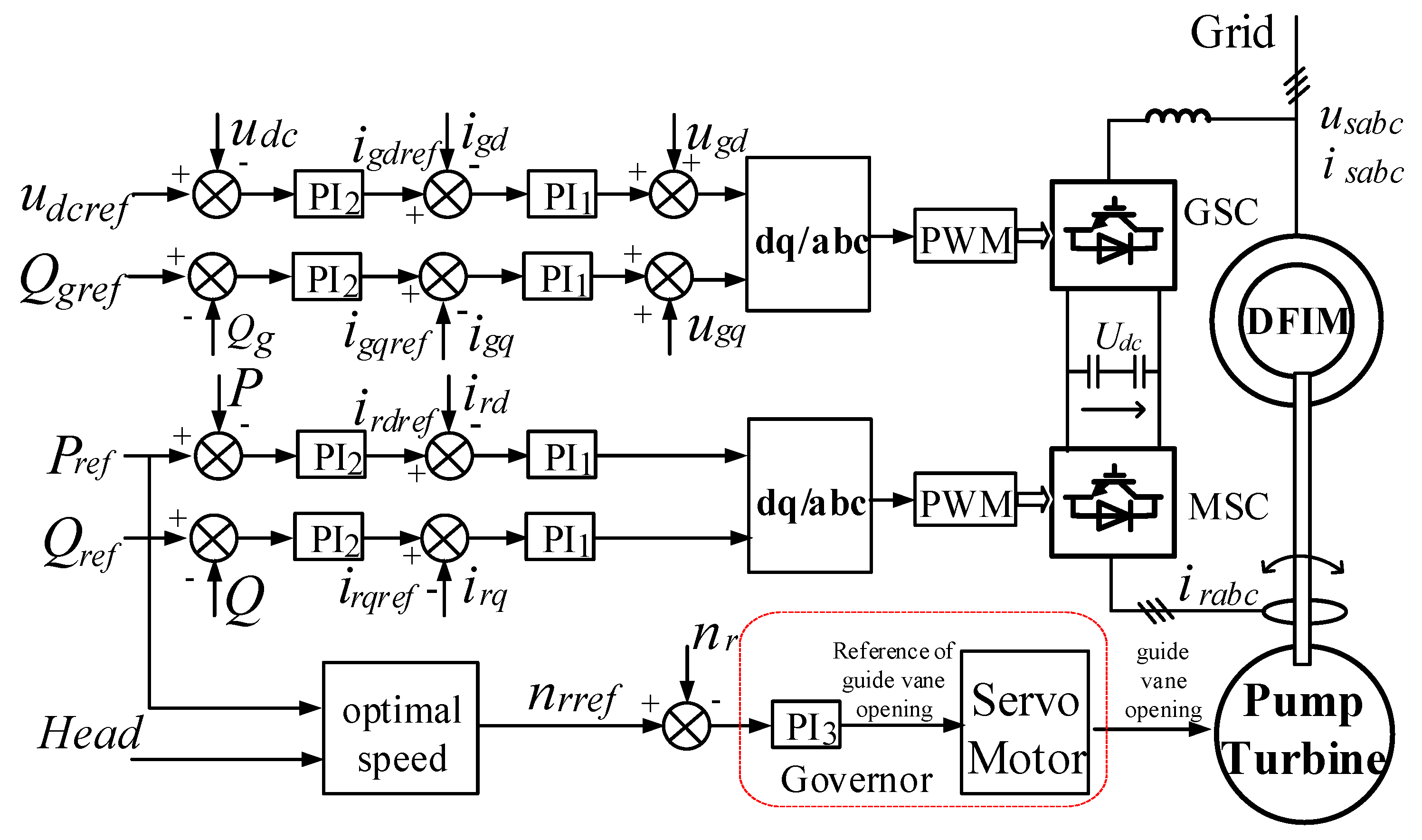
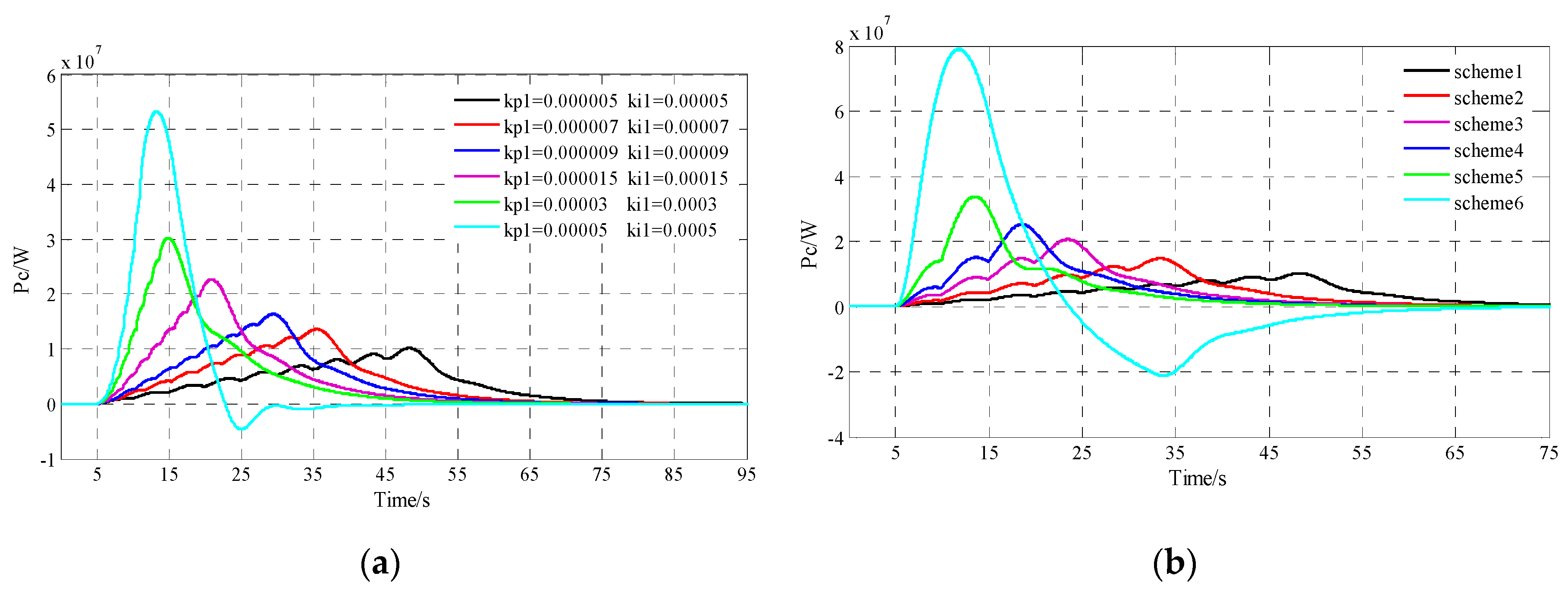
The stator side power control closed loop is an independent control loop, and its control effect is affected by the PI regulator parameters k_p1, k_i1, PWM converter switching frequency, and electromagnetic parameters of the DFIM, etc.

(2)

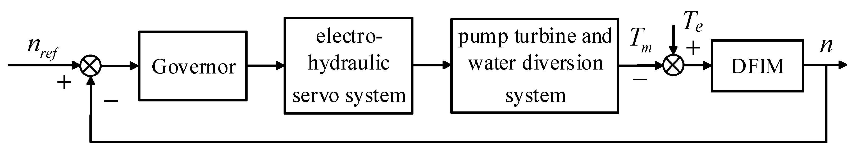
The speed control closed loop is mainly used to control the guide vane control system of pump turbine. The regulation of the speed closed loop is affected by the stator side power control closed loop, as well as by parameters such as water inertia time constant of pump turbine, pump turbine governor parameters k_p2, k_i2, and mechanical parameters of DFIM, etc.

Through the above conclusions, the adjustment of the stator side power control closed loop is not affected by the speed control closed loop. The power control closed loop is an electrical adjustment process, so it can quickly track the reference value. The response time of the speed control closed loop is longer due to the existence of the significant inertia, but since it does not affect the power control closed loop (without considering the capacity of the converter), it does not affect the speed of power regulation. Thus, the waveforms in Figure 11 and Figure 14 can be explained.

The focus of this paper is on the modelling and application of the output power of the unit. It seems to be independent from the speed control closed loop. In fact, the circulating power of the converter is the slip power, which is affected by the speed control closed loop. Due to the limitation of the converter capacity, it will affect the power adjustment range and adjustment speed; the analysis is as follows.

In the load ramping stage and the load rejection stage, the trial-and-error method is used to determine the PI parameters in the aforementioned simulation, and the power step control is adopted to increase or decrease 30 MW every 5 s. At this stage, in order to simplify the simulation model, a straight line with a certain slope is used to replace this part of the model, as shown in Equations (17) and (18):

$$p_{{}_{SG}}=p_{g0}·\frac{t-{\tau }_1}{N_{SG}}, {\tau }_1\le t<{\tau }_1+N_{SG},$$

(17)

$$p_{GS}=p_{g1}·\left(1-\frac{t-{\tau }_2}{N_{GS}}\right), {\tau }_2\le t<{\tau }_2+N_{GS},$$

(18)

where P_g0 is the power increased during the load ramping stage, P_g1 is the power reduced during the load rejection stage, τ₂ is the start time of the load rejection stage, N_SG and N_GS are the time used in the load ramping stage and load rejection stage, and Equation (17) is the load ramping stage. Equation (18) indicates the load rejection stage. The values of P_g0, P_g1, N_SG, and N_GS characterize the rate of power change during the load ramping stage and load rejection stage. The values are related to the limits of the converter capacity, stator current and rotor current. The analysis is as follows.

Firstly, the power control closed loop is analyzed. For the power model, different PI parameters will lead to different power rise time, and different segments will also affect the time of the whole load rise and fall stage. The response time can be calculated according to the power control closed loop, which is shown in Figure 17.

If k₂ = −3 U_sL_m/2 L_s, then the closed loop transfer function of the power control closed loop is shown in Equation (19):

$$G_c(s)=\frac{-k_2{k}_{PWM}(k_{p1}s+k_{i1})}{s(T_{s}s+1)-k_2{k}_{PWM}(k_{p1}s+k_{i1})}.$$

(19)

Since the switching frequency of the PWM link is very high and the switching frequency in simulation is 2 kHz, the influence of the PWM on the power control closed loop can be ignored. According to the characteristic equation of the power control closed loop, it can be calculated that, when the k_p1 and k_i1 are greater than 0, the characteristic equation does not have poles in the right half plane, and the closed loop is stable. The response of the power control closed loop to the step signal is solved as follows.

If –k₂k_p1 = m, −k₂k_i1 = n, the response of the power control closed loop to the step signal is:

$$Y(s)=\frac{1}{s}·\frac{ms+n}{(1+m)s+n}.$$

(20)

The corresponding time-domain expression is:

$$y(t)=1-\frac{1}{1+m}{e}^{\frac{-n}{1+m}t}.$$

(21)

The larger the parameters k_p1 and k_i1, the shorter the response time of the step signal, as shown in

Table 2. Response time of step signal under different PI parameters.

kp1	0.000005	0.000007	0.000009	0.000015	0.00003	0.00005
ki1	0.00005	0.00007	0.00009	0.00015	0.0003	0.0005
response time	5.0	3.5	2.8	1.8	1.1	0.75

(The PI parameters can be arbitrarily selected within the range of kp1 > 0, ki1 > 0, and different parameters correspond to different response times.).

The above table shows the response time of the power control closed loop after each stacking step instruction. For the load ramping stage and load rejection stage, in order to reduce the influence of the power adjustment on the speed, the method of segmented superimposed power command is adopted. Taking the unit parameters selected in this paper as an example, the rated power of the unit is 300 MW, and the no-load grid-connected power is 30 MW. It is necessary to superimpose a further 270 MW power from no-load power to rated power. The specific number of segments can be divided into the following types: scheme 1: each stack is 30 MW and nine times; scheme 2: each stack is 45 MW and six times; scheme 3: each stack is 67.5 MW and four times; scheme 4: each stack is 90 MW and three times; scheme 5: each stack is 135 MW and two times; scheme 6: adjust 270 MW at a time. The effect of power control closed loop with different response times and different number of segments is shown in Figure 18.

According to Figure 18a, it can be found that, when the number of segments is the same, the response time of the power control closed loop is different with different regulator parameters. The larger the parameter of the PI regulator, the shorter the response time, such as the parameter K_p1 = 0.00005, k_i1 = 0.0005, loading 270 MW power only takes about 7 s; Figure 18b is the waveform of the power control closed loop at the load ramping stage with the same response time and different number of segments. It can find that the fewer number of segments, the shorter the response time. For example, when all 270 MW power is loaded at one time, the time needed for load ramping stage is only 5 s.

During the load ramping stage and load rejection stage, different response times and number of segments are used, and the response of the speed control closed-loop is also different. Since the power flowing through the converter is the slip power, the converter power is constantly adjusted when the speed is continuously adjusted. The following two figures show the effect on converter power with different response times and different number of segments.

Figure 19a shows that, when the number of segments is the same, the fluctuation of converter power with different regulator parameters used in the power control closed-loop. It can be found that the larger the parameter of the PI regulator, the shorter the response time, but it will cause greater fluctuation on speed, and also greater power flowing through the converter. For example, under the parameters k_p1 = 0.00005, k_i1 = 0.0005, it takes only about 7 s to upload 270 MW, but the forward power of the converter is 54 MW, the reverse power is about 4 MW, so the capacity of the converter needs to be 58 MW; Figure 19b shows the fluctuation of converter power when the response time is the same, but the number of segments is different. The fewer the number of segments, the shorter the response time of load ramping stage will be, and also the converter power will greatly increase. For example, when uploading all 270 MW power at a time, the time required for the load ramping stage is only 5 s, but the forward power of the converter is about 80 MW, the reverse power is about 20 MW, and the capacity of the converter needs to be 100 MW.

Figure 19 shows the power change of the converter only considering the load ramping stage. Considering the load rejection stage and the pump mode, the converter power flow direction will be opposite to that of the load ramping stage, so the capacity requirement of converter is higher.

For the equivalent of the power model in the load ramping stage and load rejection stage, the parameters of P_g0, P_g1, N_SG, and N_GS can be selected according to the parameters of the power control closed loop and the related limits of the rotor side voltage, current, capacity of converter and other parameters. The overall conclusion is the higher the power change and the shorter the response time, the higher the corresponding converter capacity. Therefore, the parameters of the load ramping stage and load rejection stage can be selected in terms of achievability, economy, and the like.

The parameter selected in the simulation is: k_p1 = 0.000005, k_i1 = 0.00005, so the response time of each segment is 5 s, each segment is superimposed 30 MW, superimposed seven times to reach 240 MW. This choice requires small capacity, easy implementation, and high economy. According to the selected parameters, P_g0 = 210 MW, P_g1 = 210 MW, N_SG = 35 s, N_GS = 35 s, the comparison of the waveforms before and after the equivalent of the load ramping stage and load rejection stage is shown in Figure 20. The red line in the figure is unit active power of simplified model obtained by Equations (17) and (18). In addition, the black line is the unit active power simulation waveform obtained by the electromagnetic transient simulation model.

When the unit is operating near the stable operation point, the power regulation is still completed by the power control closed loop but unlike the wide range of power changes that occur during the load ramping stage and load rejection stage. Therefore, it can be expressed by the transfer function of power control closed loop, as shown in the following equation:

$$p_G=G_1\left(s\right)P_{ref}, {\tau }_1+N_{SG}\le t<{\tau }_2,$$

(22)

where G₁(s) is the transfer function of power control closed loop, shown in Formula (19).

The equivalent effect of the stable operation stage is shown in Figure 21. The red line in the figure is unit active power of simplified model obtained by Equation (22) and the black line is the unit active power simulation waveform obtained by the electromagnetic transient simulation model.

τ₂ is the end time of the stable operation stage. In the simulation of this paper, after the power increases by 20 MW in this stage, it needs to be reduced by 20 MW and returned to 240 MW, in order to facilitate the load rejection stage. Thus, the simulation time of the whole stable operation stage is twice that of the load increase, and each segment contains the time for the speed to stabilize after the power adjustment. The time for each segment is 40 s, and the duration of the stable operation stage is 80 s.

4.1.3. Orderly Shutdown Stage

In the shutdown stage of pump mode, after the unit is disconnected from the grid, the output power to the grid is also reduced to zero. The power at this stage can be expressed by Equation (23):

$$P_{S2}=0, {\tau }_2+N_{GS}\le t<{\tau }_3,$$

(23)

where τ₃ is the end time of shutdown stage, and the duration of this stage can be calculated by Formula (24):

$$\{\begin{array}{l}J\frac{d{\omega }_m}{dt}=T_{\mathrm{e}}-B_m{\omega }_m\hfill \\ T_e=-\frac{3p_n{U}_s{L}_m}{2L_s{\omega }_s}{i}_{dr}\hfill \end{array}.$$

(24)

At this time, the stator side of the DFIM is short-circuited by a small resistor. Therefore, the value of the voltage U_s is different from that of the on-grid operation stage. The electromagnetic torque opposite to the rotation direction can be generated by applying the corresponding command current to the d-axis of rotor side converter to accelerate the shutdown process of the unit. Referring to the parameters selected in the simulation of this paper, the duration of the shutdown stage is 60.4 s.

4.2. Pump Mode

4.2.1. Start-up in Pump Mode

During start-up of pump mode, since the unit has not been connected to the grid, the output power of the unit to the grid is 0. The specific model is equivalent to the relationship shown in Formula (25), and the duration is the time when the unit speed is loaded to the rated speed:

$$P_{S3}=0, 0\le t<{\tau }_1,$$

(25)

where P_s3 is the output power of the DFVSPS unit to the grid during the start-up, and τ₁ is the duration of the start-up. The calculation of τ₁ is as follows.

The control diagram of the whole unit in this stage is shown in Figure 22.

During the start-up process, the stator side of DFIM is short-circuited through a small resistor. Therefore, the stator-side voltage is different from that of the on-grid operation stage. By controlling the d-axis current of the rotor-side converter, the corresponding electromagnetic torque can be generated to start the unit. Simplified to Equation (26),

$$\{\begin{array}{l}J\frac{d{\omega }_m}{dt}=T_e-B_m{\omega }_m\hfill \\ T_e=-\frac{3p_n{U}_s{L}_m}{2L_s{\omega }_s}\frac{k_{PWM}}{T_{s}s+1}{i}_{rdref}\hfill \end{array}.$$

(26)

It can be seen from the above equation that τ₁ depends on the mechanical parameter, friction factor of DFIM, and the d-axis current. According to the values of the relevant parameters in this paper, τ₁ = 60 s.

4.2.2. On-Grid Operation Stage

In the previous section, the control methods of generating mode and pump mode are researched. The pump turbine model are different under the two working modes, and the control strategies are the same. Therefore, when the model is simplified under pump mode, the analysis method is consistent with that of the generating mode. Only a few differences are analyzed below.

During the load ramping stage and load rejection stage, the pump turbine operates at the small guide vane opening, so the control process is exactly the same as the generating mode, except that the same guide vane opening corresponds to different mechanical power. Since the converter flows through the slip power, the working mode does not affect the power of the converter, and the power flow direction is opposite to that in the generating mode. The conclusion is that the more power is regulated and the shorter the response time, the larger the capacity the converter required. The equivalent method of the load ramping stage and load rejection stage are consistent with generating mode. In addition, it can be expressed by the following formula:

$$p_{{}_{SP}}=p_{P0}·\frac{t-{\tau }_1}{N_{SP}}, {\tau }_1\le t<{\tau }_1+N_{SP},$$

(27)

$$p_{PS}=p_{P1}·\left(1-\frac{t-{\tau }_2}{N_{PS}}\right), {\tau }_2\le t<{\tau }_2+N_{PS},$$

(28)

where P_p0 is the power increased during the load ramping stage, P_p1 is the power reduced during the load rejection stage, τ₂ is the start time of the load rejection stage, N_SP and N_PS are the time used in the load ramping stage and load rejection stage, and Equation (27) is the load ramping stage. Equation (28) indicates the load rejection stage.

The parameter selected in the simulation is: k_p1 = 0.000005, k_i1 = 0.00005, so the response time of each segment is 5 s, and each segment is superimposed 30 MW, superimposed seven times to reach 240 MW. This choice requires small capacity, easy implementation, and high economy. According to the selected parameters, P_p0 = 210 MW, P_p1 = 210 MW, N_SP = 35 s, N_PS = 35 s, the comparison of the waveforms before and after the equivalent of the load ramping stage and load rejection stage is shown in Figure 23. The red line in the figure is unit active power of simplified model obtained by Equations (27) and (28). In addition, the black line is the unit active power simulation waveform obtained by the electromagnetic transient simulation model.

Stable operation stage: When the DFVSPS runs at stable operation stage under pump mode, the pump turbine is located in the part of large guide vane opening, and the input power of the pump turbine is proportional to the cube of the unit speed. The control block diagram of this stage is shown in Figure 24.

Compared with the generating mode, the power control closed loop is the same. The difference mainly exists with the speed control closed loop. Since this part only models the output power of DFVSPS unit, the equivalent formula similar with Formula (22), as shown in Equation (29). According to the parameters of the pump mode, k_p2 = 0.00005, k_i2 = 0.0005. Bring the parameter to Formula (29), the equivalent effect is shown in Figure 25. The red line in the figure is unit active power of a simplified model obtained by Equation (29) and the black line is the unit active power simulation waveform obtained by the electromagnetic transient simulation model:

$$p_P=G_1\left(s\right)P_{ref}, {\tau }_1+N_{SP}\le t<{\tau }_2.$$

(29)

τ₂ is the end time of the stable operation stage. In the simulation of this paper, after the power increases by 30 MW in this stage, it needs to be reduced by 30 MW and returned to 240 MW, in order to facilitate the load rejection stage. Thus, the simulation time of the whole stable operation stage is twice that of the load increase, and each segment contains the time for the speed to stabilize after the power adjustment. The time for each segment is 40 s, and the duration of the stable operation stage is 80 s.

4.2.3. Orderly Shutdown Stage

The method used in the shutdown of the pump mode is the same as that in the generating mode. The method of electromagnetic braking is adopted. The output power of the unit is also 0 at this stage. The equivalent expression is shown in Formula (30):

$$P_{S4}=0, {\tau }_2+N_{PS}\le t<{\tau }_3,$$

(30)

where P_s4 is the power during the shutdown stage, τ₃ is the end time of shutdown stage. The duration calculation method at this stage is consistent with the generating mode. According to the data selected in this paper, the duration of this stage is 50 s.

4.3. Comparison of Simulation Time

Simulation time of each stage before model simplification is shown in

Table 3. Simulation time of each stage before model simplification.

	Generating Mode	Pump Mode
Start-up	2 min	2 min
Load ramping stage	2 h and 58 min	2 h and 40 min
Stable operation stage	3 h and 4 min	2 h and 22 min
Load rejection stage	2 h and 50 min	2 h and 55 min
Shutdown stage	10 min	10 min

.

The power output model of each stage in the switching process of DFVSPS unit has been obtained above. Considering the no-load running time after grid connection and before the disconnection, the power model of the whole transition process is shown in Figure 26 and Figure 27. This simulation model only needs about 20 s to simulate the entire switching process.

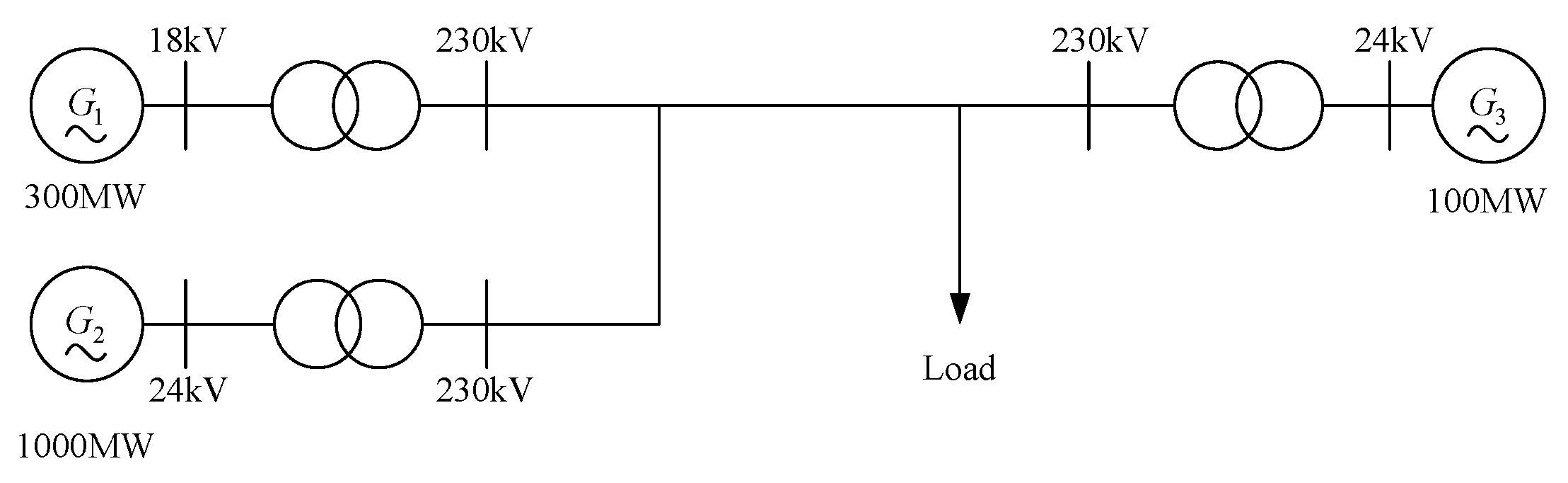
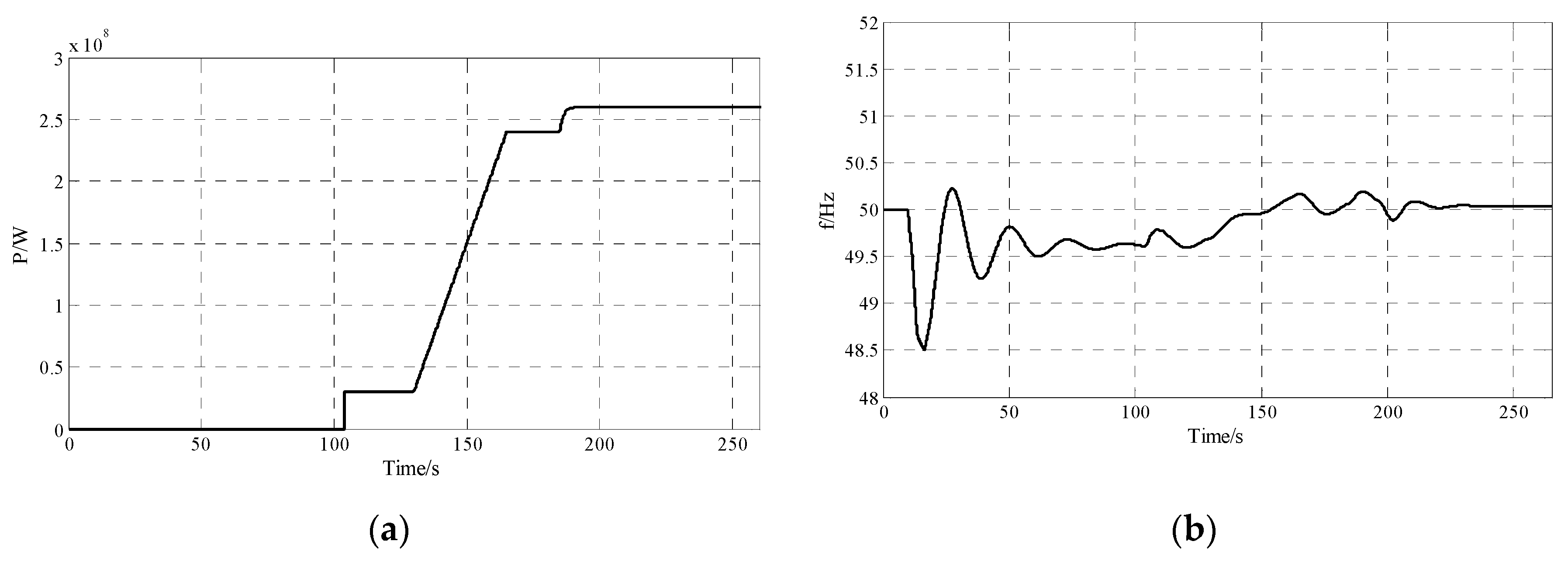
5. Example of Power System Simulation Using the Simplified Model

A system example is given, including a 300 MW DFVSPS unit G₁, a 1000 MW thermal power unit G₂, a 100 MW hydroelectric unit G₃ and a load, as shown in Figure 28.

The output power model established in this paper is applied to the G₁ in the diagram.

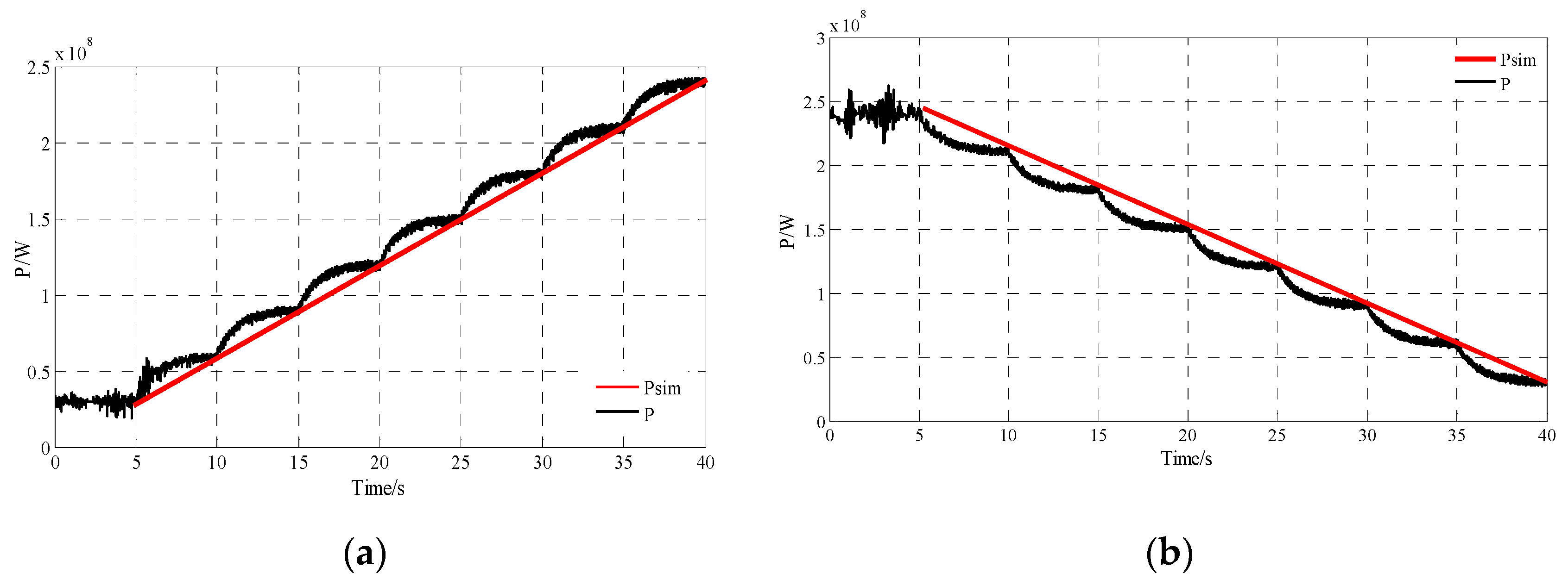
5.1. Generating Mode

In the initial state, the output power of each generator is P_G2 = 500 MW, P_G3 = 86 MW, load P_L = 586 MW, and the frequency of system is 50 Hz. At t = 10 s, the load increases by 260 MW, and there will be a power shortage, which will cause instability of the system. Thus, the G1 needs to be run on generating mode to provide this power. The simulation results are shown in Figure 29.

At t = 10 s, G1 is started, and t = 10 s to t = 104 s is the start-up stage, t = 104 s to t = 130 s is the no load operation stage, t = 130 s to t = 165 s is the load increasing stage, and t = 165 s to t = 265 s is the stable operation stage. The power flow of the 18-kV bus is shown in Figure 29a, which starts to increase at t = 104 s, reaching 240 MW at t = 165 s and reaching 260 MW at t = 190 s. The frequency of system is shown in Figure 29b. When the load suddenly increases, the system frequency deviates from the rated value. After the DFVSPS connected to the grid, the frequency returns to a reasonable value.

5.2. Pump Mode

In the initial state, the output power of each generator is P_G2 = 565 MW, P_G3 = 86 MW, load P_L = 651 MW, and the frequency of system is 50 Hz. At t = 10 s, the load decreases by 270 MW, and there will be a power surplus, which will cause instability of the system. Thus, the G1 needs to be run on pump mode to absorb this power. The simulation results are shown in Figure 30.

At t = 10 s, G₁ is started, and t = 10 s to t = 70 s is the start-up stage, t = 70 s to t = 90 s is the no load operation stage, t = 90 s to t = 125 s is the load increasing stage, and t = 125 s to t = 225 s is the stable operation stage. The power flow of the 18-kV bus is shown in Figure 30a, which starts to increase at t = 70 s, reaching 240 MW at t = 125 s and reaching 270 MW at t = 150 s. The frequency of system is shown in Figure 30b. When the load suddenly decreases, the system frequency deviates from the rated value. After the DFVSPS connected to the grid, the frequency returns to a reasonable value.

6. Conclusions

Based on the structure diagram of the DFVSPS unit and the mathematical models of each part, the switching process of the DFVSPS unit under generating mode and the pump mode were simulated. The power output model of each stage of DFVSPS unit was simplified in order to make the DFVSPS unit able to be applied to power system simulation, the simplified model was applied to the power system simulation, and the following conclusions are drawn.

After the power priority control strategy is adopted for the DFVSPS unit, and the electromagnetic torque and the mechanical torque of DFIM are respectively controlled by the power control closed loop and the speed control closed loop, so two closed loops are coupled together through the rotating shaft. The power control closed loop is an independent control closed loop, and the speed control closed loop is adjusted by speed, so the control characteristic of the speed control closed loop is affected by the power control closed loop.

The electromagnetic transient simulation includes the change of all parameters in the whole switching process of DFVSPS unit. Due to the switching frequency of the converter, the simulation step is very short, so the simulation speed is slow and the data volume is large, which is not suitable for studying the influence of switching process of DFVSPS unit on the power system. The simplified model can well characterize the power output characteristics of the DFVSPS unit, greatly shortened the simulation time, and it can replace the electromagnetic transient model for power system simulation.

The DFVSPS unit has a good compensation ability for the power fluctuation of a power system.

For the compensation speed and compensation range for the power fluctuation of DFVSPS unit, after analysis, it is found that the larger the compensation range, the faster the compensation speed, and the higher the requirements for converter capacity and DFIM stator and rotor voltage and current levels. Therefore, the compensation range and compensation speed are constrained by parameters such as converter capacity.

References

1. Saiju, R.; Koutnik, J.; Krueger, K. Dynamic analysis of start-up strategies of AC excited Double Fed Induction Machine for pumped storage power plant. In Proceedings of the 2009 13th European Conference on Power Electronics and Applications, Barcelona, Spain, 8–10 September 2009; pp. 1–8. [Google Scholar]
2. O’Dwyer, C.; Flynn, D. Using Energy Storage to Manage High Net Load Variability at Sub-Hourly Time-Scales. IEEE Trans. Power Syst. 2015, 30, 2139–2148. [Google Scholar] [CrossRef]
3. Castillo, A.; Gayme, D.F. Grid-scale energy storage applications in renewable energy integration: A survey. Energy Convers. Manag. 2014, 87, 885–894. [Google Scholar] [CrossRef]
4. Pérez-Díaz, J.I.; Chazarra, M.; García-González, J.; Cavazzini, G.; Stoppato, A. Trends and challenges in the operation of pumped-storage hydropower plants. Renew. Sustain. Energy Rev. 2015, 44, 767–784. [Google Scholar] [CrossRef]
5. Vargas-Serrano, A.; Hamann, A.; Hedtke, S.; Franck, C.M.; Hug, G. Economic benefit analysis of retrofitting a fixed-speed pumped storage hydropower plant with an adjustable-speed machine. In Proceedings of the 2017 IEEE Manchester PowerTech, Manchester, UK, 18–22 June 2017. [Google Scholar]
6. Sivakumar, N.; Das, D.; Padhy, N.P. Variable speed operation of reversible pump-turbines at Kadamparai pumped storage plant–A case study. Energy Convers. Manag. 2014, 78, 96–104. [Google Scholar] [CrossRef]
7. Li, D.; Wang, H.; Li, Z.; Nielsen, T.K.; Goyal, R.; Wei, X.; Qin, D. Transient characteristics during the closure of guide vanes in a pump-turbine in pump mode. Renew. Energy 2018, 118, 973–983. [Google Scholar] [CrossRef]
8. Sun, H.; Xiao, R.; Liu, W.; Wang, F. Analysis of S Characteristics and Pressure Pulsations in a Pump-Turbine with Misaligned Guide Vanes. J. Fluids Eng. 2013, 135, 511011. [Google Scholar] [CrossRef] [PubMed]
9. Xiao, Y.X.; Zhu, W.; Wang, Z.; Zhang, J.; Zeng, C.; Yao, Y. Analysis of the internal flow behavior on S-shaped region of a Francis pump turbine on turbine mode. Eng. Comput. 2016, 33, 543–561. [Google Scholar] [CrossRef]
10. Liu, J.; Liu, S.; Sun, Y. Three-dimensional flow simulation of transient power interruption process of a prototype pump-turbine at pump mode. J. Mech. Sci. Technol. 2013, 27, 1305–1312. [Google Scholar] [CrossRef]
11. Fu, X.; Li, D.; Wang, H.; Zhang, G.; Li, Z.; Wei, X. Analysis of transient flow in a pump-turbine during the load rejection process. J. Mech. Sci. Technol. 2018, 32, 2069–2078. [Google Scholar] [CrossRef]
12. Khodayar, M.E.; Abreu, L.; Shahidehpour, M. Transmission-constrained intrahour coordination of wind and pumped-storage hydro units. IET Gener. Transm. Distrib. 2013, 7, 755–765. [Google Scholar] [CrossRef]
13. Ma, T.; Yang, H.; Lu, L.; Peng, J. An Optimization Sizing Model for Solar Photovoltaic Power Generation System with Pumped Storage. Energy Procedia 2014, 61, 5–8. [Google Scholar] [CrossRef] [Green Version]
14. Schmidt, J.; Kemmetmüller, W.; Kugi, A. Modeling and static optimization of a variable speed pumped storage power plant. Renew. Energy 2017, 111, 38–51. [Google Scholar] [CrossRef]
15. Joseph, A.; Desingu, K.; Semwal, R.R.; Chelliah, T.R.; Khare, D. Dynamic Performance of Pumping Mode of 250 MW Variable Speed Hydro-Generating Unit Subjected to Power and Control Circuit Faults. IEEE Trans. Energy Convers. 2017, 33, 430–441. [Google Scholar] [CrossRef]
16. Joseph, A.; Chelliah, T.R. A Review of Power Electronic Converters for Variable Speed Pumped Storage Plants: Configurations, Operational Challenges and Future Scopes. IEEE J. Emerg. Sel. Top. Power Electr. 2017, 6, 103–119. [Google Scholar] [CrossRef]
17. Zuo, Z.; Fan, H.; Liu, S.; Wu, Y. S-shaped characteristics on the performance curves of pump-turbines in turbine mode–A review. Renew. Sustain. Energy Rev. 2016, 60, 836–851. [Google Scholar] [CrossRef]
18. Feltes, J.; Koritarov, V.; Guzowski, L.; Donalek, P.; Grande-Moran, C.; Troullie, C.; Koritarov, V. Modeling Adjustable Speed Pumped Storage Hydro Units Employing Doubly-Fed Induction Machines; Argonne National Lab. (ANL): Argonne, IL, USA, 2013. [Google Scholar]
19. Demello, F.P.; Koessler, R.J.; Agee, J.; Anderson, P.M.; Doudna, J.H.; Fish, J.H.; Hamm, P.A.L.; Kundur, P.; Lee, D.C.; Rogers, G.J.; et al. Hydraulic turbine and turbine control models for system dynamic studies. IEEE Trans. Power Syst. 1992, 7, 167–179. [Google Scholar]
20. Zuo, Z.; Liu, S. Flow-induced instabilities in pump-turbines in China. Engineering 2017, 3, 504–511. [Google Scholar] [CrossRef]
21. Li, D.; Zuo, Z.; Wang, H.; Liu, S.; Wei, X.; Qin, D. Review of positive slopes on pump performance characteristics of pump-turbines. Renew. Sustain. Energy Rev. 2019, 112, 901–916. [Google Scholar] [CrossRef]
22. Liang, J.; Harley, R.G. Pumped storage hydro-plant models for system transient and long-term dynamic studies. Power Energy Soc. Gen. Meet. IEEE 2010, 89, 1–8. [Google Scholar]
23. Golkhandan, R.K.; Aghaebrahimi, M.R.; Farshad, M. Control strategies for enhancing frequency stability by DFIGs in a power system with high percentage of wind power penetration. Appl. Sci. 2017, 7, 1140. [Google Scholar] [CrossRef]
24. Li, B.; Liu, J.; Wang, X.; Zhao, L. Fault Studies and Distance Protection of Transmission Lines Connected to DFIG-Based Wind Farms. Appl. Sci. 2018, 8, 562. [Google Scholar] [CrossRef]
25. Cai, G.; Chen, X.; Sun, Z.; Yang, D.; Liu, C.; Li, H. A Coordinated Dual-Channel Wide Area Damping Control Strategy for a Doubly-Fed Induction Generator Used for Suppressing Inter-Area Oscillation. Appl. Sci. 2019, 9, 2353. [Google Scholar] [CrossRef]
26. Zeng, W.; Yang, J.; Hu, J. Pumped storage system model and experimental investigations on S-induced issues during transients. Mech. Syst. Signal Process. 2017, 90, 350–364. [Google Scholar] [CrossRef]
27. Shen, Y.; Ji, Z.; Pan, T.; Wu, D. A no-load grid-connected strategy based on one-cycle control for doubly-fed wind power system. In Proceedings of the 2014 IEEE Energy Conversion Congress and Exposition (ECCE), Pittsburgh, PA, USA, 14–18 September 2014; pp. 1822–1826. [Google Scholar]
28. Kuwabara, T.; Shibuya, A.; Furuta, H.; Furuta, H.; Kita, E.; Mitsuhashi, K. Design and dynamic response characteristics of 400 MW adjustable speed pumped storage unit for Ohkawachi power station. IEEE Trans. Energy Convers. 1996, 11, 376–384. [Google Scholar] [CrossRef]
29. Lung, J.K.; Lu, Y.; Hung, W.L.; Kao, W. Modeling and dynamic simulations of doubly fed adjustable-speed pumped storage units. IEEE Trans. Energy Convers. 2007, 22, 250–258. [Google Scholar] [CrossRef]
30. Laabidi, M.; Rebhi, B.; Kourda, F.; Elleuch, M.; Ghodbani, L. Braking of induction motor with the technique of discrete frequency control. In Proceedings of the 2010 7th International Multi- Conference on Systems, Signals and Devices, Amman, Jordan, 27–30 June 2010; pp. 1–6. [Google Scholar]
Figure 1. Structure diagram of the DFVSPS.
Applsci 09 03368 g001
Figure 2. Schematic diagram of pump turbine regulating system.
Applsci 09 03368 g002
Figure 3. ac servo motor/ electro-hydraulic actuator type servo system.
Applsci 09 03368 g003
Figure 4. Full-characteristic curve of pump-turbine and main transition process path.
Applsci 09 03368 g004
Figure 5. Comparison of operating characteristic curves between conventional turbine and pump turbine.
Applsci 09 03368 g005
Figure 6. Simplified nonlinear turbine model.
Applsci 09 03368 g006
Figure 7. Pump mode model under small guide vane opening.
Applsci 09 03368 g007
Figure 8. Waveforms of start-up in generating mode. (a) guide vane opening; (b) mechanical power; (c) speed.
Applsci 09 03368 g008
Figure 9. Comparison of three-phase voltage before and after grid connection.
Applsci 09 03368 g009
Figure 10. Overall control diagram of power priority control strategy.
Applsci 09 03368 g010
Figure 11. Simulation waveforms of unit in generating mode: (a) active power in load ramping stage; (b) active power in stable operation stage; (c) active power in load rejection stage; (d) speed in stable operation stage; (e) guide vane opening in stable operation stage; (f) actual dynamic responses for a DFVSPS unit in stable operation.
Applsci 09 03368 g011
Figure 12. Waveform of shutdown stage in generating mode. (a) Tm and Te; (b) speed.
Applsci 09 03368 g012
Figure 13. Speed waveform during start-up stage.
Applsci 09 03368 g013
Figure 14. Simulation waveforms of unit in pump mode: (a) active power in load ramping stage; (b) active power in stable operation stage; (c) active power in load rejection stage; (d) speed in stable operation stage; (e) guide vane opening in stable operation stage; (f) actual dynamic responses for a DFVSPS unit in stable operation.
Applsci 09 03368 g014
Figure 15. Control diagram of start-up in generating mode.
Applsci 09 03368 g015
Figure 16. Control block diagram of the power priority control strategy in generating mode.
Applsci 09 03368 g016
Figure 17. Power control closed loop.
Applsci 09 03368 g017
Figure 18. Effect of power control closed loop. (a) different response times; (b) different number of segments.
Applsci 09 03368 g018
Figure 19. Change diagram of converter power. (a) different response times; (b) different number of segments.
Applsci 09 03368 g019
Figure 20. Comparison of active power waveform before and after equivalent. (a) load ramping stage; (b) load rejection stage.
Applsci 09 03368 g020
Figure 21. Comparison of active power waveform before and after equivalent during stable operation stage.
Applsci 09 03368 g021
Figure 22. Control diagram of start up in pump mode.
Applsci 09 03368 g022
Figure 23. Comparison of active power waveform before and after equivalent. (a) load ramping stage; (b) load rejection stage.
Applsci 09 03368 g023
Figure 24. Control block diagram of stable operation stage under pump mode.
Applsci 09 03368 g024
Figure 25. Comparison of active power waveform before and after equivalent during stable operation stage.
Applsci 09 03368 g025
Figure 26. Generating mode.
Applsci 09 03368 g026
Figure 27. Pump mode.
Applsci 09 03368 g027
Figure 28. Structure of the system example.
Applsci 09 03368 g028
Figure 29. Simulation waveform in generating mode. (a) power flow on 18-kV bus; (b) the frequency of the system.
Applsci 09 03368 g029
Figure 30. Simulation waveform in pump mode. (a) power flow on 18-kV bus; (b) the frequency of system.
Applsci 09 03368 g030