Cooperative Threads with Effective-Address in Simulated Annealing Algorithm to Job Shop Scheduling Problems

Featured Application

This research allows improving the schedule of jobs in manufacturing workshops and this increases the amount of products without having the need to increase the production machines.

Abstract

This paper presents a parallel algorithm applied to the job shop scheduling problem (JSSP). The algorithm generates a set of threads, which work in parallel. Each generated thread, executes a procedure of simulated annealing which obtains one solution for the problem. Each solution is directed towards the best solution found by the system at the present, through a procedure called effective-address. The cooperative algorithm evaluates the makespan for various benchmarks of different sizes, small, medium, and large. A statistical analysis of the results of the algorithm is presented and a comparison of performance with other (sequential, parallel, and distributed processing) algorithms that are found in the literature is presented. The obtained results show that the cooperation of threads carried out by means of effective-address procedure permits to simulated annealing to work with increased efficacy and efficiency for problems of JSSP.

1. Introduction

The job shop scheduling problem (JSSP) appears in the manufacturing industry and is classified by the theory of complexity as one of the most difficult problems to solve within the class of NP-complete problems [1], where NP, indicates non-polynomial behavior problems, that is, problems that do not have an exact algorithm that can solve them in polynomial time. Due to the difficulty of solving this problem, it is important to look for new alternatives in the solution thread in order to improve the cost/performance of the existing algorithms that attempt this type of problem for the purpose of obtaining better solutions.

In the solution of JSSP, very little information exists with regard to algorithms that apply parallel threading as a form of cooperation in order to accelerate the search for better solutions. In [2], with their branch and bound algorithm, they generate a search tree through the cooperation of 16 threads, where each thread is executed by a CPU (central processing unit). In [3], the researchers investigate the performance with multi-threading using mixed integer programming and parameter tuning with CPLEX to JSSP of 15 × 15, where CPLEX is a Simplex algorithm written in language C (C-Simplex resulted in CPLEX). In [4] with their branch and bound algorithm, the researchers propose a GPU-based parallelization in which a two level scheme is used, therefore, at each iteration, several search tree nodes are evaluated on the GPU using several thread-blocks to the blocking job shop scheduling problem. In [5], the researchers present a parallel branch and bound which is based on implicit enumeration and parallel particle swarm optimization (PSO). In parallel PSO, the model used is the master-slave model; each client evaluates its own population at the same time. The master is responsible for defining the parameters that are necessary for the population in each slave. In each iteration, each slave sends its best particle back to the master. The master sends the best received particles to all the slaves to inform them of the best particle in the group. Then each slave updates its best particle. The parallel branch and bound use the logical ring topology. It involves a simulated annealing algorithm to improve the upper bound when a timeout controller is used. The results presented for the parallel branch and bound are for small problems of up to 6 jobs and 15 machines. They only perform comparative tests of efficiency between the proposed sequential and parallel branch and bound. The results presented for the PSO are not good, and are only for medium sized problems. In [6], the researchers use a system of distributed computation compound for 12 personal computers to execute an algorithm of simulated annealing (SA) and their results are not good. In [7], the researchers report a parallel version of the simulated annealing algorithm using a procedure for parallelizing the most difficult calculation. In this case the most difficult calculation is to obtain the critical path in the disjunctive graph model. In [8], one parallel algorithm of simulated annealing is reported, which uses a distribution system of 20 computers; this algorithm manages the concept of populations in genetic algorithms, but without using a genetics operator. Very few investigations of the application of the cooperation in algorithms for JSSP exist. In [9], a novel concept of island model with islands of different sizes is proposed to scheduling problems. The proposed multi-size approach to island model makes the effectiveness of the island-based algorithm independent from the particular population size which is identical for all islands in the canonical island model, also eliminates the need to tune the population size of identical islands to ensure high efficiency. In some genetic algorithms, cooperation is applied by means of crossover of individuals that belongs to a population. This is done within local search procedures using deterministic algorithms (critical path algorithms) in order to evaluate the neighborhood function. Satisfactory results can be obtained [10,11]. Some of the algorithms that have applied cooperation with crossover in problems of JSSP have not given good results [11,12,13], this is mainly due to the fact that the methods of crossover used, are based on improving the solution with the idea of crossed neighbors in order to get better neighbors when comparing neighbors with the neighborhoods of origin, but not with the best neighbor available in the neighborhoods. The fact of not considering the best solution available for the crossover causes, that with the passage of time, the search is not directed toward a space of good solutions. Consequently, the final solution of the algorithm with cooperation generally is not satisfactory. In [14], the researchers present a hybrid genetic algorithm (GA) with parallel implementation of simulated annealing (SA) for the JSSP. The algorithm uses a GA to generate an initial population of solutions within a server machine. Every solution in the population is then distributed to a client machine. The client machine runs an SA and sends the best obtained solution to the server machine. The server again uses the GA to improve the population. This procedure GA-SA is repeated for a number of iterations. The presented results are for medium-sized benchmarks with relative errors below 3.5%. In [15], the researchers present a hybrid parallel genetic algorithm for the JSSP. The method deals with concepts of solution backbones in order to intensify the search in promising regions. They utilize path-relinking and taboo search in crossover and mutation operators. They also use the island model to store a population on each island. If after several iterations of the GA the fitness does not improve, then the subpopulations start to merge, always maintaining the size of the initial population, until in the end there is only one population. In [16], the researchers present a hybrid parallel genetic micro algorithm. The parallel implementation considers M independent GAs running M subpopulations with independent memories, genetic operations, and function evaluation (island models) in each generation. The best individuals in each subpopulation are broadcast to the other subpopulations over a communication network. Each subpopulation consists of small populations, which communicate among themselves and share information through asynchronous message passing. Although a study is presented on the efficiency (speedup) of the parallel algorithm, it appears incomplete. The study evaluates the efficiency of the parallel algorithm for each increase in the number of threads, but the efficiency is averaged and is therefore not sufficient to evaluate the algorithm. In [17], the researchers present a parallel GA for the JSSP in which active schedules are created by the priority rules of Giffler and Thompson. The model used is the master–slave model. The GA works iteratively with distributed slave populations. It does not apply cooperation between threads and sends the best results only to the master using message passing interface (MPI). The obtained results are good, and the benchmarks are of small and medium size. The cooperation with agents in SA for JSSP dynamics has also been applied, but the results in [18], show that the time consumed in communication between agents is extensive. If the existence of several agents is considered, SA works more slowly than normal when the size of the problem of JSSP is medium or bigger. Another application with agents is an agent-based parallel approach with a genetic algorithm. For this approach, the results for benchmarks of JSSP, which are small and medium, are very poor [19]. In this study, a layered architecture was used. In the lowest layer, a multi-agent system using JADE middleware was implemented which facilitated the creation of agents and their communication using MPI. In [20], the researchers present a genetic hybrid island model algorithm for JSSP, proposing a strategy based on the self-adaptation phase that generates a better balance between diversification and intensification. Such algorithm works through pseudo-parallel on a single processor system. In [21], the researchers present an effective island model genetic algorithm for JSSP, proposing a mechanism based on natural migratory selection that improves the search and avoids premature convergence. This algorithm works through pseudo-parallel on a single processor system. In [22], the researchers present an effective genetic algorithm with a critical-path-guided crossover operator for JSSP; they use the critical path in the global search method during the crossover operator. In [23], the researchers present a hybrid simulated annealing for the job shop scheduling problem. It is based on an ant colony that generates the initial population and a simulated annealing that improves the population. The algorithm works in a parallel computer with a genetic algorithm, using a crossover genetic operator inside the cycle of temperature in simulated annealing. In [24], the researchers present a parallel artificial bee colony algorithm for JSSP with a dynamic migration strategy. It determines when a colony should communicate with its neighboring colonies. Such algorithm is carried out in various colonies in parallel. In [25], the researchers present a hybrid micro-genetic multi-population algorithm with collective communication that uses a set of elite micro-populations with computational processes and improves individuals with simulated annealing.

In this paper, cooperation is applied in order to direct the search for a solution toward a space where there are good solutions to the problem. A set of simulated annealing (SSA) is generated with restart [26], where every time that a simulated annealing (SA) ends, an effective-address procedure with the solution Si obtained from that SA and the best solution Sbest obtained by the SSA up to that moment is applied. The search will be directed toward a space where there are good solutions, making the new solution obtained by the effective-address procedure more similar to the best solution obtained by the SSA.

Section one gives a brief introduction. Section two describes the formulation of the job shop scheduling problem. Section three presents the proposed simulated annealing algorithm that applies cooperative threads (SACT) and the effective-address procedure, where a CREW model (concurrent read, exclusive write) is used in implementation [27]. Section four shows the experimental results. Finally, the conclusions drawn by the present work are explained.

2. Disjunctive Formulation of Job Shop Scheduling Problem

The disjunctive formulation has several sets: A set $J$ of n jobs, where, $J=\left\{J_1,J_2,\dots ,J_n\right\}$; a set M of m machines where $M=\left\{M_1,M_2,\dots ,M_m\right\}$; and a set O of operations where $O=\left\{1, 2, 3,\dots \right\}$. These operations form k subsets of operations for each one of the jobs $\left(J_k\subseteq O\right)$ and machines $\left(M_k\subseteq O\right)$.

Each operation i has a processing time of p_i. In a job J_k, each pair of operations i, j possesses a relationship of precedence $\left(i<j\right)$. Only one operation performed by a machine M_k, can be executed at any given point in time. Given the previously mentioned problem restrictions, the function of the starting time, s of each operation can be represented in the following manner:

The constraint in (1) indicates that the starting time of the operation j must be greater than or equal to zero; meaning only positive values are accepted. The constraint in (2) is a precedence constraint. It indicates that within one job which contains operations i and j, in order for j to begin, i must be completed. The constraints in (3) are disjunctive. These constraints ensure that two operations, i and j, which are performed by the same machine M_k are not carried out simultaneously. The constraints in (4) indicate that the time necessary to complete an operation j must be less than or equal to the makespan (C_max). The objective is to minimize the makespan, defined as the maximum time of completion of the last job, which is determined according to the starting times, and can be expressed as (5). The time units in the makespan are open, thus they can be assigned as seconds, minutes, hours, and so on, as long as these are consistent units. In this work the makespan is simply labeled as units of time.

$$\forall i\in O,s_i\ge 0$$

(1)

$$\forall \left(i,j\right)\in O\wedge \left(i\prec j\right)\in J_k \left(s_i+p_i\right)\le s_j$$

(2)

$$\forall \left(i,j\right)\in O \wedge \left(i,j\right)\in M_k \left(s_i+p_i\right)\le s_j\vee \left(s_j+p_j\right)\le s_i$$

(3)

$$\forall i\in O \left(s_i+p_i\right)\le C_{max}$$

(4)

$$min\left(f\right)=min\left[\frac{max}{i\in O}\left(s_i+p_i\right)\right]$$

(5)

Figure 1 shows the disjunctive graph model G = (A, E, O) for a JSSP of 3 × 3 (three machines and three jobs). This disjunctive graph is formed by three sets. The operations set, O, is made up of the nodes in G, numbered one to nine. The processing time appears next to each operation. The beginning and ending operations (I and * respectively) are fictitious, with processing times equal to zero. The set A is composed of conjunctive arcs, each one of these arcs unites a pair of operations that belongs to the same job J_i and each one represents a precedence constraint. The operations 1, 2, and 3 are connected by these arcs and therefore form job one (J₁). Jobs two (J₂), and three (J₃) are connected in the same way with operations (4, 5, 6) and (7, 8, 9), respectively. Each clique that belongs to E contains a subset of operations that are executed by the same machine (M_k). Operations 1, 6, and 7 are executed by M₁ and generate a clique. Machines two (M₂) and three (M₃) generate a clique, each one with operations (2, 5, 8) and (3, 4, 9), respectively. The resources capacity constraints are represented between each pair of operations in E.

3. Simulated Annealing Algorithm with Cooperative Threads (SACT)

The SACT algorithm (simulated annealing with cooperative threads) generates threads (H1, …, Hn) that are administered by the operating system Windows Vista Ultimate 64 bits and which work in parallel form. Each thread generated Hi by SACT executes and controls one simulated annealing algorithm (SA) in individual form. A core of CPU carries out the control of each thread Hi. If there are more threads than cores of CPU’s, then the threads are distributed in a balanced way among the group of cores of CPU’s that the computer contains. The cooperation among the existing threads, n, allows each thread, Hi, in which simulated annealing is carried out, to know (in any instant of important time) the best solution, S_best that has been found up to that point in time. This makes it possible that a thread Hi can use the best solution S_best to realize an effective-address procedure with the solution S_{Hi_c} that is found by executing the SA algorithm. The resulting solution of the effective-address procedure is used as an initial solution in the restart of SA within the thread Hi. Because SACT constantly needs to know and upgrade the best solution S_best. The threads have the advantage of working actively and using the same memory address space. This makes the communication among them quicker [28]. The threads are able to work simultaneously.

In SACT, the threads have continuous access to a space of shared memory that stores the best found solution for the n threads at a time t. This makes it necessary to implement a CREW model, where the access to this space of shared memory must be synchronized between the threads in order to avoid conflicts of reading/writing that could cause errors or loss of information. In order to synchronize the access to this memory, the critical section is used. This guarantees that in any given instant in time, only one thread can have access to read/write, leaving the others on a waiting list.

In the operating system Windows Vista Ultimate 64 bits, the threads are administrated like objects, which are created for calling functions to the applications programming interface (API), using the MFC library [29]. In the SACT algorithm, the functions of the MFC of Microsoft visual C++, 2017, are used for the creation of the threads in a single process.

Each thread created by SACT works by carrying out the same number of identical activities, but with different data. Knowing this, a class was created that upon generating n instances for the class, n objects are generated. Each object represents a thread [30].

SACT has the possibility of generating a parent thread, which in turn generates n offspring threads, executing them in parallel form.

The SACT algorithm applies to JSSP when the objective function is minimizing the maximum time of completion of the last job, this is known as minimizing the makespan. Algorithm 1, presents the SA algorithm that is executed for each created thread Hi by SACT.

Algorithm 1 Simulated annealing executed in each generated thread Hi by SACT.

Obtain SHi, where SHi = f (UB). Give an iteration initial iter = 0, initialize values of Cf, Co, α, f(SHi_c). While (iter < Maxiter) 3.1. iter = iter+1 3.2. C = Co 3.3. While (C < Cf). 3.3.1. While (equilibrium does not exist) 3.3.1.1. S’Hi = permutation(SHi) 3.3.1.2. If(f(S’Hi) − f(SHi) ≤ 0) SHi = S’Hi 3.3.1.3. If(f(S’Hi) − f(SHi) > 0) the state is accepted with the probability $$P_{accept}=e^{-\left(\frac{f\left({S^{\prime }}_{Hi}\right)-f\left(S_{Hi}\right)}{C}\right)}$$ 3.3.1.4. $\mathsf{\rho }=\mathrm{random}\mathrm{number}\mathrm{between}(0,1)$ 3.3.1.5. If (ρ < Paccept) SHi = S’Hi 3.3.1.6. If (f(SHi) < f(SHi_c)) SHi_c = SHi 3.3.1.7. If (f(SHi_c) < f(Sbest)) Sbest = SHi_c 3.3.2. C = C*α. SHi = effective-address (SHi_c, Sbest).

The explanation of the algorithm is the following (Algorithm 1):

• S_Hi is the schedule (initial solution of JSSP) obtained by the scheduling algorithm [12] using the disjunctive graph model. The makespan of S_Hi should not surpass an upper bound (UB) defined as date of entrance. In order to define this bound see [26].
• iter (global variable known in the n threads) is the variable that counts the number of SA executed in SACT. The final control coefficient, C_f, the initial control coefficient (temperature), Co, the control factor α and the best f(S_{Hi_c}) (at the beginning this is a very large value) are initialized.
• If the number of SA (iter) for SACT has not been completed (which is indicated with Maxiter), then a new SA is begun using the new solution S_Hi obtained with the effective-address procedure.

  3.1.

  Begin the annealing iter.

  3.2.

  The value of initial control coefficient of the SA is initialized.

  3.3.

  The external cycle begins, which carries out the decrease in control coefficient (3.3.2) of the SA according to α.

  3.3.1.

  The internal cycle in annealing begins, which executes the Metropolis algorithm until equilibrium is reached, this depends on the size of the Markov chain (MC) and that for optimization problems is represented by the neighborhood size of a solution of the problem.

  3.3.1.1.

  A neighborhood structure is used (explained later on, Section 3.1). This generates a state in annealing (neighbor S’_Hi).

  3.3.1.2.

  S’_Hi is accepted as a new configuration if the energy of the system decreases.

  3.3.1.3.

  If the energy of the system increases, S’_Hi is accepted as a new configuration according to the probability of acceptance P_accept obtained by the function of Boltzmann, and

  3.3.1.4.

  Comparing this P_accept with ρ, which is a random number uniformly distributed between (0, 1).

  3.3.1.5.

  If ρ < P_accept the generated state is accepted as the current state.

  3.3.1.6.

  If the new schedule cost f(S_Hi) is better than the best schedule cost f(S_{Hi_c}) of the thread Hi, then S_{Hi_c} is upgraded.

  3.3.1.7.

  If the new schedule cost f(S_Hi) is better that the best schedule cost f(S_best) which has been obtained from all the threads of SACT, then S_best is upgraded.

  3.3.2.

  The control coefficient is decreased.

  3.4.

  Every time that the thread Hi in execution finishes an SA, an effective-address is carried out between the best solution S_{Hi_c} obtained from the SA and the best existing solution S_best in the algorithm SACT. The effective-address mechanism is explained later (Section 3.2).

The final solution of the algorithm SACT is S_best, which is obtained by the cooperation of the n threads generated with SACT.

3.1. Neighborhood Generation Mechanism

Figure 2 presents the way to generate new neighbors S’ starting from a schedule S. From S, a machine M_k is chosen randomly and a pair of adjacent operations i, j is also selected randomly. The pair is checked to make sure that slack time between i, j does not exist or fictitious slack time exit [30]. This pair of operations is perturbed by exchanging their order of precedence and then the resulting schedule is checked for feasibility. If the schedule is feasible, it is considered to be a neighbor S’. If the schedule is not feasible, slack time or fictitious slack time between i, j exist. In this case, the thread is repeated with a different pair of adjacent operations in a randomly chosen machine until a feasible neighbor S’ is obtained.

3.2. Effective-Address Mechanism

The thread Hi carries out the effective-address procedure every time that it finishes the execution of a SA. This effective-address procedure is carried out between the solution S_{Hi_c} of Hi, obtained by the SA, and the best solution, S_best, found by the n threads. The effective-address procedure is the following:

The neighborhood structure N₁ [31] is used in order to generate all the neighbors S’_best of S_best. These neighbors are always feasible because they only involve exchanging a pair of operations that belong to the critical path [31]. The similarity between each pair of solutions (schedules) S_{Hi_c} and a neighbor S’_best is measured based on the Hamming distance. This distance is the number of arcs (in the digraph for the solution that results from Figure 1) that have different addresses between S_{Hi_c} and its neighbor S’_best. In other words, it is the number of differences in the order of execution of operations on each machine [12]. There is a high probability of choosing an S’_best of S_best that has great similarity to S_{Hi_c}. This probability is generated in the following way. Three lists are created (L₁, L₂, L₃) that store the S’_best neighbors (generated with S_best) according to the degree of similarity with S_{Hi_c}. The size of each list is different, L₁ is the smallest, and thus the most similar to S_{Hi_c} whereas L₃ has the neighbors which are less similar to S_{Hi_c}. L₁ is chosen with more frequency in order to direct the search toward a good solution space. The size of each list is assigned according to the problem to be solved and it is defined experimentally (trial and error). In order to select one of the 3 lists, a number α at random with a value between 1 and 10 is generated. L₁ is chosen if α is between 1 and α₁. L₂ is chosen if α is between α₁ + 1 and α₂. L₃ is chosen if α is between α₂ + 1 and 10. The size of each interval is |1 to α1| > | α₁ + 1 to α₂| > | α₂ + 1 to 10|. Once the list is chosen, the neighbor S’ is chosen randomly from the list. This is the solution that is used in the beginning of the new SA for the thread Hi. The neighbor selected, S’_best, is the result of the effective-address procedure carried out implicitly between S_{Hi_c} and S_best. Naturally, this effective-address procedure is applied in each one of the n threads.

Figure 3 presents the running threads in SACT. First, a symbolic representation (SR) of the JSSP is generated. Then, a random solution S_Hi of SR is generated for each Hi thread. At the beginning of the algorithm, the best global solution S_best, has a very large initial value defined with a lower bound (LB), which is not less than the sum of the processing time of all operations that are executed on the JSSP.

Each thread Hi, independently executes an SA with its own initial solution S_Hi. The optimized solution S_{Hi_c} of Hi, is obtained by the SA. Through critical sections, there is communication between threads to share and use the best global solution. There are two critical sections. In the first critical section, the information about the best solution for each thread (S_{Hi_c}) is selected, and from those best solutions (S_{Hi_c} vs. S_best), one is chosen as the best global solution and is updated S_best with the best solution. This best global solution (S_best) is updated constantly, every time a thread enters the critical section with a better solution. The stopping criterion defines a maximum number of iterations with the Maxiter variable, which indicates the maximum number of SA runs performed by the total of the threads in the SACT algorithm. The sum of all iterations generated by all threads Hi, ... Hn, is defined with the IT variable, and this must not be greater than Maxiter. In the second critical section, when SACT continues execution to evaluate the effective-address in a thread, the best global solution used is the one being considered at that moment. The next time a thread evaluates the effective-address, it is possible that an improved global solution (S_best) is used. This is because the execution of SACT is asynchronous. The advantage of SACT being asynchronous is that the throughput of the program is improved, which allows better exploration in the solution space because SACT is not concentrated only on a better solution (S_best). When S_best is improved, it is used for the following threads that require evaluation of the effective-address. This configuration improves the results obtained by SACT. The evaluation of the effective-address allows the realization of a search with SA(S_Hi) in a region of the solution space which contains good solutions for the problem to be resolved.

4. Experimental Results

For the experimental tests, we used a workstation PowerEdge T320, Intel^® Xeon^® Processor E5-2470 v2 (2200 Mission College Blvd. Santa Clara, CA 95054-1549, USA) with 10 cores of 3.10 GHz each, 24 GB RAM, 167 GB HD, Windows Vista Ultimate 64 bits, Visual C++ 2008, and MFC library to generate threads.

This type of system employs CISC architecture (Complex Instruction Set Computer) and is the one currently operating with high-powered applications, such as super-computing. This is unlike the ARM architecture (Advanced RISC Machines), which is enjoying great popularity and works better on battery-powered devices nowadays: On mobile phones and tablets, for instance. The ARM architecture has fewer transistors than CISC architecture processors and significantly reduces costs, heat, and energy during its operation. ARM architecture is expected to lead its way into creating super-computing equipment given the great benefits it can bring within this area. Nvidia’s GPUs are currently used for CUDA-programmed supercomputing and Nvidia is starting to work on supporting ARM processors to create new high performance computing computers that manage energy more efficiently, as well as numerical processing from 2020 [32].

4.1. JSSP Instances and Simmulated Annealing Parameters

The instances of job shop used were 48 benchmarks of different sizes from the OR-library [33], nineteen small-sized instances, fifteen medium-sized instances, fourteen large-size instances. Additionally, ten large-size benchmarks of [34] were used, DMU-06-DMU10, and DMU46-DMU50. In this work only square instances are used, considering that square instances are more difficult to solve [35].

Table A1. Benchmarks used to evaluate the proposed SACT algorithm.

Problem	Size		Optimum/UB Units of Time
	Jobs	Machines
FT6	6	6	55
FT10	10	10	930
LA16	10	10	945
LA17	10	10	784
LA18	10	10	848
LA19	10	10	842
LA20	10	10	902
ORB01	10	10	1059
ORB02	10	10	888
ORB03	10	10	1005
ORB04	10	10	1005
ORB05	10	10	887
ORB06	10	10	1010
ORB07	10	10	397
ORB08	10	10	899
ORB09	10	10	934
ORB10	10	10	944
ABZ5	10	10	1234
ABZ6	10	10	943
LA36	15	15	1268
LA37	15	15	1397
LA38	15	15	1196
LA39	15	15	1233
LA40	15	15	1222
TA01	15	15	1231
TA02	15	15	1244
TA03	15	15	1218
TA04	15	15	1175
TA05	15	15	1224
TA06	15	15	1238
TA07	15	15	1227
TA08	15	15	1217
TA09	15	15	1274
TA10	15	15	1241
TA21	20	20	1642
TA22	20	20	1600
TA23	20	20	1557
TA24	20	20	1646
TA25	20	20	1595
TA26	20	20	1643
TA27	20	20	1680
TA28	20	20	1603
TA29	20	20	1625
TA30	20	20	1584
DMU06	20	20	3244
DMU07	20	20	3046
DMU08	20	20	3188
DMU09	20	20	3092
DMU10	20	20	2984
DMU46	20	20	4035
DMU47	20	20	3942
DMU48	20	20	3763
DMU49	20	20	3710
DMU50	20	20	3729
YN1	20	20	884
YN2	20	20	904
YN3	20	20	892
YN4	20	20	968

, presented in Appendix A, shows benchmarks used to evaluate the proposed SACT algorithm. The names and optimal values or known upper bound of each instance are presented.

For each benchmark, SACT performed 30 executions, with Maxiter = 2500, or less if the optimal/upper bound value is found and works with 48 threads.

SACT algorithm used SA parameters as C₀, C_f, α, MC (Markov chain), and UB (solution at the beginning, makespan), were obtained with a sensibility analysis,

Table 1. Tuned parameters of simulated annealing.

Problem	Co	Cf	α	MC	UB = f(S)
Size 6 × 6
FT06	800	1.0	0.98	30	80
Size 10 × 10
FT10	25	1.0	0.98	1000	2500
ORB and ABZ	64,000	1.0	0.98	1000	2500
Size 15 × 15
LA16 to LA20	64,000	1.0	0.98	1000	2500
LA36 to LA40	2	1 × 10−6	0.99	300	2500
TA01 to TA10	25	1.0	0.98	800	2500
Size 20 × 20
TA21 to TA30	2	1 × 10−6	0.99	300	3500
YN	2	1 × 10−6	0.99	300	2000
DMU06 to DMU10	2	5 × 10−6	0.99	300	9000
DMU46 to DMU50	100	0.05	0.99	6000	9500

shows the results for all instances. In effective-address mechanism, the size of the three lists was the same for all the instances: For L₁ it was 20%, for L₂ it was 30%, and for L₃ it was 50%, with regard to the total neighbors S’ in the neighborhood. α₁ = 5, α₂ = 8, and α₃ = 10. The above are the conditions applied on each of the 30 tests performed for each benchmark.

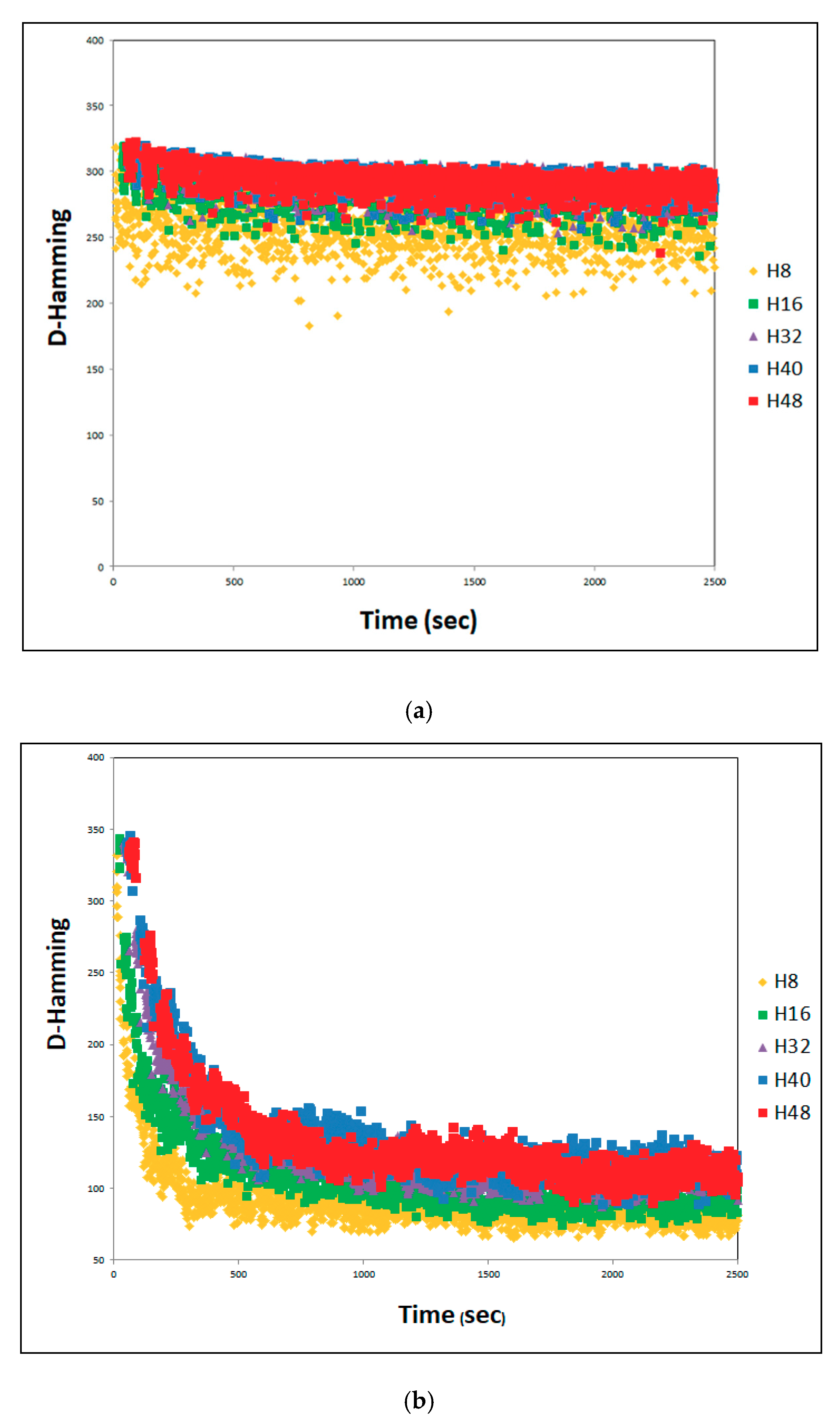
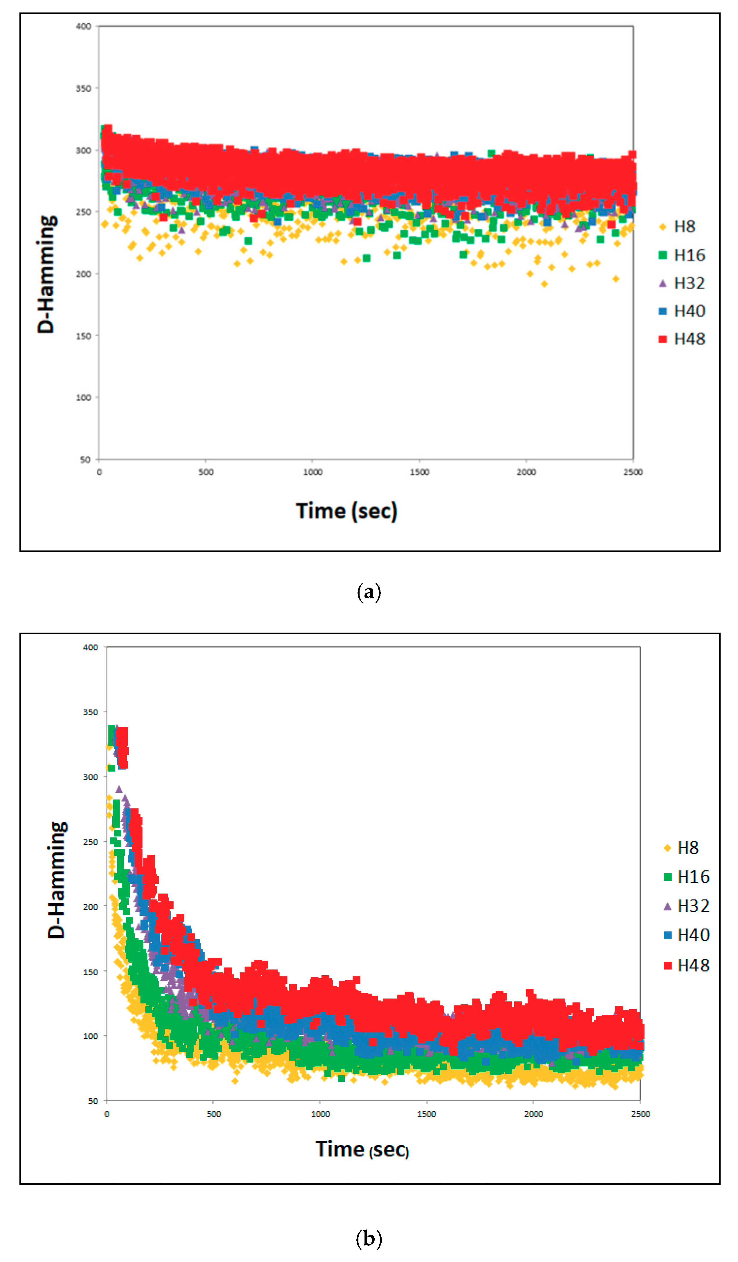
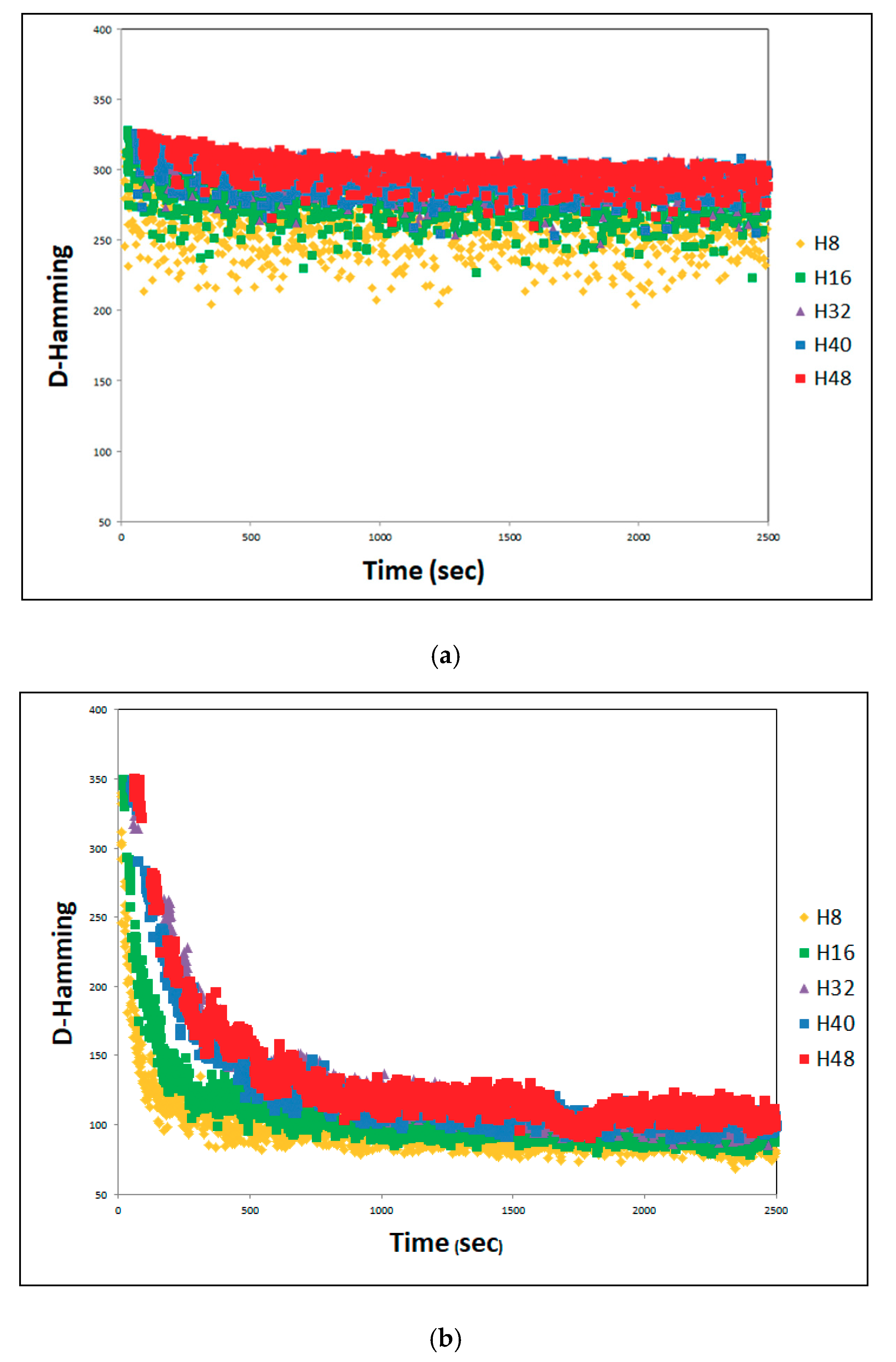
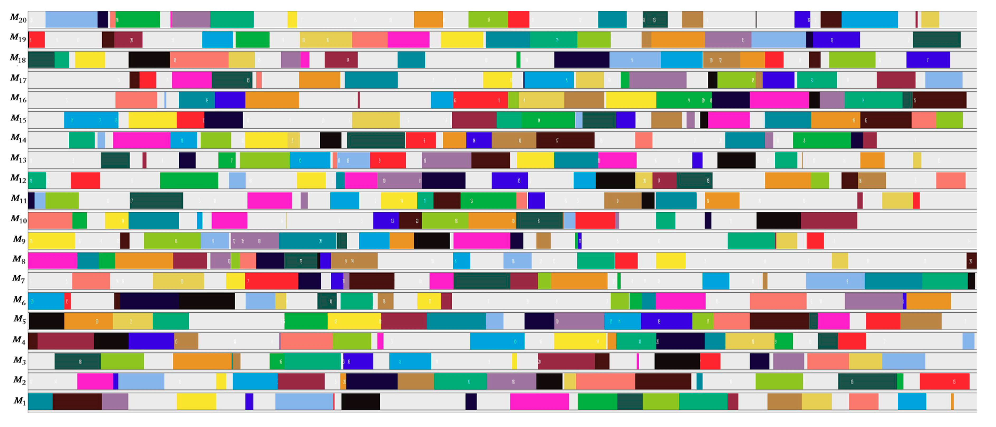
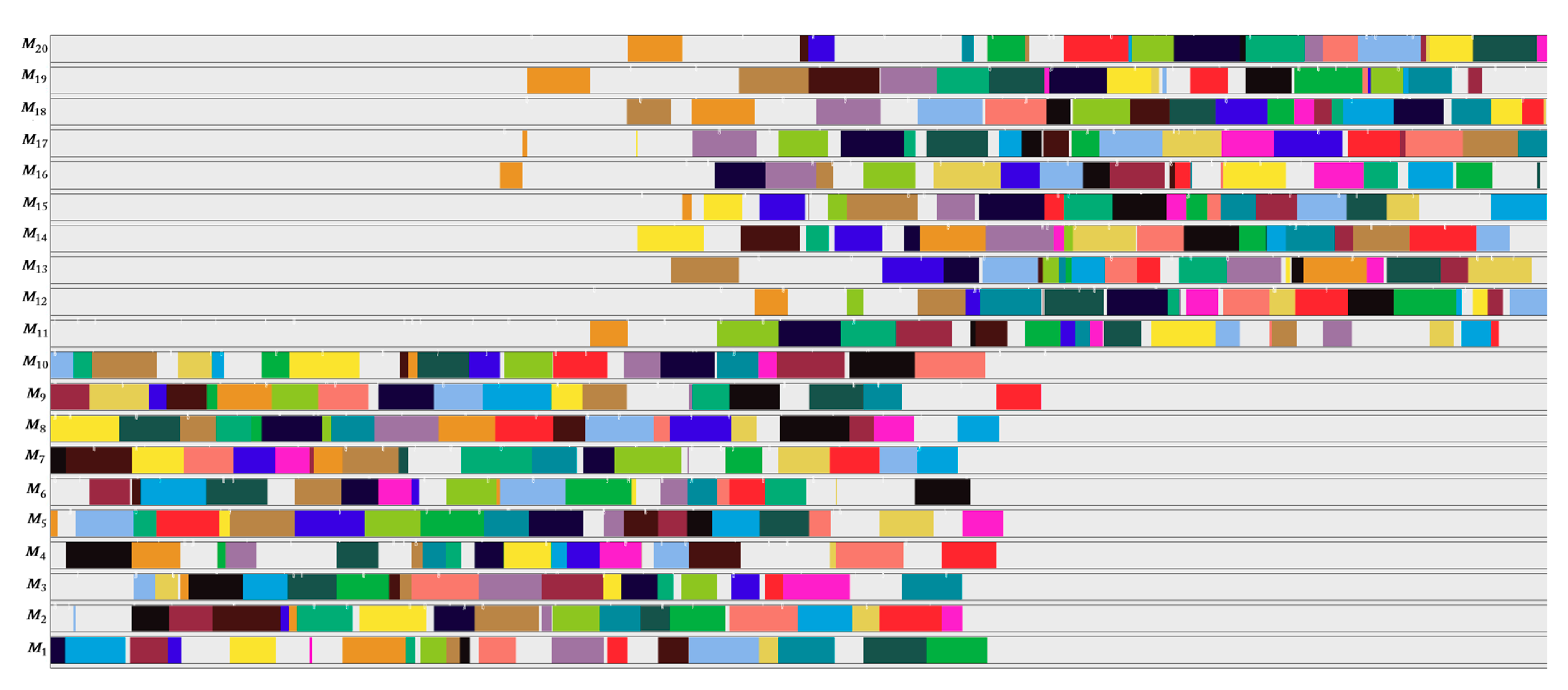
4.2. Effect of Cooperating with Effective-Address

In this paper, two different types of cooperation are utilized. In the first type of cooperation, SACT uses an effective-address procedure between two solutions with the best global solution S_best obtained from all threads. The best solution in the running thread is S_{Hi_c}, i.e., S_Hi = effective-address (S_{Hi_c}, S_best). With solution S_Hi obtained in each thread Hi, SA is restarted in each thread Hi. The second type of cooperation does not use effective-address in the SACT procedure for restarting SA in each thread Hi. Instead, S_Hi = S_{Hi_c} is used. In addition, in each iteration of SACT, the best solution S_best is saved. Cooperation occurs because the n threads working in parallel to find a solution at different points in the solution space always keep the best solution found in S_best.

In both types of cooperation, the best global solution S_best is obtained for each iteration of SACT because the best solution found in all threads for each SA is compared with the current best global solution, and the best solution S_best is saved.

The SACT algorithm was executed with several different numbers of threads and with a maximum value of 2500 Maxiter SA, which corresponds to about an hour of runtime for a number of threads SA ≥ 8. Figure 4, Figure 5, Figure 6, Figure 7, Figure 8, Figure 9, Figure 10, Figure 11 and Figure 12 (Maxiter vs. S_best), present respectively the performance of the cooperation of threads in SA for the problems YN1, YN2, YN3, and YN4. These figures present the execution of SACT for 8, 16, 32, 40, and 48 threads.

Figure 4a, Figure 5a, Figure 6a and Figure 7a show the relationship with efficacy. When there is cooperation without using the effective-address procedure, it can be observed that the best result obtained when Maxiter reaches 2500 SA does not depend on the number of threads in execution in SACT. The value of the makespan is very similar for any number of threads. This may be because there is no direct way to arrive at the same solution.

Figure 4b, Figure 5b, Figure 6b and Figure 7b show the relationship with efficacy. It can be observed that the best result obtained within the Maxiter = 2500 SA, using the effective-address procedure, was when SACT used 48 threads. Figure 6b shows that in YN3, 48 threads compete with 40 threads to find the best solution. This indicates that with a greater number of threads, on average, better solutions may be obtained. This effect is seen because the larger group of threads (H48) has the same directed pathway toward the same S_best solution. This is due to the greater number of effective-address applied to the n threads with the best solution S_best. The result is that a greater number of threads lead to a directed path through the best solution S_best. The Hamming distance becomes smaller between the set of threads with respect to S_best. This can be seen in Figure 8b, Figure 9b, Figure 10b and Figure 11b. It is generally observed in all cases that on average, the Hamming distance decreases with an increasing number of threads. Interestingly, with regard to the efficacy of the algorithm that can be noted in Figure 4b and Figure 7b for all other threads (H8, H16, H32, and H40), there is no defined behavior. For example, the efficacy as a function of the number of threads for YN1 (Figure 4b) in increasing order is H40, H8, H16, H32, H48. Efficacy as a function of the number of threads for YN2 (Figure 5b) in increasing order is H8, H16, H32, H40, H48. Efficacy as a function of the number of threads and YN3 (Figure 6b) in increasing order is H8, H16, H32, H48, H40. Efficacy as a function of the number of threads for YN4 (Figure 7b) in increasing order is H40, H16, H8, H32, H48. It can be seen that the efficacy of the algorithm SACT based on the number of threads, depends on the problem to solve. However, it can be observed that for all problems YN, generally with 48 threads, the efficacy of SACT is better in almost all YN; the average efficacy is better using 48 threads (H48).

Figure 4b, Figure 5b, Figure 6b and Figure 7b show that the worst behavior occurs when SACT is executed in a single thread sequence (H1) where cooperation with the effective-address procedure is with the only thread that exists (H1). It is noted that approximately from iteration = 100 SA, the efficiency decreases considerably for finding a good makespan when H8 is compared to H48. This behavior occurs for the four problems YN. The opposite happens when there is cooperation thread (H8 to H48). Efficacy increases on average from Figure 4b, Figure 5b, Figure 6b and Figure 7b, by about 10 units from iteration 250 to 2500 SA. This makes these makespan results better than those found by H1. For example, in YN1 of Figure 4b, in iteration 500 SA, the best average makespan when there is cooperation (H32) is close to 898. When there is no cooperation (H1), the makespan is about 909. In the iteration 2500 SA, the average makespan when there is cooperation (H48) is close to 894 and when there is no cooperation (H1), the makespan is close to 906.

Figure 4a, Figure 5a, Figure 6a and Figure 7a show that the worst performances are when SACT is executed in a single thread sequence (H1), where cooperation does not use the effective-address procedure. When the only thread that exists is (H1), the best solution is taken from the previous SA (S_H1 = S_{H1_c}). It is noted that approximately at the beginning (before Maxiter = 50 SA), the efficacy of H1 is better. Then this efficacy decreases considerably. This behavior occurs in all four YN problems. The opposite happens when there is cooperation thread (H8 to H48). The efficacy of cooperation increases as the number of iterations increases of 250–500 SA, as shown by better results for the makespan as compared to that found by H1. For example, in YN1, Figure 4a, at iteration 500 SA, the average makespan when there is cooperation (H8) is close to 902 and when there is no cooperation (H1), the makespan is about 908. In iteration 2000 SA, the average makespan when there is cooperation (H40) is close to 896 and when there is no cooperation (H1), the makespan is near 906.

An interesting point related to the efficacy of the SACT algorithm is that when there is cooperation but no effective-address there is no defined behavior for different threads in execution, as seen in Figure 4a, Figure 5a, Figure 6a and Figure 7a.

Table 2. Efficacy of SACT with cooperation and without effective-address procedure as a function of the threads executed.

Problem	Threads
	$\mathit{B}\mathit{e}\mathit{s}\mathit{t} \to \mathit{W}\mathit{o}\mathit{r}\mathit{s}\mathit{t}$
YN1	H40–H16	H16	H48	H8	H32	H1
YN2	H40–H32	H32	H8	H48	H16	H1
YN3	H32	H48	H40	H16	H8	H1
YN4	H16	H32	H40	H48	H8	H1

summarizes the efficacy of SACT with cooperation and without effective-address for YN problems in descending order. It can be observed that the efficacy of the algorithm SACT as a function of the number of threads depends on the problem being resolved. When there is both cooperation and effective-address, there is definite behavior for running threads, as can be seen in Figure 4b, Figure 5b, Figure 6b and Figure 7b.

Table 3. Efficacy of SACT with cooperation and with effective-address procedure as a function of the threads executed.

Problem	Threads
	$\mathit{B}\mathit{e}\mathit{s}\mathit{t} \to \mathit{W}\mathit{o}\mathit{r}\mathit{s}\mathit{t}$
YN1	H48	H32	H16	H8	H40	H1
YN2	H48–H40	H40	H32	H16	H8	H1
YN3	H40–H48	H48	H32	H16	H8	H1
YN4	H48	H32	H8	H16	H40	H1

presents the efficacy of SACT with cooperation and effective-address for YN problems in descending order. It can be seen that the increased efficacy of the SACT algorithm, as a function of the number of threads, occurs when the number of threads is the largest (H48). The exception to this is the YN3 problem, in which case the number of threads is also great. In YN1 and YN4, the worst efficacy is obtained with H40. According to

Table 4. SACT results, small benchmarks JSSP (10 × 10).

Problem	Optimum Units of Time	Better Units of Time	Worse Units of Time	Mean Units of Time	%RE	σ	t Sec	Median	Mode
FT6	55	55	55	55	0	0.0	0.03	55	55
FT10	930	930	930	930	0	0.0	1.05	930	930
LA16	945	945	945	945	0	0.0	5.1	945	945
LA17	784	784	784	784	0	0.0	4.9	784	784
L18	848	848	848	848	0	0.0	4.2	848	848
LA19	842	842	842	842	0	0.0	4.1	842	842
LA20	902	902	902	902	0	0.0	4.34	902	902
ORB01	1059	1059	1059	1059	0	0.0	13.63	1059	1059
ORB02	888	888	889	889	0	0.4	9720	889	889
ORB03	1005	1005	1021	1017	0	6.9	1048	1020	1021
ORB04	1005	1005	1005	1005	0	0.0	155	1005	1005
ORB05	887	887	890	888	0	1.6	1354	887	887
ORB06	1010	1010	1010	1010	0	0.0	59	1010	1010
ORB07	397	397	397	397	0	0.0	4.95	397	397
ORB08	899	899	899	899	0	0.0	10.33	899	899
ORB09	934	934	934	934	0	0.0	5	934	934
ORB10	944	944	944	944	0	0.0	4.84	944	944
ABZ5	1234	1234	1234	1234	0	0.0	12.62	1234	1234
ABZ6	943	943	943	943	0	0.0	4.23	943	943

, in order to define the number of threads needed to increase the efficacy in SACT, it would be necessary to start with H32 threads, and slowly increase the threads, being careful detect cases when SACT has a number of threads that presents a low efficacy, as in the case of YN1(H40) and YN4(H40).

An interesting point related to the efficacy of the SACT algorithm is that when there is cooperation but no effective-address there is no defined behavior for different threads in execution, as seen in Figure 4a, Figure 5a, Figure 6a and Figure 7a.

The efficacy of cooperation with the effective-address procedure (Figure 4b, Figure 5b, Figure 6b and Figure 7b), is noticed when, with a small number of iterations 500 SA, the value of an average makespan (MS) improves considerably when compared to the second type of cooperation (Figure 4a, Figure 5a, Figure 6a and Figure 7a). For example, for YN1 with effective-address, the average MS is about 900 (H8, H16, H32, H40, H48), as seen in Figure 4b. For YN1 without effective-address, the average MS is close to 905 (H8, H16, H32, H40, H48) as shown in Figure 4a. For YN2 with effective-address, the average MS is close to 922 (H8, H16, H32, H40, H48), as noted in Figure 5b. For YN2 without effective-address, the average MS is close to 928 (H8, H16, H32, H40, H48), as observed in Figure 5a.

For YN3, with effective-address, the average MS is close to 906 (H8, H16, H32, H40, H48), as seen in Figure 6b. For YN3 without effective-address, the average MS is close to 912 (H8, H16, H32, H40, H48), as shown in Figure 6a. For YN4 with effective-address, the average MS is close to 922 (H8, H16, H32, H40, H48), as noted Figure 7b. For YN4 without effective-address, the average MS is close to 928 (H8, H16, H32, H40, H48), as seen in Figure 7a. It can be observed that with a Maxiter = 500, the increased efficacy is almost constant for all YN, with 6 units of improvement in makespan when effective-address is used, as compared to when it is not used.

When comparing the first type of cooperation (Figure 4b, Figure 5b, Figure 6b and Figure 7b) and second type of cooperation (Figure 4a, Figure 5a, Figure 6a and Figure 7a), when the number of iterations is 2500, the average value of MS is better for the first type of cooperation. For YN1 with effective-address, the average MS is approximately 896 (H8, H16, H32, H40, H48), as seen in Figure 4b. For YN1 without effective-address, the average MS is approximately 898 (H8, H16, H32, H40, H48), as shown in Figure 4a. For YN2 with effective-address, the average MS is approximately 904 (H8, H16, H32, H40, H48), as noted in Figure 5b. For YN2 without effective-address, the average MS is approximately 905 (H8, H16, H32, H40, H48), as observed in Figure 5a. For YN3 with effective-address, the average MS is approximately 904 (H8, H16, H32, H40, H48), as seen in Figure 6b. For YN3 without effective-address, the average MS is approximately 905 (H8, H16, H32, H40, H48), as shown in Figure 6a. For YN4 with effective-address, the average MS is approximately 980 (H8, H16, H32, H40, H48), as observed in Figure 7b. For YN4 without effective-address, the average MS is approximately 985 (H8, H16, H32, H40, H48), as noted in Figure 7a. With a Maxiter = 2500, the increase in efficiency of the problem varies from 1 to 5 units of improvement in MS whether effective-address is used or not used. Even the slightest improvement in MS, which is 1, is very good, because what is sought with any optimization algorithm is to improve the bounds already known for big problems. The improved efficacy makes SACT competitive with the best algorithms reported in the literature, according to the results presented below.

Table 2 summarizes the efficacy of SACT with cooperation and without effective-address for YN problems in descending order. It can be observed that the efficacy of the algorithm SACT as a function of the number of threads depends on the problem being resolved. When there is both cooperation and effective-address, there is definite behavior for running threads, as can be seen in Figure 4b, Figure 5b, Figure 6b and Figure 7b.

Table 3 summarizes the efficacy of SACT with cooperation and with effective-address for YN problems in descending order. It can be seen that the increased efficacy of the SACT algorithm, as a function of the number of threads, occurs when the number of threads is the largest (H48). The exception to this is the YN3 problem, in which case the number of threads is also great. In YN1 and YN4, the worst efficacy is obtained with H40. According to Table 3, in order to define the number of threads needed to increase the efficacy in SACT, it would be necessary to start with H32 threads, and slowly increase the threads, being careful to detect cases when SACT has a number of threads that presents a low efficacy, as in the case of YN1(H40) and YN4(H40).

An evaluation of the Hamming distance presented in Figure 8, Figure 9, Figure 10 and Figure 11 for the problems YN1, YN2, YN3, and YN4, respectively, with different numbers of threads, shows the degree of similarity in each solution with respect to the best solution in each iteration. The Hamming distance between S_{Hi_c} and S_best is obtained by comparing the sequence of operations on each machine of JSSP. If the Hamming value of a solution S_{Hi_c} is zero regarding S_best, then the solution S_{Hi_c} is the same as S_best and they have the same configuration. Conversely, if S_{Hi_c}, has a very large Hamming value e.g., 400 (maximum value for a solution of the problem YN), then S_best is totally different from S_{Hi_c}. The greater the Hamming distance in a set of solutions S = {S_{H1_c}, S_{H2_c}, S_{H3_c}, ..., S_{Hn_c}} with respect to an S_best solution, the greater the diversity in the set of solutions S, where n is the number of running threads.

Figure 8a, Figure 9a, Figure 10a and Figure 11a, show that for cooperation without effective-address, more diversity exists than in the case of cooperation with effective-address. There is less diversity when movement follows a directed path via S_best, as seen in Figure 8b, Figure 9b, Figure 10b and Figure 11b.

In Figure 8a, Figure 9a, Figure 10a and Figure 11a, the Hamming distance without effective-address is within a range of 250 to 380. This is the case in almost all the execution interval of SACT, with different numbers of threads, and for different problems. It is true for YN1, YN2 between 180 and 325, YN3 between 190 and 320, and YN4 between 200 and 325. Given that in this kind of cooperation there is no effective-address, the diversity behavior remains almost constant throughout the runtime of SACT, with the exception of the first 250 s. It is seen that H8 and H16 have less diversity than all the other YN problems. Since there is not a directed path through the best solution S_best, the Hamming distance does not present a significant decrease over time. The behavior does differ in relation to the number of threads, as can be observed in Figure 8a, Figure 9a, Figure 10a and Figure 11a. In Figure 8a for YN1, the Hamming distance is greatest for H40 and least for H8. The other Hamming distances have almost the same average behavior (H16, H32, and H48).

In Figure 8a, Figure 9a, Figure 10a and Figure 11a, for YN2, YN3, and YN4, respectively, Hamming distance has the same average performance for H16, H32, H40, and H48. For H8, the Hamming distance is smaller. The behavior of the Hamming distance based on the number of threads is due to each thread involving a solution of SA. Because of this, if a larger number of solutions are compared to S_best, there could be a wider diversity. This is not always true because S_best has no relationship with most of the solutions generated by the thread. An example of this can be seen in Figure 8a, Hamming (H48) < Hamming (H40).

In Figure 8b, Figure 9b, Figure 10b and Figure 11b, the Hamming distance with effective-address at the beginning of SACT has a diversity of Hamming values up to 350. This is then reduced considerably as the execution progresses, and SACT has values in the range of 70 to 150. Because there is such cooperation with effective-address, the diversity is reduced because the search in the solution directs itself toward S_best solutions. The behavior of the Hamming distance based on the number of threads is due to each thread involving a solution of SA. Because of this, if a larger number of solutions are compared to S_best, there could be a wider diversity. However, as the time of implementation of effective-address, is reduced, solutions are directed toward a single path. This could be debatable. It can be observed in Figure 8b, Figure 9b, Figure 10b and Figure 11b and Figure 4b, Figure 5b, Figure 6b and Figure 7b, that applying cooperation threads with a directed path toward the best solution, a greater number of threads find better solutions. Since the greater diversity of the solutions is achieved with a greater number of threads, this avoids a hasty convergence prior to finding good solutions.

Figure 12 presents YN1 with H32 threads, with a long execution time of close to 2 h. It can be seen that the effective-address procedure still does not make the Hamming distance converge in SACT. What can be seen is that if SACT is left running an extremely long time, the Hamming distance will tend to zero.

The obtained results to YN problems indicate that in order for SACT to work with higher efficiency, it requires a computer that has a greater number of threads in order to allow SACT to make a greater number of effective-address with a greater number of threads, using a larger value of Maxiter.

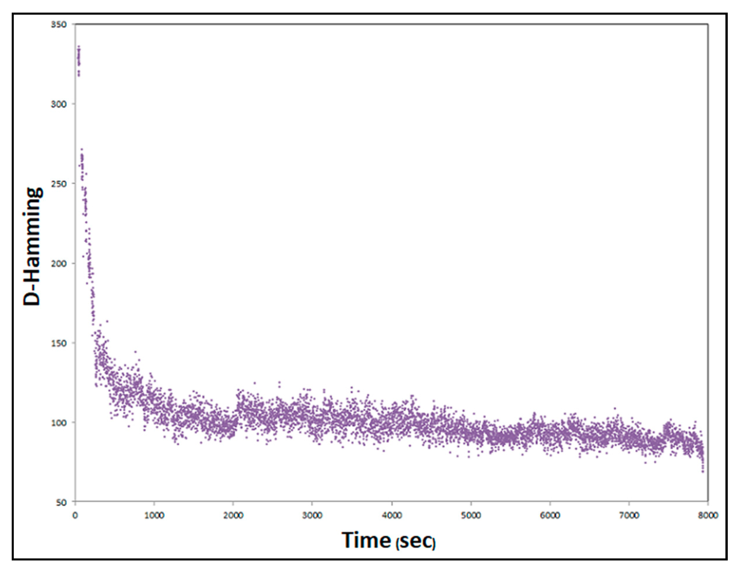
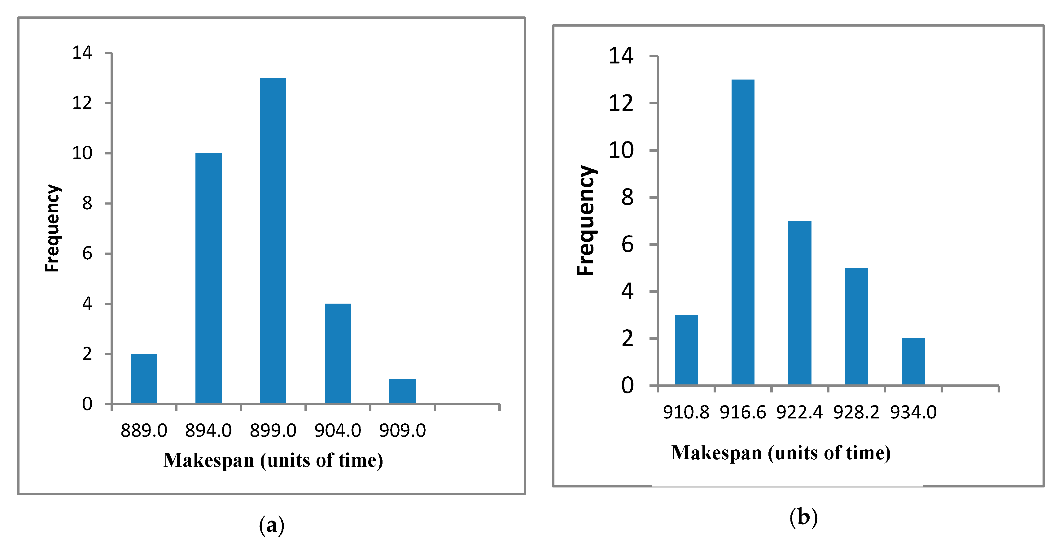
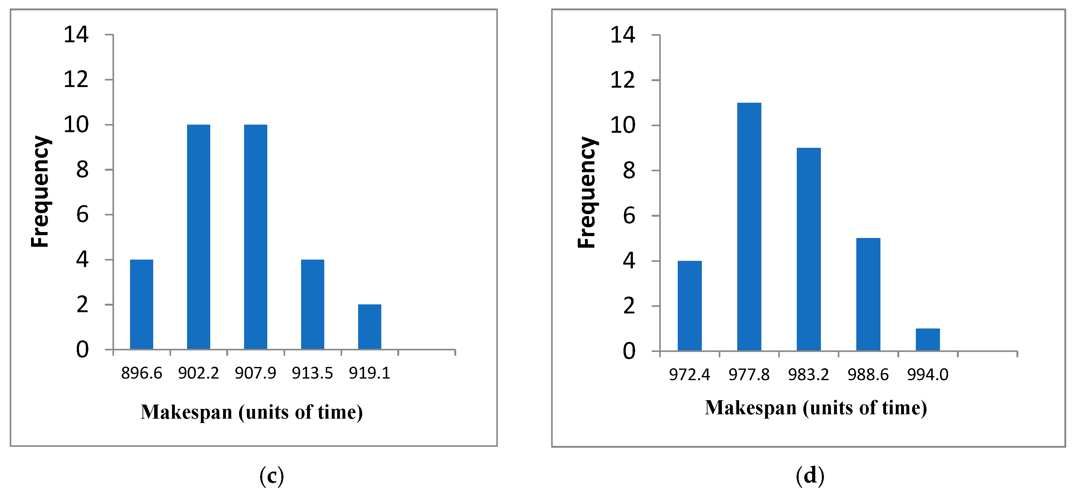
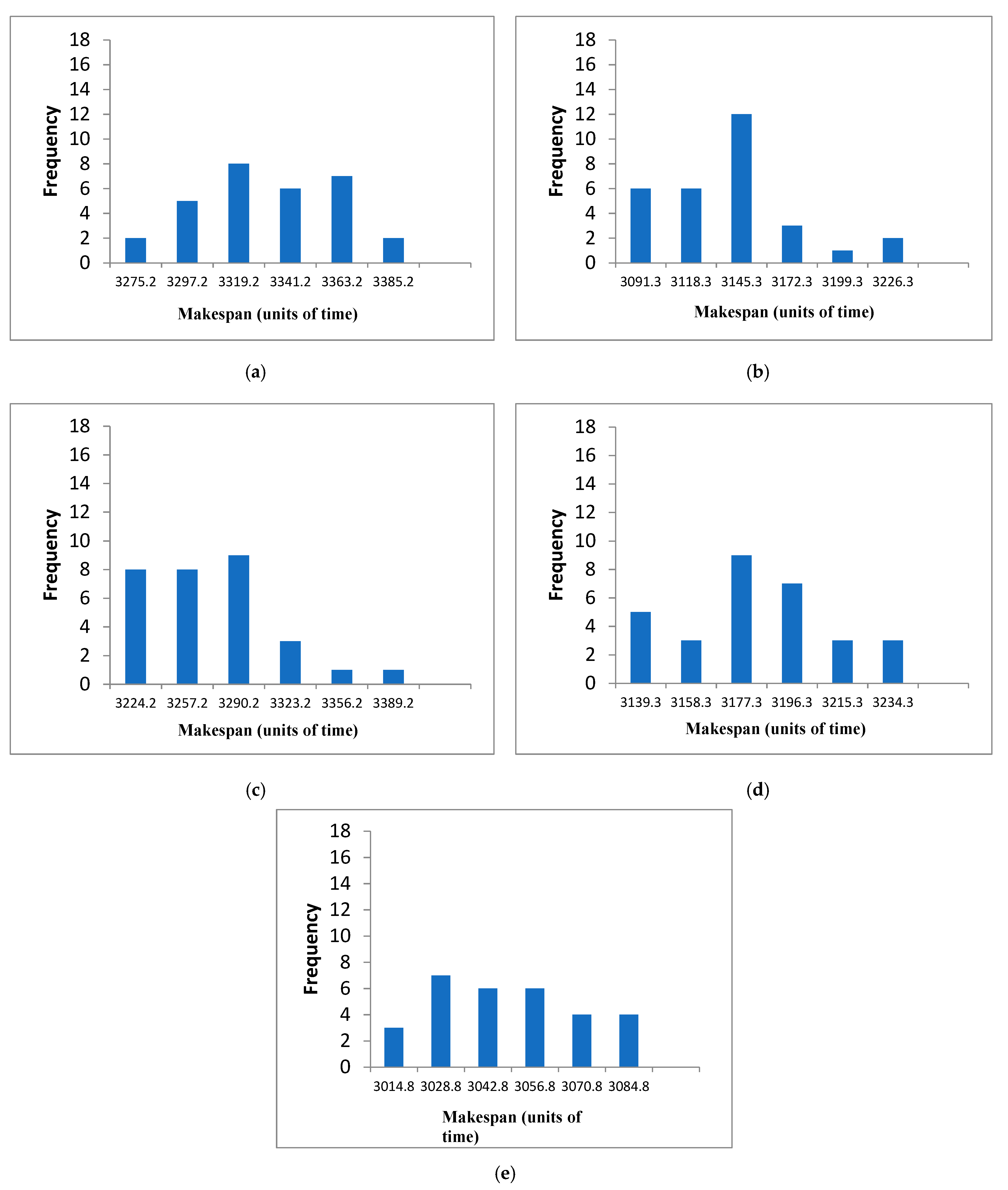
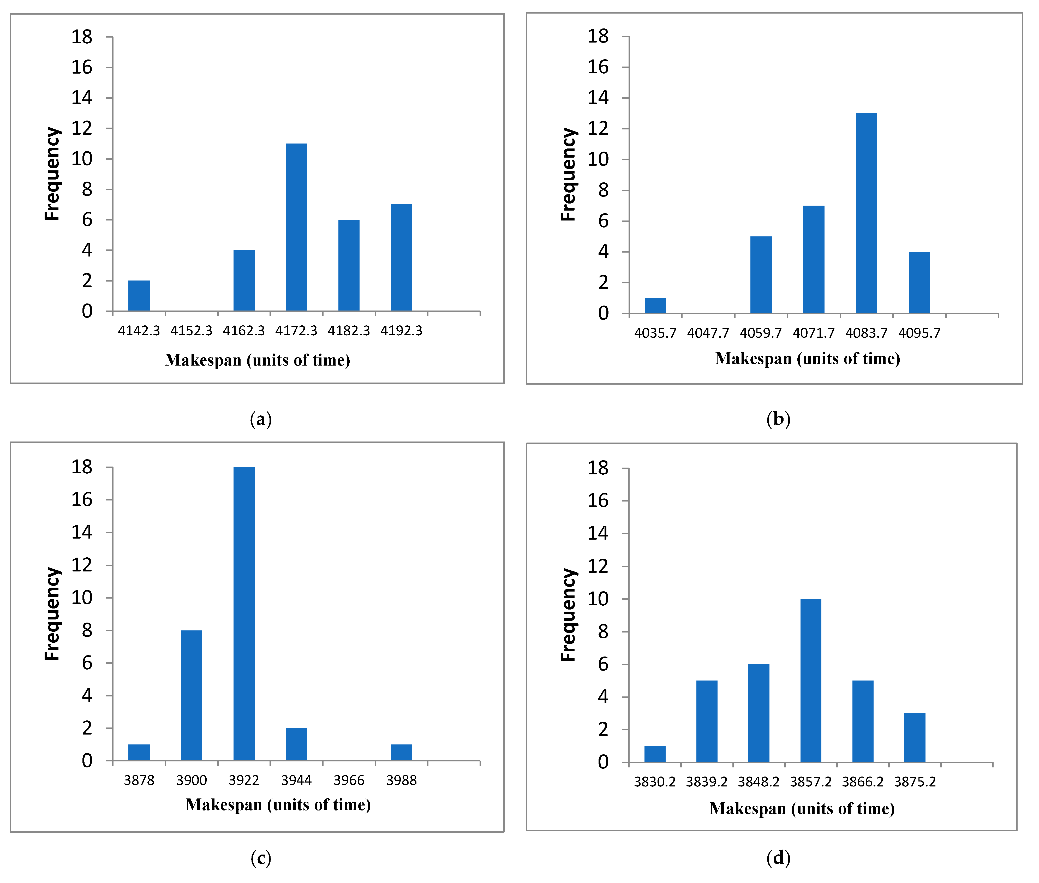
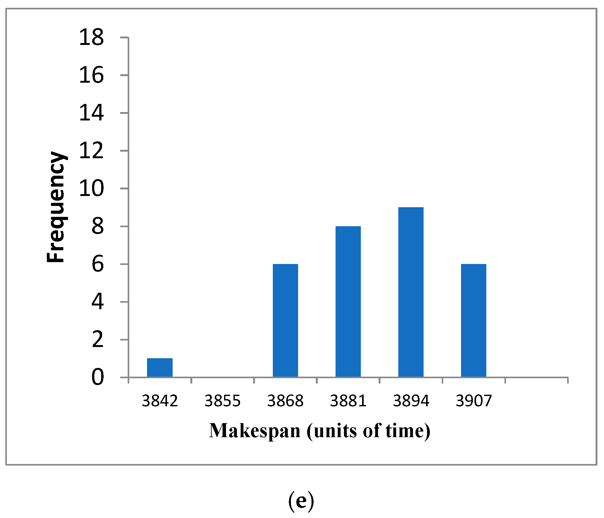
4.3. SACT Statistic Review

The bar plot is used in this paper as a tool to assess the frequency obtained from the solutions in terms of quality, the unit is no dimensional. The x-axis in the bar plot represents the value of the objective function of JSSP, which is the MS obtained by SACT.

Figure 13 shows the bar plots for YN1, YN2, YN3, and YN4 problems. In the four bar plots, SACT presents frequencies whose distribution is skewed to the left with respect to the midpoint.

The frequency distribution of YN1 and YN3 (Figure 13a,c) is very similar to a normal distribution. The frequency distribution of YN2 (Figure 13b) and YN4 (Figure 13d) is a little skewed to the right with respect to the midpoint (arithmetic mean), this is important because it indicates that most results obtained are to the left of the midpoint value, so the makespan found in most of the tests is of good quality. For YN1, 12 results out of 30 obtained, have a makespan value better or equal to the midpoint and are within the range 889–894. For YN2, 16 results out of 30 obtained, have a makespan value better or equal to the midpoint and are within the range 911–917. For YN3, 14 results out of 30 obtained, have a makespan value better or equal to the midpoint and are within the range 897–903. For YN4, 15 results out of 30 obtained, have a makespan value better or equal to the midpoint and are within the range 973–978. There is data concentration near the arithmetic mean for the four benchmarks, YN1 to YN4.

The frequency distribution of DMU06, DMU07, DMU08, and DMU10 (Figure 14) is skewed to the right with respect to the midpoint (arithmetic mean). DMU06 (Figure 14a) shows a bimodal frequency distribution, the highest frequency is 8 and is at the midpoint with 3319.2. At the left of the bar plot the frequency is 2 and the quality results is 3276. DMU07 (Figure 14b) and DMU08 (Figure 14c) present a data distribution further from the arithmetic mean, as opposed to DMU06, DMU09 (Figure 14d), and DMU10 (Figure 14e). For DMU07, 12 out of 30 results have a makepan value better or equal to the midpoint. At the far left of the bar plot the frequency is 6 and the quality results is 3092. At the far right of the bar plot the frequency is 2 and the quality results is 3227. DMU06 and DMU10 have a higher dispersion in the data distribution. For DMU08, 8 results of 30 obtained, have a makespan value better or equal to the midpoint and this value is 3225. At the far left of the bar plot the frequency is 8 and the quality results is 3225. At the far right of the bar plot the frequency is 1 and the quality results is 3390. For DMU09, 8 results out of 30 obtained, have a makespan value better or equal to the midpoint and are within the range 3140–3159. At the far left of the bar plot the frequency is 5 and the quality results is 3140. At the far right of the bar plot the frequency is 3 and the quality results is 3235. For DMU10, 10 results out of 30 obtained, have a makespan value better or equal to the midpoint and are within the range 3015–3029. At the far left of the bar plot the frequency is 3 and the quality results is 3015. At the far right of the bar plot the frequency is 4 and the quality results is 3085.

The frequency distribution of DMU46 and DMU47 (Figure 15) is skewed to the left with respect to the midpoint (arithmetic mean). For DMU48, the data are concentrated near the arithmetic mean, 26 out of 30. DMU50 has a central frequency distribution, with the exception of a single data that is far from this distribution. For DMU46 (Figure 15a), only 6 results out of 30 obtained, have a makespan value better or equal to the midpoint and are within the range 4143–4163. At the far left of the bar plot the frequency is 2 and the quality results is 4143. At the far right of the bar plot the frequency is 7 and the quality results is 4193. For DMU47 (Figure 15b), only 6 results out of 30 obtained, have a makespan value better or equal to the midpoint and are within the range 4036–4060. At the far left of the bar plot the frequency is 1 and the quality results is 4036. At the far right of the bar plot the frequency is 4 and the quality results is 4096. For DMU48 (Figure 15c), 9 results out of 30 obtained, have a makespan value better or equal to the midpoint and are within the range 3878–3900. At the far left of the bar plot the frequency is 1 and the quality results is 3878. At the far right of the bar plot the frequency is 1 and the quality results is 3988. For DMU49 (Figure 15d), 12 results out of 30 obtained, have a makespan value better or equal to the midpoint and are within the range 3831–3849. At the far left of the bar plot the best frequency is 1 and the quality results is 3831. At the far right of the bar plot the frequency is 3 and the quality results is 3876. For DMU50 (Figure 15e), 15 results out of 30 obtained, have a makespan value better or equal to the midpoint and are within the range 3842–3868. At the far left of the bar plot the best frequency is 1 and the quality results is 3842. At far right of the bar plot the frequency is 6 and the quality results is 3907.

The results obtained for the other small, medium, and large problems are presented in Table 4,

Table 5. SACT results, medium benchmarks JSSP (15 × 15).

Problem	Optimum Units of Time	Better Units of Time	Worse Units of Time	Mean Units of Time	%RE	σ	t Sec	Median	Mode
LA36	1268	1268	1281	1275	0	6.1	371.6	1278	1268
LA37	1397	1397	1399	1397	0	0.9	230	1397	1397
LA38	1196	1196	1245	1216	0	20.6	55	1218	1196
LA39	1233	1233	1237	1234	0	1.8	54	1233	1233
LA40	1222	1222	1234	1227	0	3.4	2245	1228	1229
TA01	1231	1231	1231	1231	0	0.0	328	1231	1231
TA02	1244	1244	1244	1244	0	0.0	501	1244	1244
TA03	1218	1218	1223	1221	0	2.3	4373	1221	1223
TA04	1175	1175	1175	1175	0	0.0	301	1175	1175
TA05	1224	1224	1231	1229	0	2.8	2218	1230	1230
TA06	1238	1238	1240	1239	0	0.8	5090	1239	1239
TA07	1227	1227	1228	1228	0	0.4	99	1228	1228
TA08	1217	1217	1224	1220	0	3.0	1986	1218	1218
TA09	1274	1274	1281	1277	0	3.6	1433	1274	1274
TA10	1241	1241	1253	1245	0	4.6	3830	1244	1244

and

Table 6. SACT results, large benchmarks JSSP (20 × 20).

Problem	UB Units of Time	Better Units of Time	Worse Units of Time	Mean Units of Time	%RE	σ	t Sec	Median	Mode
TA21	1642	1646	1772	1683	0.24	18.1	1938	1681	1665
TA22	1600	1600	1680	1637	0	13.1	3476	1636	1644
TA23	1557	1560	1628	1600	0.19	15.5	1681	1598	1598
TA24	1646	1651	1693	1681	0.3	14.4	397	1683	1670
TA25	1595	1597	1669	1633	0.13	17.9	2208	1634	1649
TA26	1643	1651	1716	1684	0.49	15.6	4547	1681	1680
TA27	1680	1682	1712	1701	0.12	6.5	1736	1700.5	1698
TA28	1603	1617	1639	1625	0.87	6.6	1374	1623	1622
TA29	1625	1627	1642	1631	0.12	4.9	4876	1628.5	1627
TA30	1584	1584	1618	1607	0	6.0	6429	1608.5	1606
DMU06	3244	3254	3381	3321	0.31	30.4	267	3319	3307
DMU07	3046	3065	3223	3127	0.62	37.5	3192	3122.5	3118
DMU08	3188	3192	3385	3255	0.13	41.8	1696	3253	3202
DMU09	3092	3121	3231	3174	0.94	29.5	1912	3173.5	3228
DMU10	2984	3001	3084	3042	0.57	23.1	246	3041	3032
DMU46	4035	4133	4189	4171	2.43	13.9	3424	4172	4176
DMU47	3942	4024	4094	4070	2.08	13.9	1244	4073.5	4074
DMU48	3763	3856	3988	3907	2.47	20.9	858	3906	3908
DMU49	3710	3822	3871	3851	3.02	21.3	8301	3906	3902
DMU50	3729	3829	3907	3882	2.68	16.2	5281	3881.5	3881
YN1	884	885	905	896	0.11	4.5	1558	895.5	896
YN2	904	906	930	917	0.22	6.4	3353	916	913
YN3	892	892	915	903	0	5.9	2459	903.5	904
YN4	968	968	990	978	0	5.8	3525	977.5	974

, respectively. The SACT used 48 threads. For each benchmark, 30 executions were carried out with SACT.

Table 4 presents the MS results with SACT for small benchmarks. For all the benchmarks the optimal solution value is reached (RE = 0). For most benchmarks the standard deviation of zero is obtained. The greatest standard deviation is obtained in ORB03 (σ = 6.9). For most benchmarks, the mode is the optimal solution obtained. The mode is the value that appears most often in the 30 tests. For most benchmarks, the median obtained is the optimal solution. If the median achieves the optimum, then at least half of the 30 tests achieved the optimal solution. The more difficult benchmarks that obtained the optimal solution according to the mode and median were ORB02 and ORB03. Table 4 shows, based on the standard deviation that the data distribution in each benchmark is completely homogeneous and the data are grouped very close to each other or with the same optimal value. For each benchmark in 30 tests, almost the same value for mean, median, and mode are found,, indicating a symmetrical distribution of data.

Table 5 presents the MS results with SACT for medium benchmarks. For all the benchmarks, the optimum value is reached (RE = 0). For most benchmarks, a small value of standard deviation (σ < 7) is obtained. The exception is the LA38 problem with the highest standard deviation of 21; however, this value is less than half of the arithmetic mean (mean) and this represents little dispersion of the data, however the dispersion of the data found by SACT in a frequency distribution for medium-sized benchmarks, is greater than the dispersion found for small-sized benchmark data. LA29 finds the optimal solution in 54 s. LA40 finds in 37 min. TA07 finds the optimal solution in 99 s and TA07 finds in 85 min. More than half of the benchmarks of medium size have a mode equal to the optimal solution. For most benchmarks, the median obtained is not the optimal solution. The most difficult problems for obtaining the optimal solution according to the mode and median were the benchmark LA40, TA03, TA05 to TA08, and TA10. LA40 was the most complicated of these benchmarks, the optimal solution was obtained in only one of the 30 executions, where the median and mode were furthest from the optimal value. Table 5 shows, based on the standard deviation that the data distribution in each benchmark is completely homogeneous and the data are grouped very close to each other or with the same optimal value. LA38 presents the data a little more dispersed (σ = 20.6).

Table 6 presents the MS results with SACT for large benchmarks. Most of the obtained values are close to the upper bound (UB), four of the benchmarks achieve this value. TA28 finds the greatest relative error (RE = 0.87%). TA22, TA30, YN3, and YN4 find the lowest RE = 0. The DMU benchmarks (46–50) are an exception because DMU49 finds the largest RE = 3.06 and DMU47 finds the lowest RE = 2.08. The largest standard deviation was 41.8 for the problem DMU08, and the lowest standard deviation was 4.9 for the problem YN1; however, this value is less than half of the arithmetic mean (mean) and this represents little dispersion of the data, however the dispersion of the data found by SACT in a frequency distribution for large-sized benchmarks, is greater than the dispersion found for small-sized benchmark data and medium-sized benchmark data. The mean is greater than the median and mode for DMU06 to DMU08 and DMU10, but with very close values, indicating very little skewed frequency distributions (see Figure 14). With DMU09 the mean is between the median and the mode indicating that the frequency distribution is close to a symmetrical distribution (see Figure 14d). The mean is less than the median and mode for DMU46 to DMU47 and DMU49, but with very close values, indicating very little skewed frequency distributions (see Figure 15). With DMU48 the mean is between the median and the mode indicating that the frequency distribution is close to a symmetrical distribution without taking the atypical value of 3988 (see Figure 15c). With DMU50 the mean is greater than the median and the mode but with very close values, indicating that the frequency distribution is close to a symmetrical distribution without taking the atypical value of 3842 (see Figure 15e). The shortest time for TA benchmarks was for TA22 and the longest time was for TA30. The time for DMU benchmarks with the smallest relative error was for DMU08 and the time with the largest relative error was for DMU49. The shortest time for YN benchmarks with the smallest relative error was for YN3 and the longest time with the biggest relative error was for YN2.

Figure 16 presents the average of 5 tests of the relative error obtained for 15 × 15 problems. It can be noted that the maximum RE occurs in LA38 and was not greater than 1.7. The most difficult problem was LA40, however 5 trials show that the average RE was not greater than 0.5. For the other 15 × 15 problems, the maximum average RE is in the range 0 ≤ RE ≤ 0.6. The problems for which it was easiest to find the global optimum were TA01, TA02, and TA04. In all the tests, they had RE = 0, which is why they are not present in Figure 16.

Figure 17 presents the average of 30 tests of the relative error obtained for the YN problems. It can be observed that the maximum RE occurs in YN2 and was not greater than 1.7; this problem had more difficulty approaching the upper bound of agreement in Table 6. The lowest average RE was in YN4, not greater than 1.2 with respect to the upper bound in Table 6.

Figure 18 presents the average of 30 tests of the relative error obtained for the DMU (06–10) problems. It can be observed that the maximum RE occurs in DMU07 and was not greater than 2.7. The DMU10 reached lowest average RE < 2. DMU08 was easier to approach the upper bound of agreement in Table 6. For the other DMU problems, the maximum average RE is in the range 2.3 < RE < 2.7.

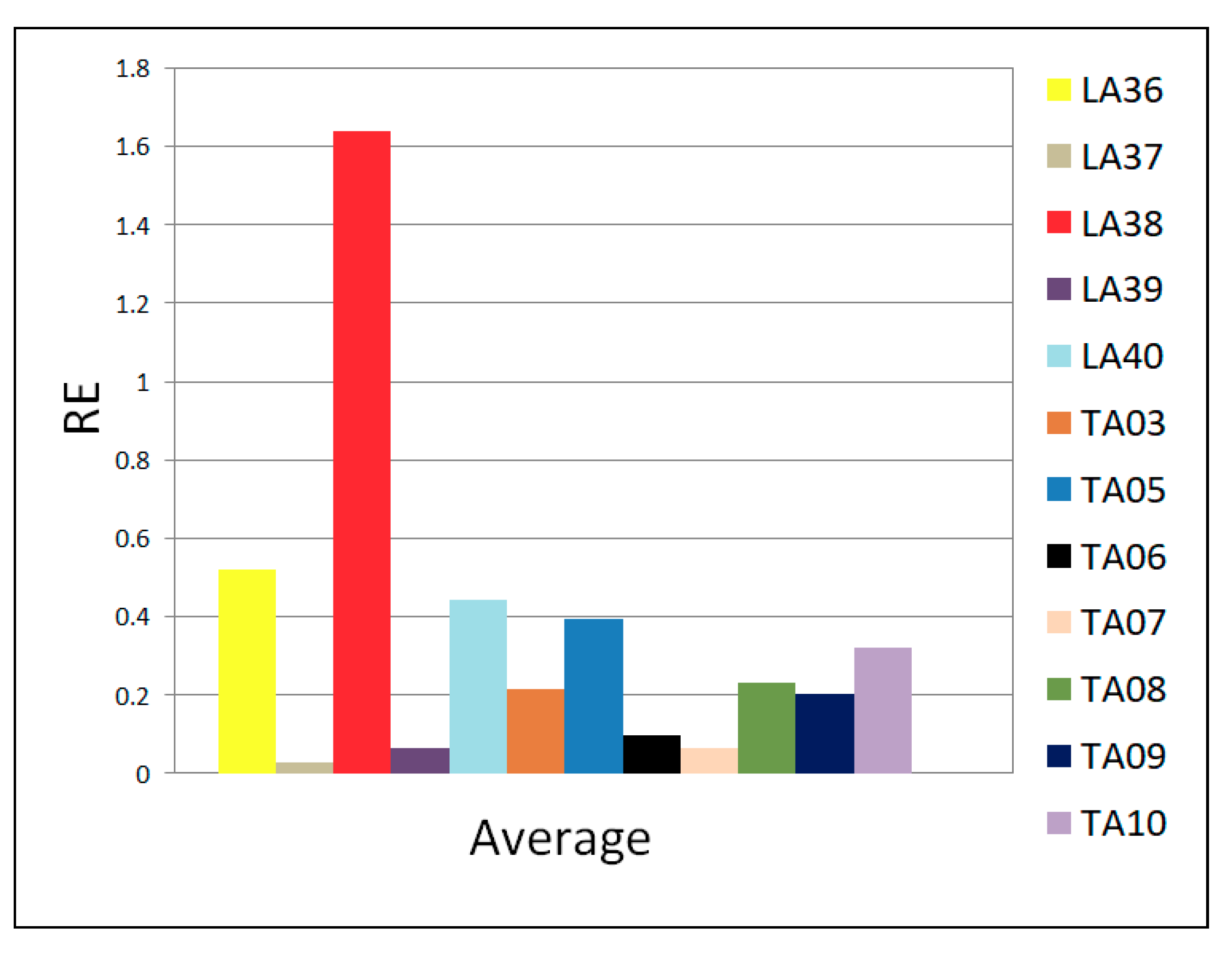
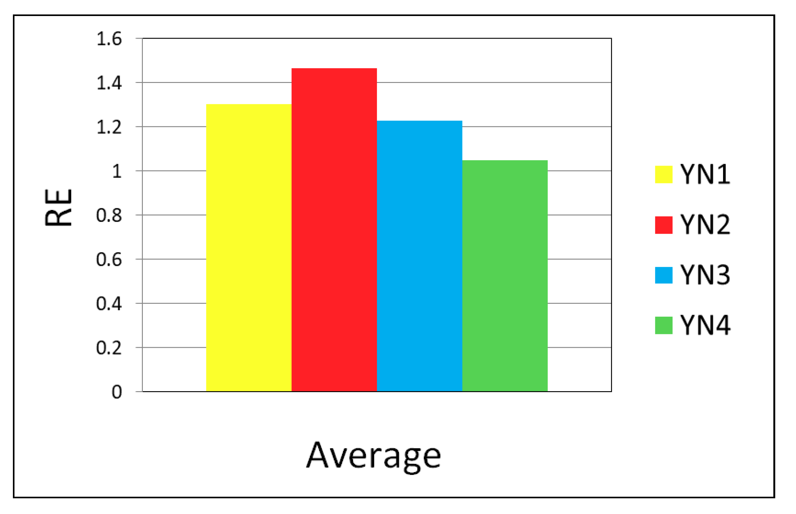
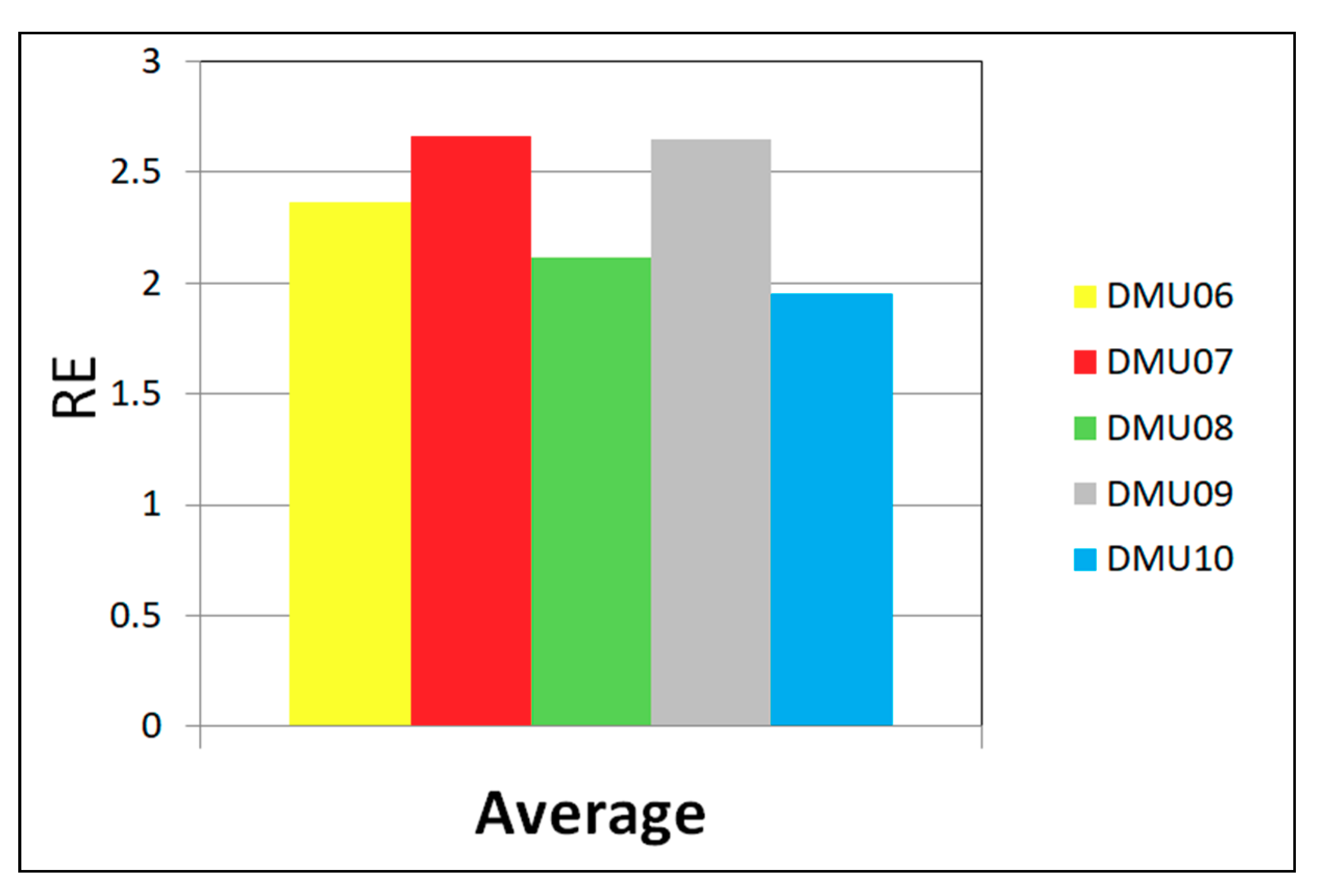
4.4. Behaviour in DMU Benchmarks Scheduling

Figure 19, presents the Gantt chart of the problem DMU08. The scheduling of the jobs in each of the problem’s machines can be observed. This type of distribution in the scheduling is characteristic of all problems, TA (21–30), YN (1–4), and DMU (06–10). The DMU problems (49–50) show different behavior. The scheduling distribution type is different. This is shown in Figure 20, where the Gantt diagram of the DMU46 problem is presented as an example.

Figure 20 shows that the planning of the job sequences in DMU46 indicates that in machines 1 to 10, the work operations can be sequenced from time zero. For machines 11 to 20, the operations of jobs cannot be sequenced at time zero because there is a precedence order in operations of the same job. This precedence order makes it impossible to use machines 11 to 20 if the operations of machines 1 to 10 have not previously been executed.

4.5. Comparision of SACT with Other Algorithms

Table 7. Efficiency and efficacy results for FT and LA benchmarks.

Prob	Op	ST	t Sec	BG	t Sec	SG	t Sec	AM	t Sec	TA	t Sec	SGS	t Sec	TGA	t Sec	TS/PR	t Sec	UP	t Sec	HO	t Sec	GT	AG
		%RE
Size 10 × 10
FT10	930	0	1.05	0	10.1	--	--	0	64.6	0	3.8	1.8	557	0	0.06	0	4.75	0	1208	0	4.1	0.54	0
LA16	945	0	5.1	0	4.6	0	38.8	--	--	--	--	0	304	0	0.094	0	0.15	0	1458	0	19.9	0.11	0.10
LA17	784	0	4.9	0	4.6	--	--	--	--	--	--	--	--	0	0.016	0	0.08	0	78	0	19.9	0	0
LA18	848	0	4.2	0	4.6	--	--	--	--	--	--	--	--	0	0.015	0	0.09	0	76	0	19.9	0	0
LA19	842	0	4.1	0	4.6	0	34.6	--	--	0	0.5	--	--	0	0.025	0	0.16	0	1130	0	19.9	0	1.18
LA20	902	0	4.34	0	4.6	--	--	--	--	--	--	--	--	0	0.031	0	0.11	0	1304	0	19.9	0.55	0.55
Size 15 × 15
LA36	1268	0	371.6	0	21.4	0	4655	0	36.6	0	9.9	--	--	0	0.57	0	4.5	0.79	48,387	0	105	3.16	--
LA37	1397	0	230	0	21.4	0.29	4144	0	879.6	0	42.1	--	--	0	0.51	0	26.2	0.72	49,836	0	105	6.59	--
LA38	1196	0	55	0	21.4	0.42	5049	0	55.4	0	47.8	--	--	0	1.25	0	32.6	1.59	50,876	0	105	6.61	--
LA39	1233	0	54	0	21.4	--	--	0	65.7	0	28.6	--	--	0	0.5	0	11.6	1.38	50,603	0	105	4.62	--
LA40	1222	0	2245	0	21.4	0.33	4544	0.16	941.4	0.16	52.1	--	--	0.16	0.86	0	385	0.57	50,609	0.16	105	2.46	--

, presents the results for the FT (Fisher and Thompson) and LA (Lawrence) benchmarks. SACT and BRK-GA (Biased Random-Key Genetic Algorithm) algorithms find the best results reported in the literature. Both algorithms obtained the optimal value for LA40. With regard to the execution time, it shows that SACT is competitive for most benchmarks.

Table A2. Software/hardware environment used in algorithms with which SACT is compared.

Algorithm	Hardware and Software
PPSO, [5]	Server and client Machines, Logical ring topology, Java, Windows system
HGAPSA, [14]	Server and client Machines
cGA-PR, [15]	Workstation Pentium IV, multicore, 2.0GHz, 1GB, Microsoft Visual C++
PaGA, [19]	Computer network with JADE Middleware, Java
HIMGA, [20]	PC, 3.4GHz, Intel®, Core(TM), i7-3770 CPU, 8GB, C++
NIMGA. PC, [21]	PC, 3.4GHz, Intel®, Core(TM), i7-3770 CPU, 8GB, C++
IIMMA, PC, [22]	PC, 3.4 GHz, Intel®, Core(TM), i7-3770 CPU, 8GB, C++
Sequential AntGenSA (SGS), Parallel AntGenSA (PGS), [23]	Cluster 4nodes, Intel® Xeon® 2.3 GHz, 64GB, Linux CentOS, C, OpenMP
PABC, [24]	Four computers system configuration, JAVA
HGACC (HG), [25]	CLUSTER, 48 cores, Xeon 3.06GHz, Linux Centos 5.5, GNU gcc, MPI Library
BRK-GA (BG), [36]	AMD Opteron 2.2GHz CPU, Linux Fedora release 12, C++
SAGen (SG), [37]	Pentium 120 (0.12 GHz), Pentium 166
ACOFT-MWR (AM), [38]	PC AMD 1533MHz CPU, 768 MB, Windows XP, Microsoft Visual C++ 6.0
TSSA (TA), [39]	PC Pentium IV 3.0GHz, Visual C++
HPSO (HO), [40]	PC, AMD Athlon 1700+ (1.47 GHz), Visual C++
TGA, [41]	PC 2.2 GHz, 8GB RAM, GNU gcc compiler
IEBO (IO), [42]	2.93 GHz, Intel Xeon X5670, GNU g++ compiler
TS/PR, [43]	PC Quad-Core AMD Athlon 3 GHz, 2GB, Windows 7, C++
UPLA, [44]	(UP) Intel CoreTM i5, processor M580 2.67 GHz, 6GB, C#
ALSGA (AG), [45]	Intel core 2 duo, 2.93 GHz, 2.0GB, Java Agent DEvelopment platform (JADE)
GA-CPG-GT (GT), [46]	PC 3.40 GHz Intel(R) Core (TM) i7-3770, 8GB, C++
SACT (ST), this work	Workstation PowerEdge T320, Intel® Xeon® Processor E5-2470 v2, 10cores, 3.10 GHz each, 24GB, Windows Vista Ultimate 64 bits O.S, Visual C++ 2008, MFC library

, in Appendix A, shows the software/hardware environment used for the execution of the algorithms presented in Table 7.

Table 8. Efficiency and efficacy for orb, ABZ, TA, DMU, and YN benchmarks.

Problem	Op/UB	ST	t Sec	BG	t Sec	AM	t Sec	TSSA	t Sec	SGS	T Sec	TGA	t Sec	IO	t Sec	TS/PR	t Sec	UP	t Sec	GT	AG
		%RE
Size 10 × 10
ORB01	1059	0	4.34	0	5.8	0	56.6	0	3.5	0	342	0	0.06	--	--	0	0.51	0	2312	2.36	3.12
ORB02	888	0	9720	0	5.8	0	569.3	0	6.4	0.1	306	0	0.06	--	--	0	1.69	0.11	2393	0.23	0.68
ORB03	1005	0	1048	0	5.8	0	403.7	0	13.8	1.2	330	0	0.15	--	--	0	1.46	0	2358	3.18	2.39
ORB04	1005	0	155	0	5.8	0	17.9	0	14.3	0	306	0	0.45	--	--	0	3.71	0	796	2.29	1.09
ORB05	887	0	1354	0	5.8	0	670.3	0	6.6	0	366	0	0.76	--	--	0	7.28	0.23	2458	0.79	1.58
ORB06	1010	0	59	0	5.8	--	--	0	8.5	--	--	0	0.72	--	--	0	1.81	0.30	2525	2.48	1.78
ORB07	397	0	4.95	0	5.8	--	--	0	0.5	--	--	0	0.02	--	--	0	0.13	0	2096	1.76	2.02
ORB08	899	0	10.33	0	5.8	--	---	0	7.2	--	--	0	0.09	--	--	0	3.99	0	2338	4.23	1.67
ORB09	934	0	5	0	5.8	--	--	0	0.4	--	--	0	0.09	--	--	0	0.47	0	884	0.96	0.96
ORB10	944	0	4.84	0	5.8	--	--	0	0.3	--	--	0	0.03	--	--	0	0.09	0	817	2.44	--
ABZ5	1234	0	12.62	--	--	0	501.9	--	--	--	--	0	0.04	--	--	--	--	--	--	0.32	--
ABZ6	943	0	4.23	--	--	0	199.3	--	--	--	--	0	0.03	--	--	--	--	--	--	0.42	--
Size 15 × 15
TA01	1231	0	328	0	30.4	0	1531.4	0	11.2	3.1	2782	--	--	0	124	0	2.93	--	--	--	--
TA02	1244	0	501	0	30.4	0	685.2	0	30.1	--	--	--	--	0	118	0	38	--	--	--	--
TA03	1218	0	4373	0	30.4	0.16	1833.7	0	108.5	--	--	--	--	0	120	0	44	--	--	--	--
TA04	1175	0	301	0	30.4	0	1186.2	0	71.7	--	--	--	--	0	117	0	39	--	--	--	--
TA05	1224	0	2218	0	30.4	0.33	1492.6	0	10.8	--	--	--	--	0	120	0	11	--	--	--	--
TA06	1238	0	5090	0	30.4	0	1549.1	0	125.2	--	--	--	--	0	113	0	178	--	--	--	--
TA07	1227	0.08	99	0.081	30.4	0.08	1687	0.08	138.6	--	--	--	--	0	117	0.08	0.60	--	--	--	--
TA08	1217	0	1986	0	30.4	0	968.4	0	27.6	--	--	--	--	0	108	0	2.43	--	--	--	--
TA09	1274	0	1433	0	30.4	0	1694.2	0	61.3	--	--	--	--	0	127	0	19	--	--	--	--
TA10	1241	0	3380	0	30.4	0	1418.2	0	68	--	--	--	--	0	122	0	42	--	--	--	--
Size 20 × 20
TA21	1642	0.24	1938	0	143.2	0.31	4158.4	0.12	437	--	--	--	--	0	408	0.12	503	--	--	--	--
TA22	1600	0	3476	0	143.2	0.06	3586.4	0	433.5	--	--	--	--	0	395	0	229	--	--	--	--
TA23	1557	0.19	1681	0	143.2	0.19	4175.7	0.19	429.4	--	--	--	--	0	390	0	360	--	--	--	--
TA24	1644	0.43	397	0.12	143.2	0.49	3320.2	0.12	431.6	--	--	--	--	0.12	435	0.06	779	--	--	--	--
TA25	1595	0.13	2208	0	143.2	0.13	3654.3	0.13	421	--	--	--	--	0	414	0	416	--	--	--	--
TA26	1643	0.49	4547	0	143.2	0.55	3178.8	0.24	436.2	--	--	--	--	0	87	0.24	268	--	--	--	--
TA27	1680	0.12	1736	0	143.2	0.36	3523.8	0	447.8	--	--	--	--	0	423	0	255	--	--	--	--
TA28	1603	0.87	1374	0	143.2	0.94	3804.8	0	431.2	--	--	--	--	0	370	0.62	326	--	--	--	--
TA29	1625	0.12	4876	0	143.2	0.12	3324.9	0.12	426.2	--	--	--	--	0	396	0	94	--	--	--	--
TA30	1584	0	6429	0	143.2	0.69	4003.5	0	436.1	--	--	--	--	0	429	0	389	--	--	--	--
DMU06	3244	0.31	267	0	145.4	--	--	--	--	--	--	--	--	--	--	0.03	823	--	--	--	--
DMU07	3046	0.62	3192	0	145.4	--	--	--	--	--	--	--	--	--	--	0	361	--	--	--	--
DMU08	3188	0.13	1696	0	145.4	--	--	--	--	--	--	--	--	--	--	0	296	--	--	--	--
DMU09	3092	0.94	1912	0	145.4	--	--	--	--	--	--	--	--	--	--	0.07	148	--	--	--	--
DMU10	2984	0.57	246	0	145.4	--	--	--	--	--	--	--	--	--	--	0.03	253	--	--	--	--
DMU46	4035	2.43	3424	0	187.7	--	--	--	--	--	--	--	--	--	---	0	985	--	--	--	--
DMU47	3939	2.15	1244	0	187.7	--	---	--	--	--	--	--	--	--	--	0.08	829	--	--	--	--
DMU48	3763	2.47	858	0.48	187.7	--	-	--	--	--	--	--	--	--	--	0.40	939	--	--	--	--
DMU49	3710	3.02	8301	0.35	187.7	--	--	--	--	--	--	--	--	--	--	0	634	--	--	--	--
DMU50	3729	2.68	5281	0.08	187.7	--	--	--	--	--	--	--	--	--	--	0	610	--	--	--	--
YN1	884	0.11	1558	0	105.2	--	--	0	106.6	0.2	15,786	0.23	92.8	0	190	0	169	--	--		--
YN2	904	0.22	3353	0	105.2	--	--	0.33	110.4	4.4	14,586	0.77	13.1	0	197	0	202	--	--	--	--
YN3	892	0	2459	0	105.2	--	--	0	110.8	1.3	16,662	0.56	37.2	0	212	0	344	--	--	--	--
YN4	967	0.1	3525	0.1	105.2	--	--	0.21	108.7	2.17	14,752	0.83	114.1	0.10	---	0.10	321	--	--	--	--

, presents results for ORB, ABZ, TA, DMU, and YN benchmarks in [33]. SACT obtains the best results reported in the literature for most of the benchmarks. The relative error (RE) for ORB, ABZ, TA, YN, and DMU (06–10) benchmark is RE < 0.95%. For DMU (47–50,) benchmark is RE < 3.03%. This shows that SACT is competitive with respect to the other algorithms presented. In [36] the researchers report a new UB = 904 for the problem YN2; previously the known UB was 907. SACT finds a UB = 906. Although this is not the new value reported by [36], it was able to improve the UB known before 2014. In efficiency, SACT is competitive with the ACOFT-MWR (Ant Colony Optimization with Fast Taboo - Most Work Remaining) . The exception can be seen with BRK-GA algorithm for the DMU benchmarks, SACT is, 0.12 < RE < 3.04 and BRK-GA is, 0 ≤ RE < 0.49. Table A2, in Appendix A, shows the software/hardware environment used for the execution of the algorithms presented in Table 8.

Table 9. Parallel algorithms, efficacy for FT, LA, ORB, TA, DMU, and YN benchmarks.

Problem	Size	Op/UB	%RE
			SACT	PPSO	cGA-PR	PaGA	HGAPSA	HIMGA	NIMGA	IIMMA	PGS	PABC	HG
FT06	6 × 6	55	0	--	--	0	--	0	0	0	0	0	--
FT10	10 × 10	930	0	--	0	7.2	--	0	0	0	0.9	0	0
LA16	10 × 10	945	0	29	--	5.2	--	0	0.11	0	--	0	0
LA17	10 × 10	784	0	33	--	1.2	--	0	0	0	--	0	0
LA18	10 × 10	848	0	33	--	1.4	--	0	0	0	--	0	0
LA19	10 × 10	842	0	37	--	3.7	--	0	0	0	--	0	0
LA20	10 × 10	902	0	32	--	1.1	--	0	0.55	0	--	0.55	0
LA36	15 × 15	1268	0	65	--	--	0.87	0	1.97	0	--	--	0
LA37	15 × 15	1397	0	58	--	--	0.79	0	3.01	0	--	--	0
LA38	15 × 15	1196	0	68	1.0	--	1.92	0	2.17	0	--	--	0
LA39	15 × 15	1233	0	67	--	--	1.05	0	2.11	0	--	--	0
LA40	15 × 15	1222	0	68	1.31	--	1.56	0.16	1.96	0.16	--	--	0
ORB01	10 × 10	1059	0	--	0	8.5	--	0	0	0	0	--	0
ORB02	10 × 10	888	0	--	--	4.6	--	0	0.23	0	0.1	--	0
ORB03	10 × 10	1005	0	--	0	12.3	--	0	2.09	0	0	--	0
ORB04	10 × 10	1005	0	--	0	5.7	--	0	1.39	0	0	--	0
ORB05	10 × 10	887	0	--	--	5.5	--	0	0.68	0	0	--	0
ORB06	10 × 10	1010	0	--	--	4.0	--	0	0.20	0	--	--	0
ORB07	10 × 10	397	0	--	--	4.8	--	0	0	0	--	--	0
ORB08	10 × 10	899	0	--	0	12.4	--	0	1.11	0	--	--	0
ORB09	10 × 10	934	0	--	--	6.4	--	0	0.86	0	--	--	0
ORB10	10 × 10	944	0	--	0	--	--	0	--	0	--	--	0
TA21	20 × 20	1642	0.24	--	0.49	--	--	0.49	--	--	--	--	--
TA22	20 × 20	1600	0	--	0.38	--	--	--	--	--	--	--	--
TA23	20 × 20	1557	0.19	--	0.19	--	--	--	--	--	--	--	--
TA24	20 × 20	1646	0.3	--	0.36	--	--	--	--	--	--	--	--
TA25	20 × 20	1595	0.13	--	0.13	--	--	--	--	--	--	--	--
TA26	20 × 20	1643	0.49	--	0.55	--	--	--	--	--	--	--	--
TA27	20 × 20	1680	0.12	--	0.36	--	--	--	--	--	--	--	--
TA28	20 × 20	1603	0.87	--	0.87	--	--	--	--	--	--	--	--
TA29	20 × 20	1625	0.12	--	0.25	--	--	--	--	--	--	--	--
TA30	20 × 20	1584	0	--	0	--	--	--	--	--	--	--	--
DMU06	20 × 20	3244	0.31	--	0.52	--	--	--	--	--	--	--	0.74
DMU07	20 × 20	3046	0.62	--	1.15	--	--	--	--	--	--	--	0.59
DMU08	20 × 20	3188	0.13	--	0.53	--	--	--	--	--	--	--	0
DMU09	20 × 20	3092	0.94	--	0.13	--	--	--	--	--	--	--	0.59
DMU10	20 × 20	2984	0.57	--	0.84	--	--	--	--	--	--	--	0.10
YN1	20 × 20	884	0.11	--	2.49	--	--	1.01	--	0.22	1.4	--	0.23
YN2	20 × 20	904	0.22	--	1.77	--	--	0.99	--	0.55	1.2	--	0.33
YN3	20 × 20	892	0	--	1.01	--	--	0.90	--	0.34	0.9	--	0
YN4	20 × 20	967	0.1	--	1.45	--	--	0.93	--	0.21	1.76	--	0.21

, presents the relative error of algorithms with threads/processes for the FT, LA, ORB, TA, DMU, and YN benchmarks. SACT has better performance with respect to the other algorithms, except DMU09. SACT has a relative error in the range of 0 ≤ RE ≤ 0.94%, PPSO (Parallel Particle Swarm Optimization) has a relative error in the range of 29 ≤ RE ≤ 68%, CGA-PR (Coarse-Grained Genetic Algorithm with Path-Relinking) has a relative error in the range of 0 ≤ RE ≤ 2.49%, PaGA (Parallel Agent-Based Genetic Algorithm) has a relative error in the range of 0 ≤ RE ≤ 12.4%, HGAPSA (Hybridization of Genetic Algorithm with Parallel Implementation of Simulated Annealing) presents a relative error of 0.79 ≤ RE ≤ 1.92%, HIMGA presents 0 ≤ RE ≤ 1.01%, NIMGA presents 0 ≤ RE ≤ 3.01%, IIMMA presents 0 ≤ RE ≤ 0.55% and AGS presents 0 ≤ RE ≤ 1.76%. Concerning the HGACC distributed algorithm, SACT offers a better performance for YN benchmarks. It reaches the same effectiveness for 10 × 10 and 15 × 15 size benchmarks. Thus, it is best for the DMU06 benchmark and is competitive for the other DMU benchmarks. Table A2, in Appendix A, shows the software/hardware environment used for the execution of the algorithms presented in Table 9.

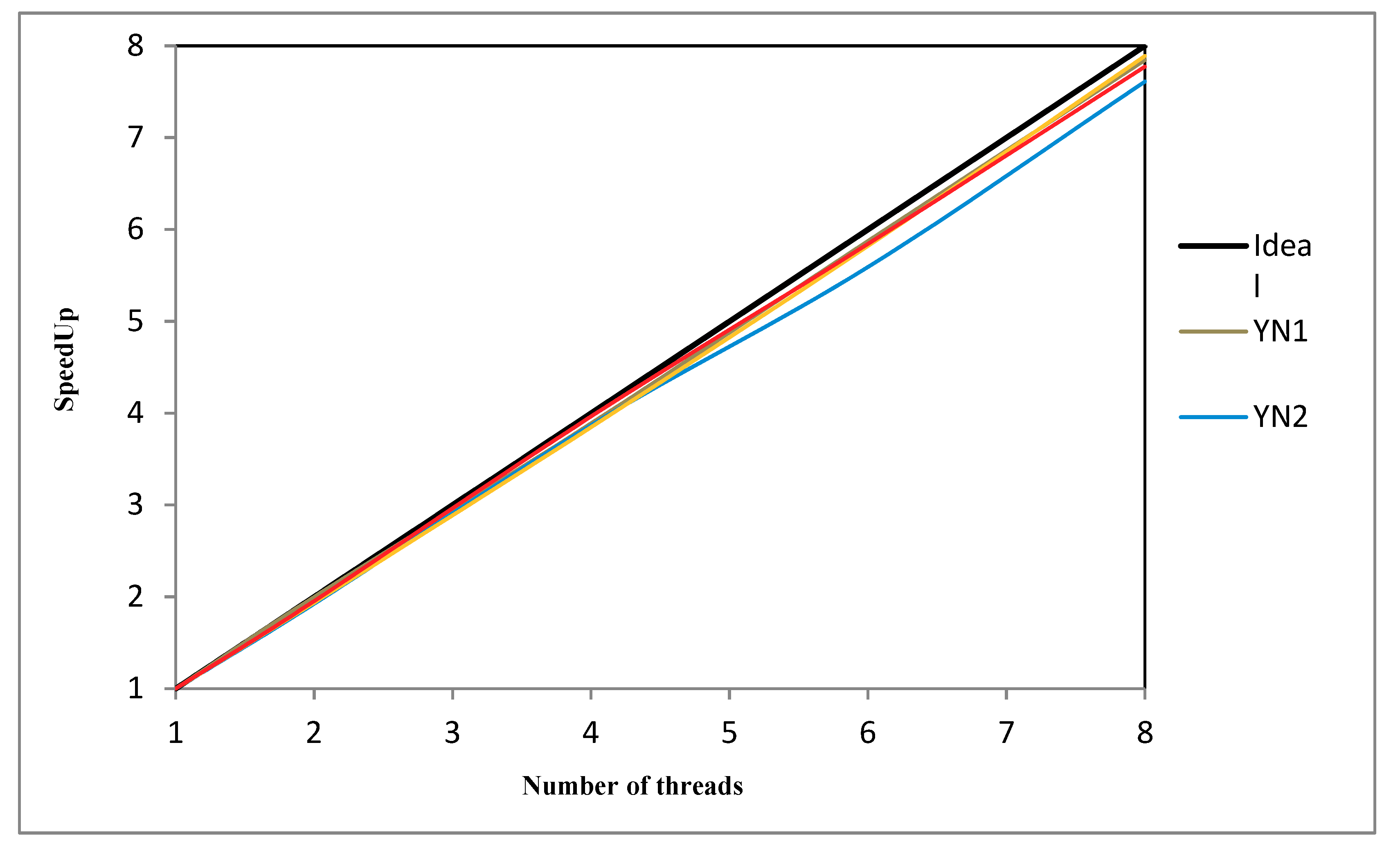
4.6. SACT Computational Efficiency

Figure 21 shows the SACT speedup for the YN benchmarks. The communication through cooperation between threads (access to the critical section) affects the speedup. An increased number of threads lead to greater cooperation because each running thread has the need to deposit the best solution in a critical section shared by all threads (see Figure 3), generating a bottleneck where in an instant of time the threads will have to wait their turn to access the critical section. This implies that increasing the number of threads will have a higher bottleneck, which results that the speedup moves away from the ideal. The speedup for YN2 is farthest from ideal with respect to other YN benchmarks. This may be because YN2 is taken more time to generate feasible solutions with the neighborhood generation mechanism [31]. So, it is possible that YN1, YN3, and YN4 will find solutions feasible faster. The neighborhood mechanism used in SACT is the only place in the algorithm that can perform differently on each benchmark. The speedup is very good for all YN benchmarks since is close to the ideal.

5. Conclusions

The study presented evidence that a benefit exists when the cooperation of threads is used applying effective-address procedure in the algorithm of simulated annealing for the job shop scheduling problem. It is also observed that the SACT algorithm can work more efficiently if it is executed in a computer with a greater number of threads per core. This permits an increase in the number of effective-address upon executing a greater number of SA in parallel.

Working with SACT in parallel allows the effective-address procedure to be efficiently applied because each thread constantly updates its search direction to a good solution space. In addition, no thread waits for any other thread in its simulated annealing run. That is why the search for better solutions between threads is asynchronous, enabling to run a larger number of simulated annealing compared to other threads, but always sharing the best solution space, and trying to improve the search direction with effective-address procedure on a constant basis. This makes the SACT algorithm more efficient if the number of threads is greater, which is reflected in the experimental results, as shown in Section 4.2.

According to the experimental results, it can be concluded that by applying cooperation threads with a directed path toward the best solution, a larger number of threads find best solutions. Since the diversity of solutions increases as the number of threads increases, a quick convergence before finding good solutions is avoided.

When the cooperation thread is applied without a directed path towards the same solution, finding a good result does not depend on the number of threads running on SACT. The value of the makespan is very similar for any number of threads.

The statistical review for the 19 small-sized benchmarks shows that SACT is highly effective since the optimal value is found in all instances. In 16 instances, the mean is the optimum, which indicates that for these instances, each of the 30 tests performed by SACT obtained the optimal value. According to the result of the median, it is understood that in 18 instances, the optimal solution is found in at least half of the 30 tests performed for each, which is reaffirmed by the mode of the same 18 instances.

The statistical review for the 15 medium-sized benchmarks shows that SACT is highly effective since the optimal value is found in all instances. In 4 instances, the mean is the optimum and this indicates that for these instances, each of the 30 tests performed by SACT obtained the optimal value. According to the result of the median, it is understood that in 5 instances, the optimal solution is found in at least half of the 30 tests performed for each. In 8 instances, the mode indicates that the optimal value is the one that appears more frequently.

The statistical review for the 20 large-sized benchmarks shows that SACT is very effective. In 4 instances, the upper bound is found and in 15 instances, the relative error does not exceed 1%.

Because the execution in SACT is executed by threads and communication in the algorithm handles only two critical sections, the efficiency (speedup) of the proposed algorithm is close to the ideal value. SACT also shows that efficacy is competitive when compared with other algorithms in the literature that have been very successful. Additionally, it is better than the algorithms in the literature that use threads/processes for the job shop problem.

Finally, the conclusion can be drawn that the optimum number of threads to execute in parallel by SACT is a parameter that must be tuned due to this cooperation in the threads.

The planning characteristics of the DMU (46–50) problems increase the degree of difficulty in obtaining good solutions by the proposed SACT algorithm. This is a topic of interest for future research, to search for an improved neighborhood mechanism that finds better solutions with the SACT algorithm for problems that behave like the DMU (46–50) problems with respect to the operation precedence and restrictions that prohibit starting all operations at time zero.

References

1. Garey, M.R.; Johnson, D.S. Computers and Intractability: A Guide to the Theory of NP-Completeness; W.H. Freeman and Company: New York, NY, USA, 1990; p. 340. [Google Scholar]
2. Perregaard, M.; Clausen, J. Parallel branch-and-bound methods for thejob-shop scheduling problem. Ann. Oper. Res. 1998, 83, 137–160. [Google Scholar]
3. Ku, W.-Y.; Beck, J.C. Mixed Integer Programming models for job shop scheduling: A computational analysis. Comput. Oper. Res. 2016, 73, 165–173. [Google Scholar] [CrossRef] [Green Version]
4. Dabah, A.; Bendjoudi, A.; El-Baz, D.; AitZai, A. GPU-Based Two Level Parallel B&B for the Blocking Job Shop Scheduling Problem. In Proceedings of the 2016 IEEE International Parallel and Distributed Processing Symposium Workshops (IPDPSW), Chicago, IL, USA, 23–27 May 2016; pp. 747–755. [Google Scholar]
5. AitZai, A.; Boudhar, M. Parallel branch-and-bound and parallel PSO algorithms for job shop scheduling problem with blocking. Int. J. Oper. Res. 2013, 16, 14. [Google Scholar] [CrossRef]
6. Der, U.; Steinhöfel, K. A Parallel implementation of a job shop scheduling heuristic. In Applied Parallel Computing. New Paradigms for HPC in Industry and Academia, PARA 2000; Sørevik, T., Manne, F., Gebremedhin, A.H., Moe, R., Eds.; Springer-Verlag: Berlin, Germany, 2001; pp. 215–222. [Google Scholar]
7. Steinhöfel, K.; Albrecht, A.; Wong, C. An experimental analysis of local minima to improve neighbourhood search. Comput. Oper. Res. 2003, 30, 2157–2173. [Google Scholar] [CrossRef]
8. Aydin, M.E.; Fogarty, T.C. A Distributed Evolutionary Simulated Annealing Algorithm for Combinatorial Optimisation Problems. J. Heuristics 2004, 10, 269–292. [Google Scholar] [CrossRef] [Green Version]
9. Skakovski, A.; Jędrzejowicz, P. An island-based differential evolution algorithm with the multi-size populations. Expert Syst. Appl. 2019, 126, 308–320. [Google Scholar] [CrossRef]
10. Yamada, T. A genetic algorithm with multi-step crossover for job-shop scheduling problems. In Proceedings of the 1st International Conference on Genetic Algorithms in Engineering Systems: Innovations and Applications (GALESIA), Sheffield, UK, 12–14 September 1995; pp. 146–151. [Google Scholar]
11. Yamada, T.; Nakano, R. A fusion of crossover and local search. In Proceedings of the IEEE International Conference on Industrial Technology (ICIT'96), Shanghai, China, 2–6 December 1996; pp. 426–430. [Google Scholar]
12. Nakano, R.; Yamada, T. Conventional genetic algorithm for job-shop problems. In Proceedings of the 4th International Conference on Genetic Algorithms, San Diego, CA, USA, July 1991; pp. 474–479. [Google Scholar]
13. Wendt, O.; König, W. Cooperative Simulated Annealing: How Much Cooperation Is Enough? Research Report; Frankfurt University: Frankfurt, Germany, 1997; pp. 1–19, unpublished. [Google Scholar]
14. Rakkiannan, T.; Palanisamy, B. Hybridization of Genetic Algorithm with Parallel Implementation of Simulated Annealing for Job Shop Scheduling. Am. J. Appl. Sci. 2012, 9, 1694–1705. [Google Scholar] [Green Version]
15. Spanos, A.C.; Ponis, S.T.; Tatsiopoulos, I.P.; Christou, I.T.; Rokou, E. A new hybrid parallel genetic algorithm for the job-shop scheduling problem. Int. Trans. Oper. Res. 2014, 21, 479–499. [Google Scholar] [CrossRef]
16. Yusof, R.; Khalid, M.; Hui, G.T.; Yusof, S.M.; Othman, M.F. Solving job shop scheduling problem using a hybrid parallel micro genetic algorithm. Appl. Soft Comput. 2011, 11, 5782–5792. [Google Scholar] [CrossRef]
17. Mùi, N.H.; Hòa, V.D.; Tuyên, L.T. A parallel genetic algorithm for the job shop scheduling problem. In Proceedings of the 2012 IEEE International Symposium on Signal Processing and Information Technology (ISSPIT), Ho Chi Minh City, Vietnam, 12–15 December 2012; pp. 19–24. [Google Scholar]
18. Yoo, M.J.; Müller, J.P. Using multi-agent system for dynamic job shop scheduling. In Proceedings of the 4th-ICEIS, Ciudad Real, Spain, 30 January 2002; pp. 1–8. [Google Scholar]
19. Asadzadeh, L.; Zamanifar, K. An agent-based parallel approach for the job shop scheduling problem with genetic algorithms. Math. Comput. Model. 2010, 52, 1957–1965. [Google Scholar] [CrossRef]
20. Beasley, J.E. OR-Library: Distributing Test Problems by Electronic Mail. J. Oper. Res. Soc. 1990, 41, 1069. [Google Scholar] [CrossRef]
21. Demirkol, E.; Mehta, S.; Uzsoy, R. A Computational Study of Shifting Bottleneck Procedures for Shop Scheduling Problems. J. Heuristics 1997, 3, 111–137. [Google Scholar] [CrossRef]
22. Watson, J.-P.; Beck, J.; Howe, A.E.; Whitley, L. Problem difficulty for tabu search in job-shop scheduling. Artif. Intell. 2003, 143, 189–217. [Google Scholar] [CrossRef] [Green Version]
23. Goncalves, J.F.; Resende, M.G.C. An extended akers graphical method with a biased random-key genetic algorithm for job-shop scheduling. Int. Trans. Oper. Res. 2014, 21, 215–246. [Google Scholar] [CrossRef]
24. Kolonko, M. Some new results on simulated annealing applied to the job shop scheduling problem. Eur. J. Oper. Res. 1999, 113, 123–136. [Google Scholar] [CrossRef]
25. Kuo-Ling, H.; Ching-Jong, L. Ant colony optimization combined with taboo search for the job shop scheduling problem. Comput. Oper. Res. 2008, 35, 1030–1046. [Google Scholar] [CrossRef]
26. Sha, D.; Hsu, C.-Y. A hybrid particle swarm optimization for job shop scheduling problem. Comput. Ind. Eng. 2006, 51, 791–808. [Google Scholar] [CrossRef]
27. Kurdi, M. A new hybrid island model genetic algorithm for job shop scheduling problem. Comput. Ind. Eng. 2015, 88, 273–283. [Google Scholar] [CrossRef]
28. Kurdi, M. An effective new island model genetic algorithm for job shop scheduling problem. Comput. Oper. Res. 2016, 67, 132–142. [Google Scholar] [CrossRef]
29. Kurdi, M. An improved island model memetic algorithm with a new cooperation phase for multi-objective job shop scheduling problem. Comput. Ind. Eng. 2017, 111, 183–201. [Google Scholar] [CrossRef]
30. Hernández-Ramírez, L.; Frausto-Solis, J.; Castilla-Valdez, G.; González-Barbosa, J.J.; Terán-Villanueva, D.; Morales-Rodríguez, M.L. A hybrid simulated annealing for job shop scheduling problem. Int. J. Comb. Optim. Probl. Inform. 2019, 10, 6–15. [Google Scholar]
31. Amirghasemi, M.; Zamani, R.; Amirghasemi, M. An effective asexual genetic algorithm for solving the job shop scheduling problem. Comput. Ind. Eng. 2015, 83, 123–138. [Google Scholar] [CrossRef] [Green Version]
32. Nagata, Y.; Ono, I. A guided local search with iterative ejections of bottleneck operations for the job shop scheduling problem. Comput. Oper. Res. 2018, 90, 60–71. [Google Scholar] [CrossRef]
33. Peng, B.; Lu, Z.; Cheng, T. A tabu search/path relinking algorithm to solve the job shop scheduling problem. Comput. Oper. Res. 2015, 53, 154–164. [Google Scholar] [CrossRef]
34. Cruz-Chávez, M.A. Neighborhood generation mechanism applied in simulated annealing to job shop scheduling problems. Int. J. Syst. Sci. 2015, 46, 2673–2685. [Google Scholar] [CrossRef]
35. Aksenov, V. Synchronization Costs in Parallel Programs and Concurrent Data Structures. Distributed, Parallel, and Cluster Computing [cs.DC]. ITMO University. Paris Diderot University. Available online: https://hal.inria.fr/tel-01887505/document (accessed on 4 October 2018).
36. Tanenbaum, A.S.; Bos, H. Modern Operating Systems, 4th ed.; Pearson Education: Amsterdan, The Netherlands, 2016; p. 1136. [Google Scholar]
37. Visual Studio 2019. MFC Desktop Applications. Available online: https://docs.microsoft.com/es-es/cpp/mfc/mfc-desktop-applications?view=vs-2019 (accessed on 27 July 2019).
38. Pongchairerks, P. A Two-Level Metaheuristic Algorithm for the Job-Shop Scheduling Problem. Complexity 2019, 2019, 8683472. [Google Scholar] [CrossRef]
39. Asadzadeh, L. A local search genetic algorithm for the job shop scheduling problem with intelligent agents. Comput. Ind. Eng. 2015, 85, 376–383. [Google Scholar] [CrossRef]
40. Kurdi, M. An effective genetic algorithm with a critical-path-guided Giffler and Thompson crossover operator for job shop scheduling problem. Int. J. Intell. Syst. Appl. Eng. 2019, 7, 13–18. [Google Scholar] [CrossRef] [Green Version]
41. Asadzadeh, L. A parallel artificial bee colony algorithm for the job shop scheduling problem with a dynamic migration strategy. Comput. Ind. Eng. 2016, 102, 359–367. [Google Scholar] [CrossRef]
42. Cruz-Chávez, M.A.; Cruz-Rosales, M.H.; Zavala-Díaz, J.C.; Hernández-Aguilar, J.A.; Rodríguez-León, A.; Prince-Avelino, J.C.; Luna, M.E.; Salina, O.H. Hybrid Micro Genetic Multi-Population Algorithm with Collective Communication for the Job Shop Scheduling Problem. IEEE Access 2019, 7, 82358–82376. [Google Scholar] [CrossRef]
43. Bryson, K. Global HPC Leaders Join to Support New Platform; NVIDIA: Santa Clara, CA, USA, 2019; Available online: https://nvidianews.nvidia.com/news/nvidia-brings-cuda-to-arm-enabling-new-path-to-exascale-supercomputing (accessed on 29 July 2019).
44. Lakin, D. How to Use the Same Thread Function for Multiple Threads (Safely). 2019. Available online: https://www.codeproject.com/Articles/1149/How-to-use-the-same-thread-function-for-multiple-t (accessed on 28 May 2001).
45. Amirghasemi, M.; Zamani, R. A synergetic combination of small and large neighborhood schemes in developing an effective procedure for solving the job shop scheduling problem. SpringerPlus 2014, 3, 193. [Google Scholar] [CrossRef] [PubMed] [Green Version]
46. Zhang, C.Y.; Li, P.; Rao, Y.; Guan, Z. A very fast TS/SA algorithm for the job shop scheduling problem. Comput. Oper. Res. 2008, 35, 282–294. [Google Scholar] [CrossRef]
Figure 1. Job shop scheduling with three jobs and three machines.
Applsci 09 03360 g001
Figure 2. Generation of neighbors.
Applsci 09 03360 g002
Figure 3. Communication of threads in SACT for sharing information using critical sections.
Applsci 09 03360 g003
Figure 4. YN1-20 × 20. Performance of cooperation with different numbers of threads. Average of 30 tests. (a) Without effective-address. (b) With effective-address.
Applsci 09 03360 g004
Figure 5. YN2-20 × 20. Performance of cooperation with different numbers of threads. Average of 30 tests. (a) Without effective-address. (b) With effective-address.
Applsci 09 03360 g005
Figure 6. YN3-20 × 20. Performance of cooperation with different numbers of threads. Average of 30 tests. (a) Without effective-address. (b) With effective-address.4.
Applsci 09 03360 g006
Figure 7. YN4-20 × 20. Performance of cooperation with threads. Average of 30 tests. (a) Without effective-address. (b) With effective-address procedure.
Applsci 09 03360 g007
Figure 8. YN1-20 × 20. Solution diversity with different number of threads. Average of 30 tests. (a) Without effective-address. (b) With effective-address.
Applsci 09 03360 g008
Figure 9. YN2-20 × 20. Solution diversity with different number of threads. Average of 30 tests. (a) Without effective-address. (b) With effective-address.
Applsci 09 03360 g009
Figure 10. YN3-20 × 20. Solution diversity with different number of threads. Average of 30 tests. (a) Without effective-address. (b) With effective-address.
Applsci 09 03360 g010
Figure 11. YN4-20 × 20. Solution diversity with different number of threads. Average of 30 tests. (a) Without effective-address. (b) With effective-address.
Applsci 09 03360 g011
Figure 12. Effect of the effective-address procedure on the convergence of SACT for long times. YN1-20 × 20. H32.
Applsci 09 03360 g012
Figure 13. SACT, bar plots YN1, YN1, YN3, YN4. (a) SACT, YN1 (30 tests). (b) SACT YN2 (30 tests). (c) SACT, YN3 (30 tests). (d) SACT, YN4 (30 tests).
Applsci 09 03360 g013aApplsci 09 03360 g013b
Figure 14. SACT bar plots DMU06, DMU07, DMU08, DMU09, DMU10. (a) SACT, DMU06 (30 tests). (b) SACT, DMU07 (30 tests). (c) SACT, DMU08 (30 tests). (d) SACT, DMU09 (30 tests). (e) SACT, DMU10 (30 tests).
Applsci 09 03360 g014
Figure 15. SACT bar plots DMU46, DMU47, DMU48, DMU49, DMU50. (a) SACT, DMU46 (30 tests). (b) SACT, DMU47 (30 tests). (c) SACT, DMU48 (30 tests). (d) SACT, DMU49 (30 tests). (e) SACT, DMU50 (30 tests).
Applsci 09 03360 g015aApplsci 09 03360 g015b
Figure 16. Relative error, average of five tests, JSSP 15 × 15.
Applsci 09 03360 g016
Figure 17. Relative error, average of thirty tests, JSSP 20 × 20.
Applsci 09 03360 g017
Figure 18. Relative error for thirty executions of problems DMU (06–10) of JSSP 20 × 20.
Applsci 09 03360 g018
Figure 19. Scheduling Gantt chart of the problem DMU08.
Applsci 09 03360 g019
Figure 20. Scheduling Gantt chart of the problem DMU46
Applsci 09 03360 g020
Figure 21. SACT algorithm, speedup for benchmarks 20 × 20 (YN1, YN2, YN3, and YN4).
Applsci 09 03360 g021