Special Issue on Using Machine Learning Algorithms in the Prediction of Kyphosis Disease: A Comparative Study

Abstract

Machine learning (ML) is the technology that allows a computer system to learn from the environment, through re-iterative processes, and improve itself from experience. Recently, machine learning has gained massive attention across numerous fields, and is making it easy to model data extremely well, without the importance of using strong assumptions about the modeled system. The rise of machine learning has proven to better describe data as a result of providing both engineering solutions and an important benchmark. Therefore, in this current research work, we applied three different machine learning algorithms, which were, the Random Forest (RF), Support Vector Machines (SVM), and Artificial Neural Network (ANN) to predict kyphosis disease based on a biomedical data. At the initial stage of the experiments, we performed 5- and 10-Fold Cross-Validation using Logistic Regression as a baseline model to compare with our ML models without performing grid search. We then evaluated the models and compared their performances based on 5- and 10-Fold Cross-Validation after running grid search algorithms on the ML models. Among the Support Vector Machines, we experimented with the three kernels (Linear, Radial Basis Function (RBF), Polynomial). We observed overall accuracies of the models between 79%–85%, and 77%–86% based on the 5- and 10-Fold Cross-Validation, after running grid search respectively. Based on the 5- and 10-Fold Cross-Validation as evaluation metrics, the RF, SVM-RBF, and ANN models achieved accuracies more than 80%. The RF, SVM-RBF and ANN models outperformed the baseline model based on the 10-Fold Cross-Validation with grid search. Overall, in terms of accuracies, the ANN model outperformed all the other ML models, achieving 85.19% and 86.42% based on the 5- and 10-Fold Cross-Validation. We proposed that RF, SVM-RBF and ANN models should be used to detect and predict kyphosis disease after a patient had undergone surgery or operation. We suggest that machine learning should be adopted and used as an essential and critical tool across the maximum spectrum of answering biomedical questions.

1. Introduction

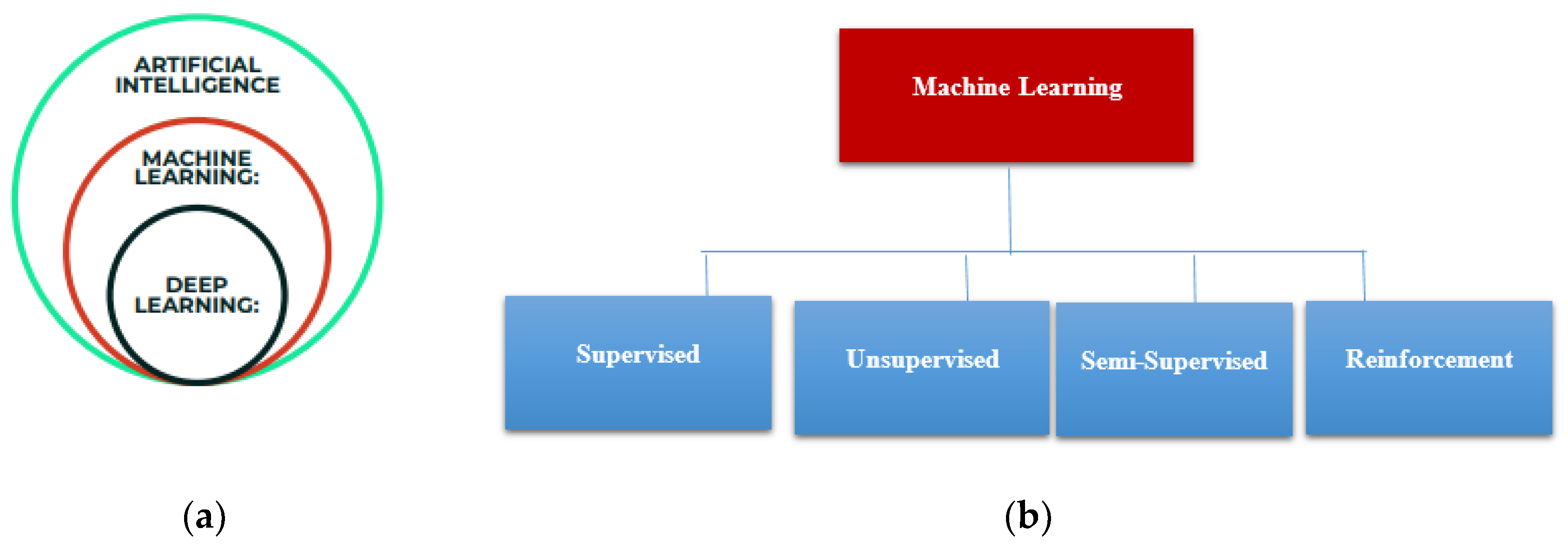
Machine learning is a subfield of Artificial Intelligence as shown in Figure 1a, that allows a computer system to learn from the environment, through re-iterative processes and improve itself from experience. Machine learning algorithms organize the data, learn from it, gather insights and make predictions based on the information it analyzed without the need for additional explicit programming. Training a model with data and after that using the model to predict any new data is the concern of machine learning. Machine learning algorithms are widely composed of supervised, unsupervised, semi-supervised, and reinforcement learning as shown in Figure 1b. In this current work, we focused on supervised learning, where there is a part of the training data which behaves as an instructor to the algorithm to determine the model.

The development of machine learning has proven to better describe data as a result of providing both engineering solutions and an important benchmark. According to Vinitha et al. [1], as a result of big data development in biomedical and healthcare communities, precise study of medical data benefits early disease recognition, patient care and community services.

Machine learning algorithms were developed with numerous features such as effective performance on healthcare related data that includes text, images, X-rays, blood samples etc. [2]. The choice of the algorithm to be used depends on the type of dataset, be it large or small. Sometimes the noise in a dataset can be a drawback to some machine learning algorithms [2]. Sometimes, after viewing a dataset, interpreting the pattern and extracting meaningful information becomes difficult, hence the need of machine learning [3,4]. At a regularization point where a model quality is highest, variance and bias problems are compromised, and that is where Random Forest (RF) model is used. Random Forest has the capability of building numerous numbers of decision trees using random samples with a replacement to overcome the shortcomings of the Decision tree algorithm.

Support Vector Machines (SVM) is a pattern classification technique which, when trained, has the capability to learn classification and regression rules from observation data [2,5]. Support Vector Machine theory is based on statistics which have a fundamental principle of estimating the optimal linear hyperplane in a feature space that maximally separates the two-mark groups or classes. Support Vector Machine algorithm shows the feasibility and superiority to extract higher-order statistics [6].

Artificial Neural Networks (ANNs) are computational models based on the neural structure of the brain. ANN has the capability of searching for patterns among patients’ healthcare and personal records to retrieve and identify meaningful information [2,7]. Application of machine learning algorithms in the medical field for disease diagnosis and prediction can help experts in disease identification depending on the symptoms at an early stage [8].

When it comes to diagnosing and predicting diseases using machine learning algorithms, especially on biomedical text datasets, several researchers have done significant work to predict other diseases such as diabetes [9], heart diseases [10,11,12,13,14,15], breast cancer disease [7,16,17], and even in the prediction of medical costs of Spinal Fusion [18], etc. However, to the best of our knowledge, much has not been explored in predicting kyphosis disease. Kyphosis is a dangerous disease and equally needs attention as the aforementioned diseases.

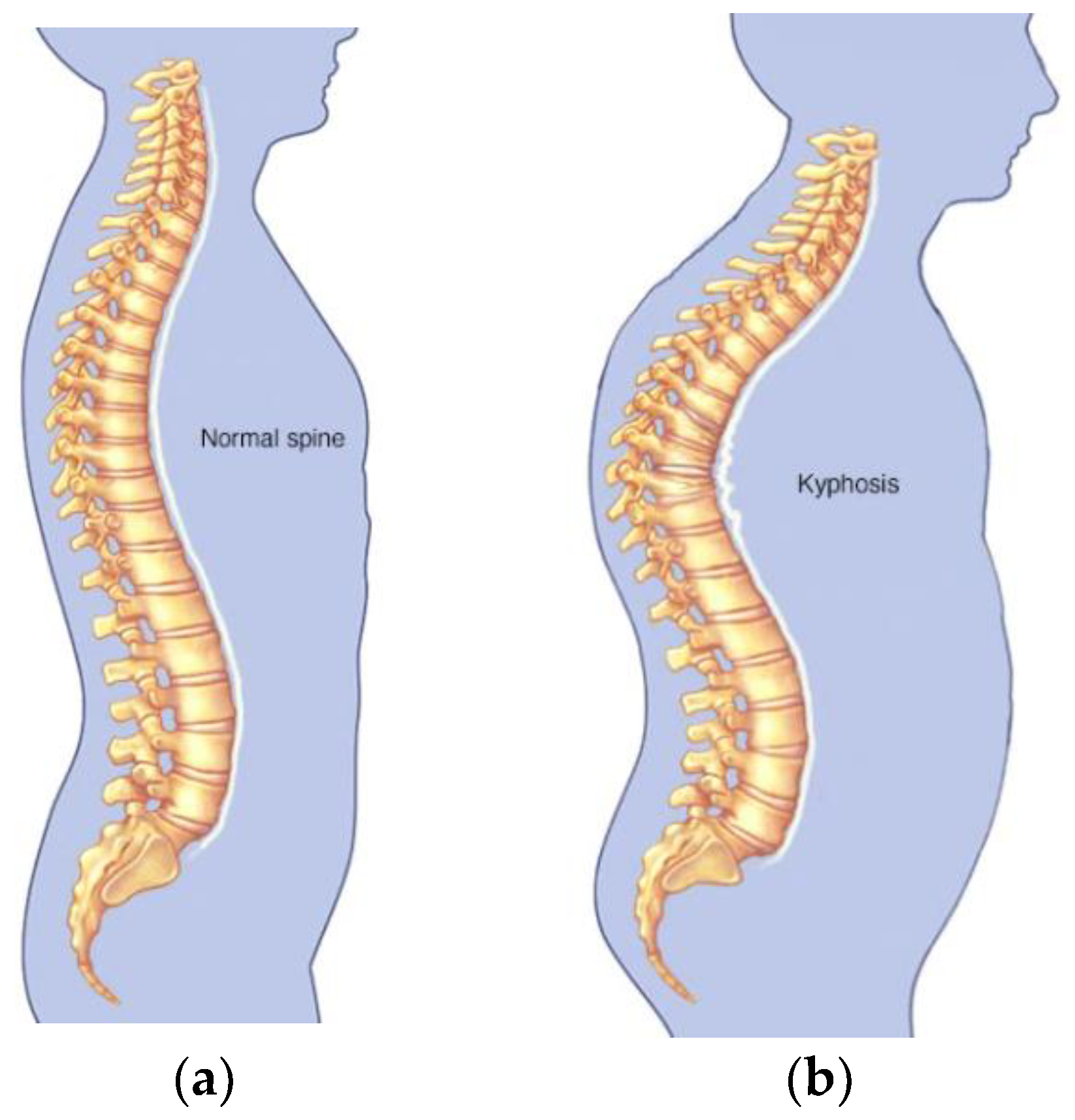
Kyphosis is an exaggerated, forward rounding of the back and which can occur at any age as shown in Figure 2b. Kyphosis can appear in infants or teenagers as a result to malformation of the spine of the spinal bones over time. Severe kyphosis can cause pain and disfiguring. Sometimes, the patient may experience back pain and stiffness in addition to an abnormally curved spine. Abnormal vertebrae can be caused by fractures (broken or crushed vertebrae), osteoporosis (bone-thinning disorder), disk degeneration (soft, circular disks act as cushions between spinal vertebrae), birth defects (spinal bones that don’t develop properly) etc. For further reading on kyphosis, refer to (https://www.mayoclinic.org/diseases-conditions/kyphosis/symptoms-causes/syc-20374205). More importantly, detecting kyphosis disease at the early stage in children will prevent abnormal spinal vertebrae problems.

Therefore, in this current research, based on a biomedical dataset, we apply Random Forest (RF), Support Vector Machines (SVM), and Artificial Neural Network (ANN) algorithms to build models to predict the absence or presence of a kyphosis disease based on a historical healthcare and personal records of a kyphosis disease patients after they have gone through surgery. The results of the models were then evaluated and compared.

The importance of this current research is to present to the biomedical community how machine learning algorithms have been applied to classify and predict kyphosis disease based on a biomedical data.

2. Materials and Methods

This section presents the dataset used, the preprocessing of the data and the machine learning algorithms, namely, Random Forest (RF), Support Vector Machines, and the Artificial Neural Network. The preprocessing of the data and the implementations of the models were achieved by using the Python environment. We used Python 3 as the version in writing the codes, which was achieved through the Jupyter Notebook by installing the Anaconda software (version 3.6, manufactured by the Anaconda Inc., Austin, TX, USA) (https://www.anaconda.com/).

2.1. Data and Preprocessing

We obtained the kyphosis [19] dataset from (https://www.kaggle.com/abbasit/kyphosis-dataset). The data has 81 rows and 4 columns which represents records on patients who have had corrective spinal surgery. The dataset is in a comma separate value (csv) format. Due to the small sample size of the data, we used all the data representing 100% for the training.

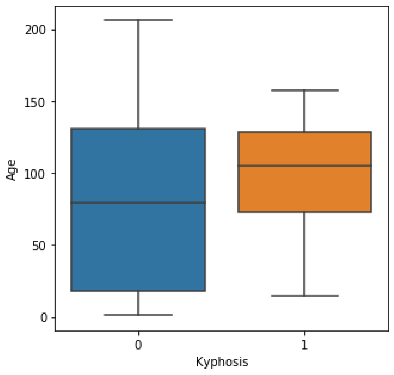
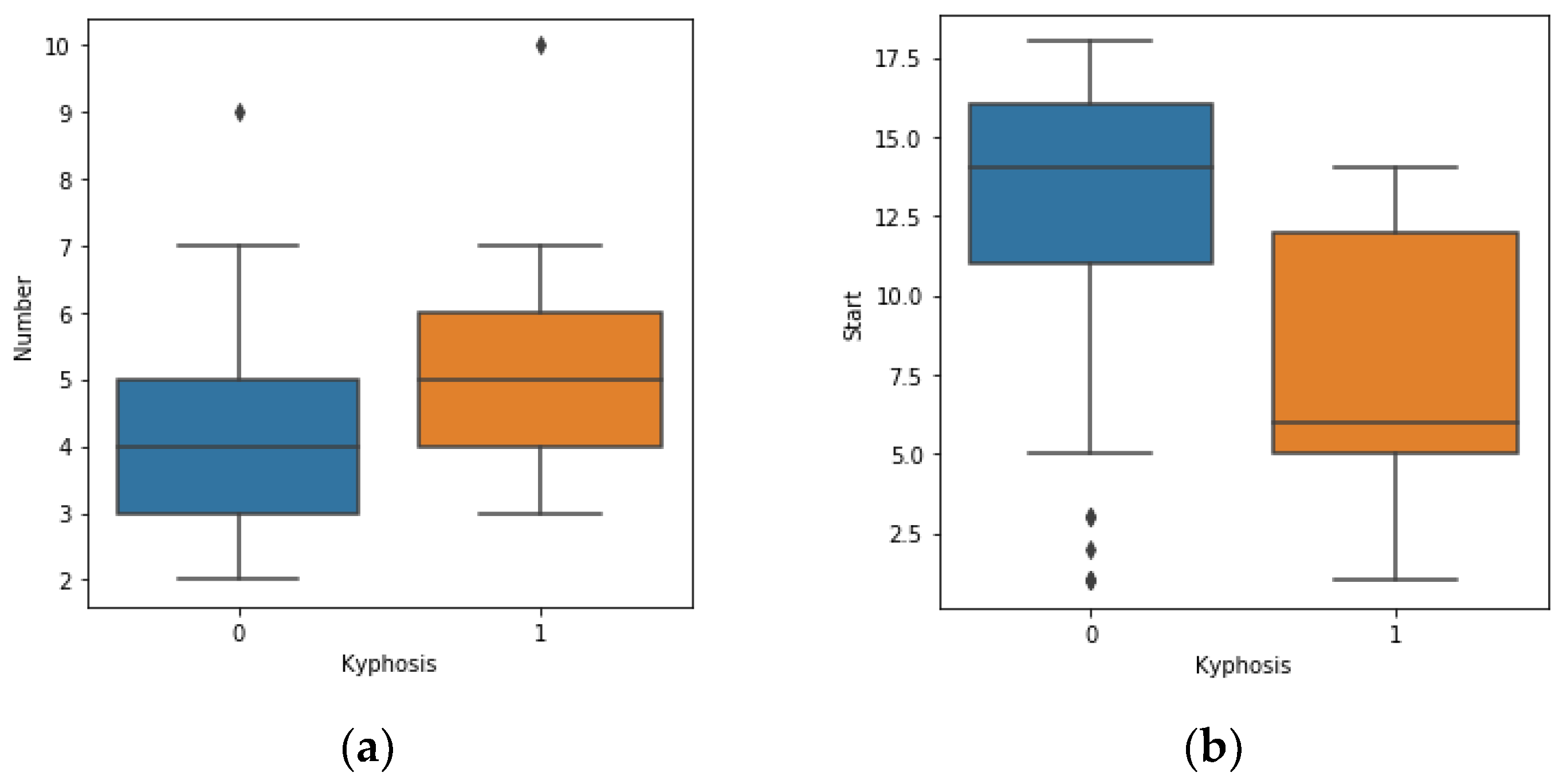
The features of the data represent 3 inputs and 1 output, where:

• Age: in months
• Number: the number of vertebrae involved
• Start: the number of the first (topmost) vertebrae operated on.

Output

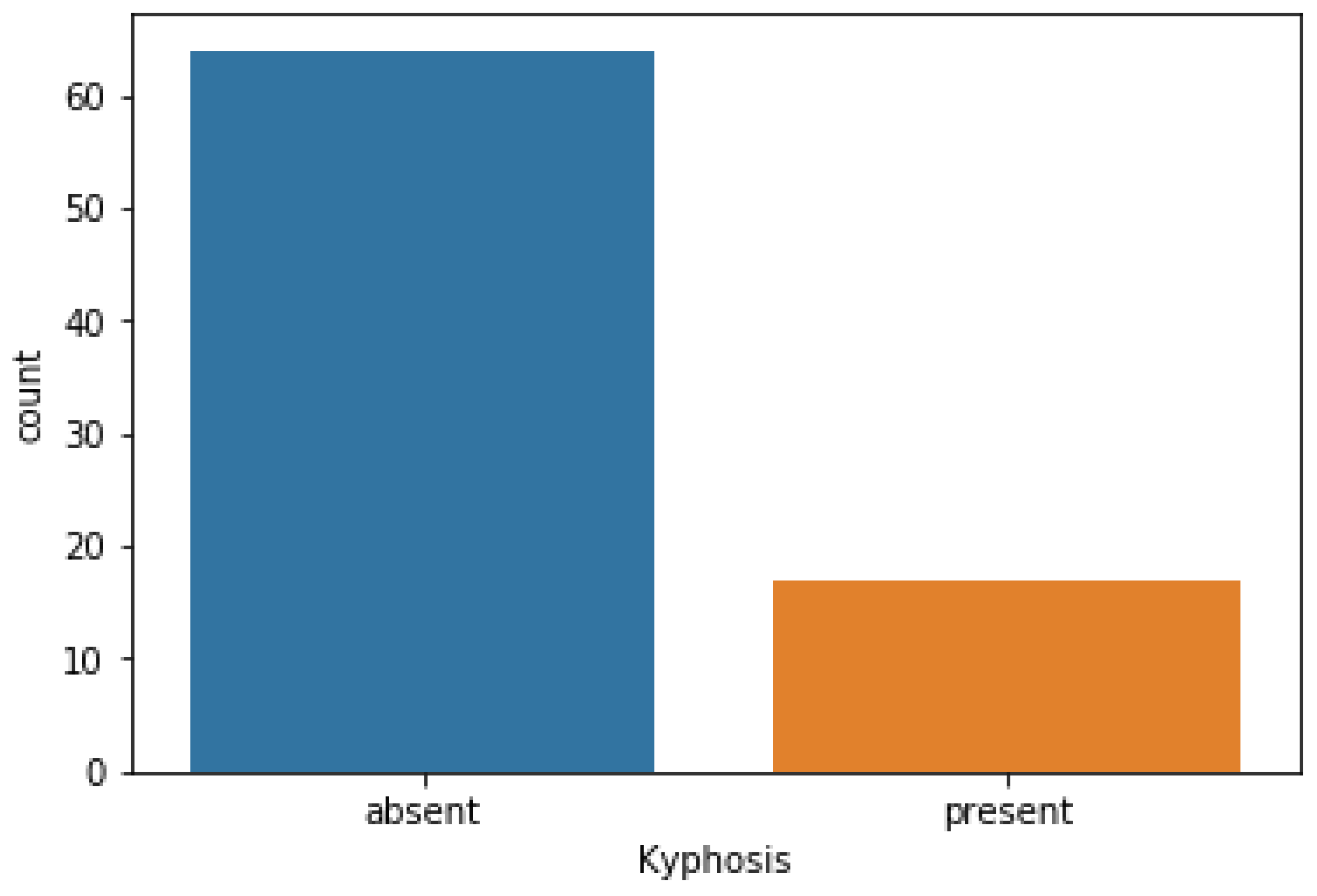
Kyphosis: a factor with levels absent or present indicating if a kyphosis (a type of deformation) was present after the operation or surgery.

In order to model the data, we processed the data in a format where the models can be trained.

We achieved the preprocessing of the data by using the Scikit-Learn library (https://scikit-learn.org/stable/index.html). Scikit-Learn helps to implement machine learning algorithms in Python, which provides simple and efficient tools for data mining and data analysis.

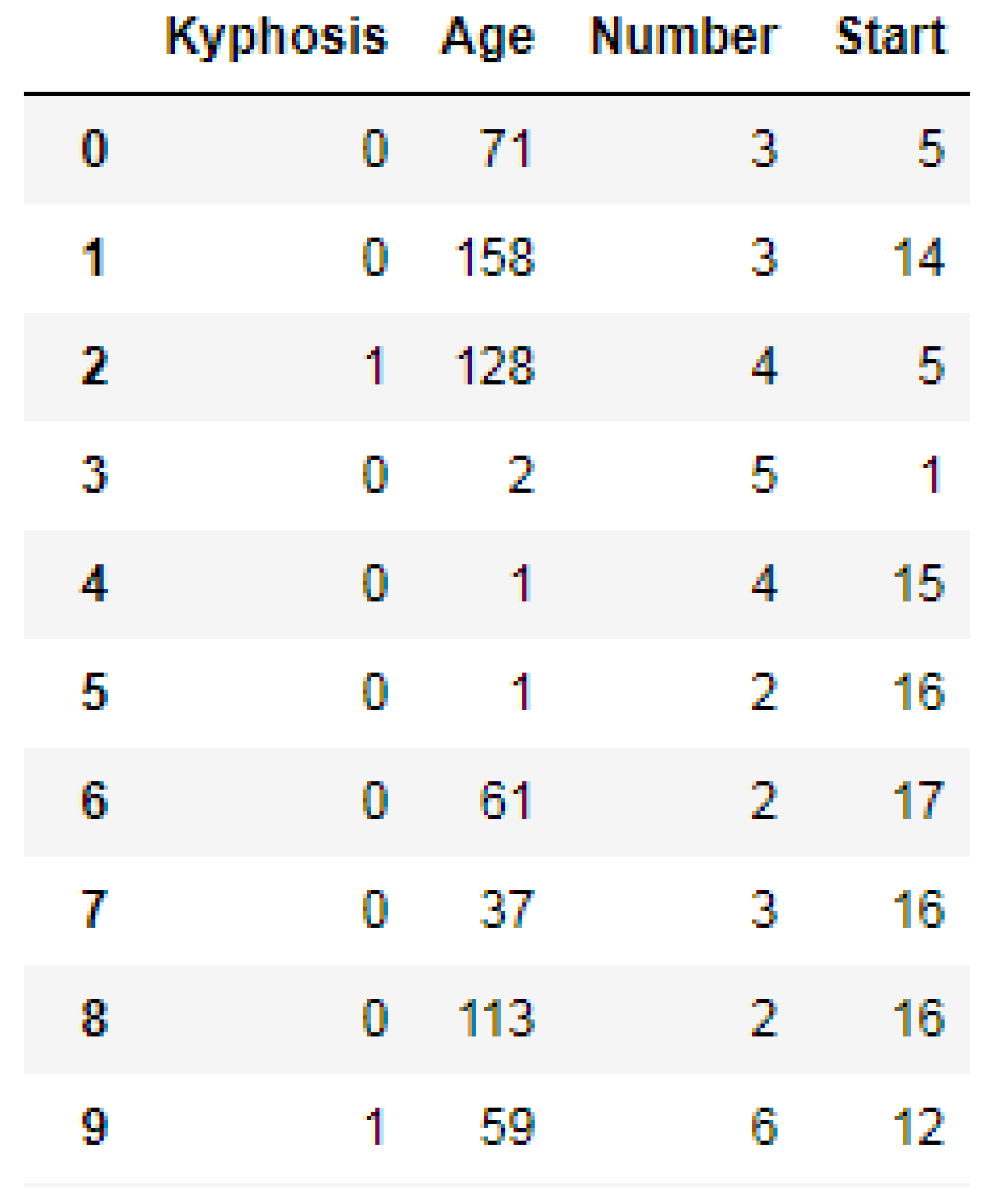
We used the Label Encoder function imported from the sklearn library to transform the Kyphosis column into zeros (0′s) and ones (1′s) as shown in Figure 3, where (1) represents presence of the disease and (0) represents absence of the disease. In order to obtain good performances by the models, we then standardized the data using the Standard Scaler function as a preprocessing tool which was imported from the sklearn library.

2.2. Logistic Regression

Logistic Regression (LR) is one of the fundamental and famous algorithms to solve classification problems. LR is used to obtain odds ratio in the presence of more than one independent variable [20]. LR deals with outliers by using sigmoid function. Therefore, Logistic function is a sigmoid function, which takes any real value between 0 and 1 [21]. It is mathematically expressed as:

$$\sigma \left(t\right)=\frac{e^t}{e^t+1}=\frac{1}{1+e^{-t}}$$

(1)

Considering t as a linear function in a univariate regression model:

$$t={\beta }_0+{\beta }_{1}x$$

(2)

Therefore, the Logistic Regression is represented as:

$$p\left(x\right)=\frac{1}{1+e^{-\left({\beta }_0+{\beta }_{1}x\right)}}$$

(3)

2.3. Random Forest

Random Forest was proposed by Breiman [22] as an ensemble classifier or regression tree based on many decision trees. Each of the trees is based on a bootstrap sample from the original training dataset using a tree classification procedure. Bootstrapping is a metric or test that depends on random sampling with replacement. A random selection of the whole variable set is used as variables for splitting the tree nodes. After formation of the forest, a new object which needs to be classified is noted for classification by each of the trees in the forest. A vote is cast by each of the trees to indicate the tree’s decision about the group or class of the object. The group or class with the majority of the votes is chosen by the forest.

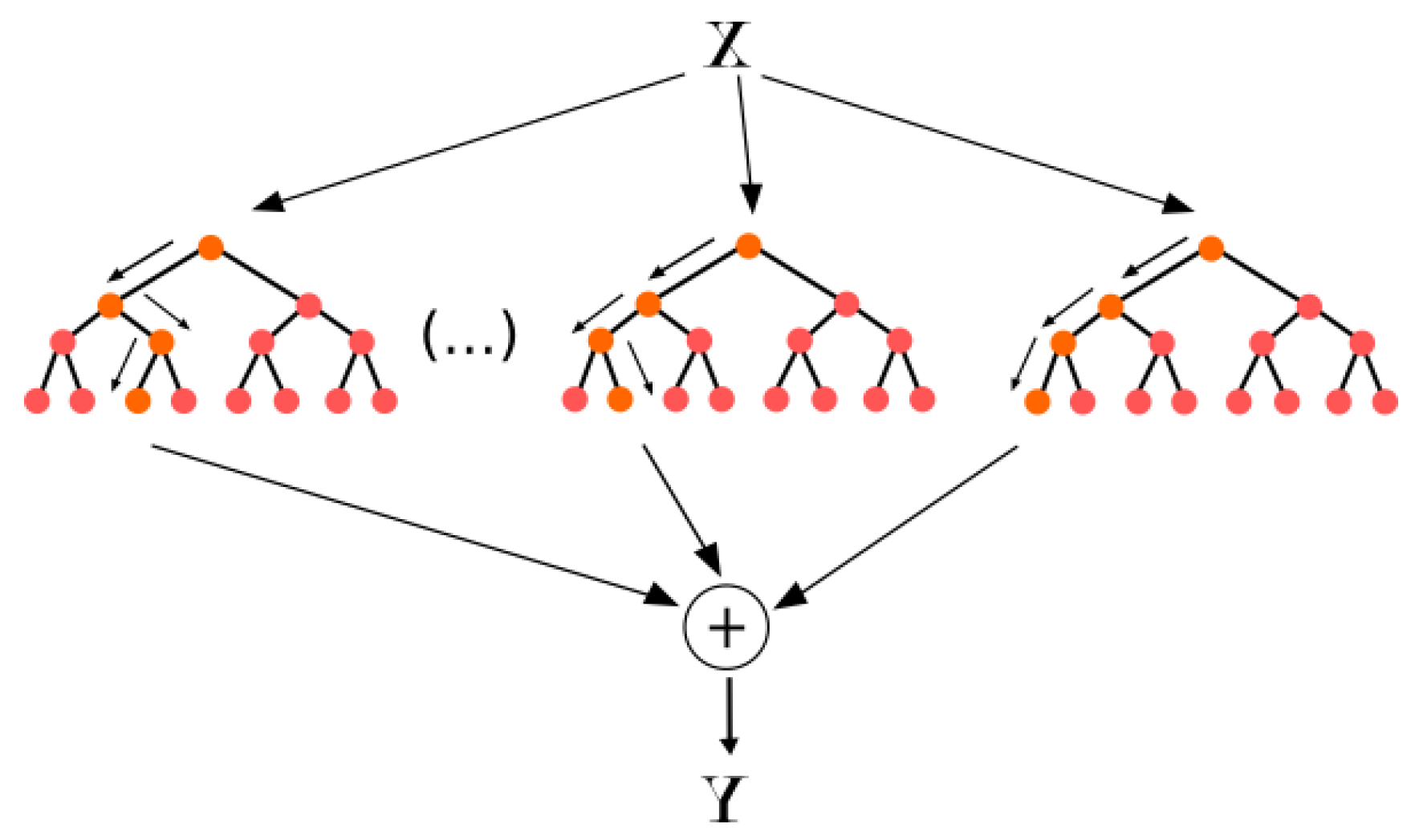
According to Neural Designer [23], Random Forest is one of the most famous algorithms used by data scientists. In Random Forest, each tree is influenced by the values of a random vector sampled independently as shown in Figure 4.

Random Forest algorithm follows as:

Select number of trees to grow (ntree)

➢

For i = 1 to ntree

• Randomly sample with replacement, same size as original dataset (bootstrap).
• Grow a tree.
• For every split of tree.
• Randomly select mtry predictors.
• Grow trees till stopping criteria is reached.
• Each tree then casts a vote for the most famous class, and the class with most votes wins.

➢

end

The formal definition of the random forest in our case is given as:

Assume training set (Kyphosis) of microarrays

$D=\{(X_1,y_1),\dots \dots .,\left(X_n,y_n\right)\}$, where D is the full dataset, is drawn from a random probability distribution $\left(X_i,y_i\right)\sim \left(X,\mathrm{Y}\right)$. The goal is to build a classifier which predicts y (target: kyphosis disease) from X (input features: Age, Number, Start) based on the dataset D.

Therefore, given ensemble of classifiers $h=\left\{h_1\left(X\right),\dots \dots h_{\mathrm{K}}\left(X\right)\right\}$, if each $h_{\mathrm{k}}\left(X\right)$ is a decision tree, then the ensemble is a random forest. We, therefore, define the parameters of the decision tree for classifier $h_{\mathrm{k}}\left(X\right)$ to be $\Theta {}_k=\left({\theta }_{k1},{\theta }_{k2}\dots \dots ,{\theta }_{kp}\right)$. The relationships between the classifiers and the parameters are sometimes given as $h_{\mathrm{k}}\left(X\right)=h\left(X|\Theta {}_k\right\}$. That is, decision tree k leads to a classifier $h_{\mathrm{k}}\left(X\right)=h(X|\Theta {}_k)$. The appearance of the features which are selected in the nodes of the $k^{th}$ occur at random, according to parameters $\Theta {}_k$, that are randomly chosen from a model variable $\Theta$.

The final classification $f\left(X\right)$ combines the classifiers $\left\{h_{\mathrm{k}}\left(X\right)\right\}$, each tree then casts a vote for the most famous class at input X, and the class with the most votes wins.

The RF model was achieved by importing the RF algorithm from the sklearn library. We further performed a grid search to help automate the selection of the best parameters to produce a model with the highest performance. The selected parameters for the grid search are as follows:

• n_estimators (100, 150, 200, 250, 300): this correspond to the number of trees in the forest.
• Criterion (gini, entropy): The criterion is the function used to measure the quality of the split. By default, gini is selected for the Gini impurity and entropy is for the information gain. They are in a string format.
• Bootstrap (true, false): The bootstrap is the random sampling with replacement. The bootstrap samples are used by default (bootstrap = True) whereas the default strategy for extra-trees is to use the whole dataset (bootstrap = False)

2.4. Support Vector Machine

Support Vector Machine theory is based on statistics which have a fundamental principle of estimating the optimal linear hyperplane in a feature space that maximally separates the two-mark groups or classes. SVM modeling geometrically finds an optimal hyperplane with the maximal interval to separate two groups or classes. The procedure for solving such a constraint problem is as follows [24,25,26,27]:

$$minimiz{e}_{w,b}\frac{1}{2}{\left|\left|w\right|\right|}^2$$

(4)

Subject to:

$y_i\left(w^T{x}_i+b\right)\ge 1,i=1,2,3,\dots .,n$, x = the feature vectors or the input pattern, w = the direction of the optimal hyperplane, b = bias

To make rooms for errors, the optimization problem currently becomes:

$$mi{n}_{w,b}\frac{1}{2}{\left|\left|w\right|\right|}^2+C{\displaystyle \sum }_{i=1}^n{\epsilon }_i$$

(5)

Subject to:

$$y_i\left(w^T{x}_i+b\right)\ge 1-{\epsilon }_i,i=1,2,3,\dots .,n$$

$${\epsilon }_i\ge 0,i=1,2,3,\dots .,n$$

The Lagrange multiplier method assists us to obtain the two formulas, that is expressed in terms of the variable α_i:

$$maximiz{e}_a{\displaystyle \sum }_{i=1}^n{\alpha }_i-\frac{1}{2}{\displaystyle \sum }_{i=1}^n{\displaystyle \sum }_{j=1}^n{\alpha }_i{\alpha }_j{y}_i{y}_j{x}_i^T{x}_j$$

(6)

Subject to:

$${{\displaystyle \sum }}_{i=1}^n{\alpha }_i{y}_i=1=0,0<\alpha <C$$

For all i = 1, 2, 3…., n

The linear classifier based on a linear discriminant function is then given as:

$$f\left(x\right)={\displaystyle \sum }_{i=1}^n{\alpha }_i{x}_i^{T}x+b$$

(7)

A non-linear classifier sometimes assists in providing better accuracy in many applications. A fragile way of making a non-linear classifier out of linear classifier is by mapping out data from the input space X to a feature space F based on a non-linear function $\varnothing :X\to F$. Using kernel function, in the space F, the optimization assumes the following:

$$maximiz{e}_a{\displaystyle \sum }_{i=1}^n{\alpha }_i-\frac{1}{2}{\displaystyle \sum }_{i=1}^n{\displaystyle \sum }_{j=1}^n{\alpha }_i{\alpha }_j{y}_i{y}_{j}k\left(x_i,x_j\right)$$

(8)

Subject to:

$${{\displaystyle \sum }}_{i=1}^n{y}_i{\alpha }_i=0,0<\alpha <C$$

For all i = 1, 2, 3…., n

The classifier $K\left(x,x^{\prime }\right)={\left(x.x^{\prime }\right)}^d$ is given as a SVM-Polynomial, where, if d is large, the kernel still requires n multiplications to compute. So, given

$$K\left(x,x^{\prime }\right)={\left(x.x^{\prime }\right)}^2={\left(\left(x_1,x_2\right).\left(x_1^{\prime },x_2^{\prime }\right)\right)}^2$$

(9)

The RBF classifier is given as

$$K\left(x,x^{\prime }\right)=\exp (-\gamma {\left|\left|x-x^{\prime }\right|\right|}^2$$

(10)

In this current research paper, we implemented (7), (9) and (10) as the SVM kernels which represent Linear, Polynomial and Radial Basis Function (RBF) respectively. The cost function (C) presents the measure of how wrong a model is in terms of its ability to estimate the relationship between x and y as seen from (11). The cost parameter was optimized by grid search in the training dataset. Given a Hypothesis -> H0 (x) = β0 + β1x, then the cost function (C) is represented as:

$$C=\frac{1}{2N}{\displaystyle \sum }_{i=1}^N\left(H_0\left(x\right)-y^{\left(i\right)}\right)$$

(11)

where N is the number of observations.

In developing the SVM classifiers, the values of the cost function used were (0.1, 1, 10, 100).

2.5. Artificial Neural Network

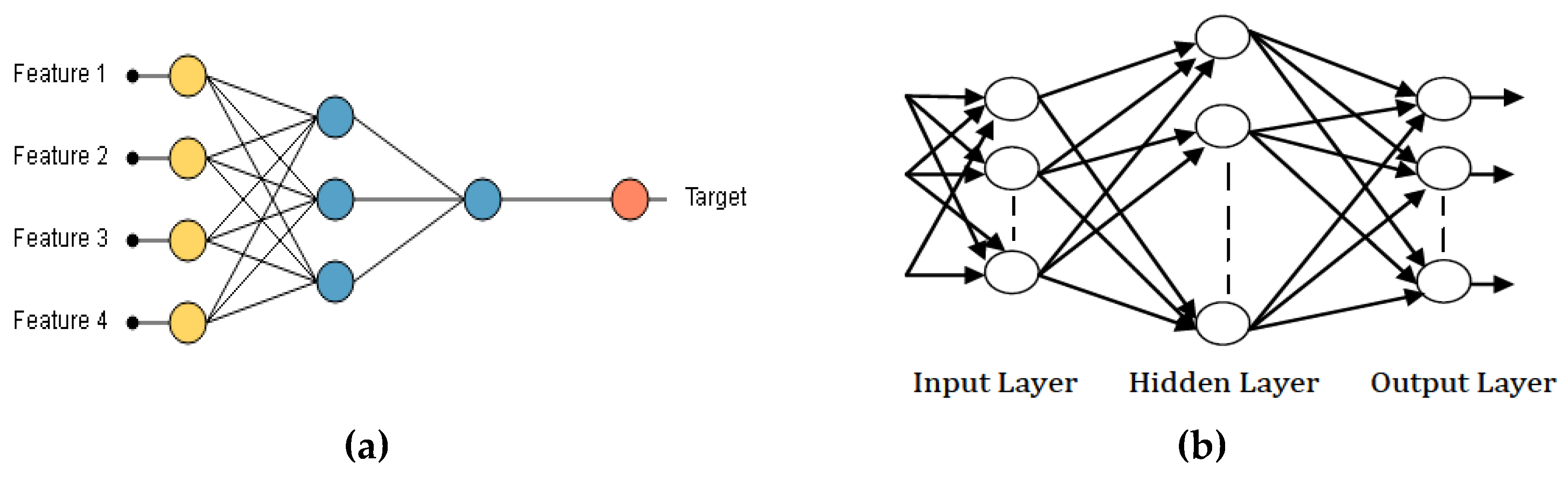
Artificial Neural Network is a computational model which depends on the neural structure of the brain. The outcome from the neural network is dependent on the features or inputs (Figure 5a) provided to it and the various parameters in the neural network. From Figure 5a, Feature 1, Feature 2, Feature 3, and Feature 4 represent the input samples while the target represents the output sample. In this current work, we designed a three-layered ANN [17], which includes input layer, Hidden Layer, and Output Layer as shown in Figure 5b.

In order to build neural networks, the following properties must be taken into consideration [28]:

• A set of inputs (1, …., n) (i).
• A set of outputs (1, …, m).
• Number of Hidden Layers.
• Number of neurons in each Hidden Layer.
• Bias for each neuron in the Hidden Layer (s) and Output Layer $\left(b_k\right)$.
• Weights of the bias in the Hidden Layer (s) and Output Layer $\left(v_k\right)$.
• Weights connecting neurons (w).

Therefore, the mathematical relation between these properties is given as:

$$\left({\displaystyle \sum }_m^n{i}_m{w}_m\right)+b_k{v}_k$$

(12)

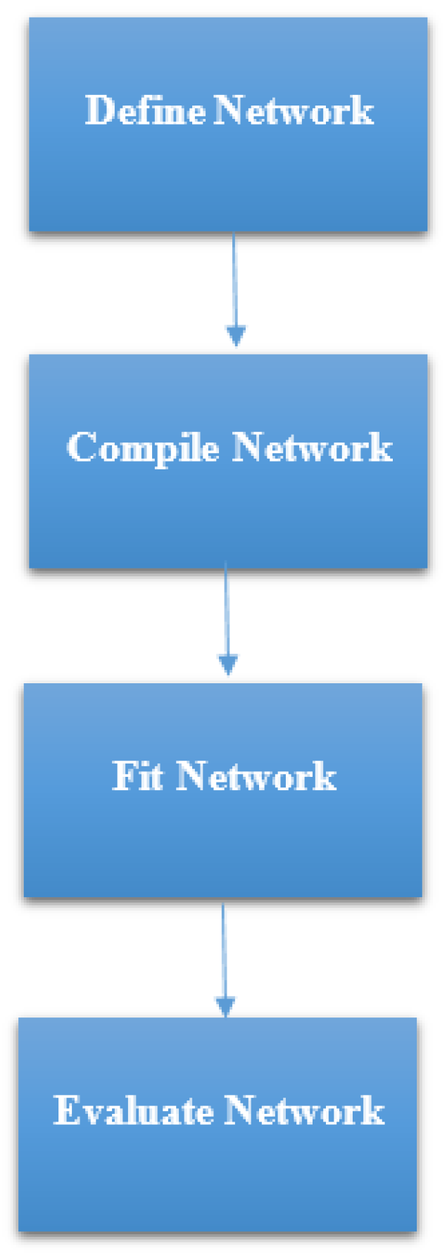
The implementation of the ANN model was achieved by using Keras (https://keras.io/). Keras is high-level neural networks Application Programming Interface (API) which was written in Python. It was built with a focus on enabling fast experimentation. The steps that were followed in developing the ANN model in this study, as summarized in Figure 6 were:

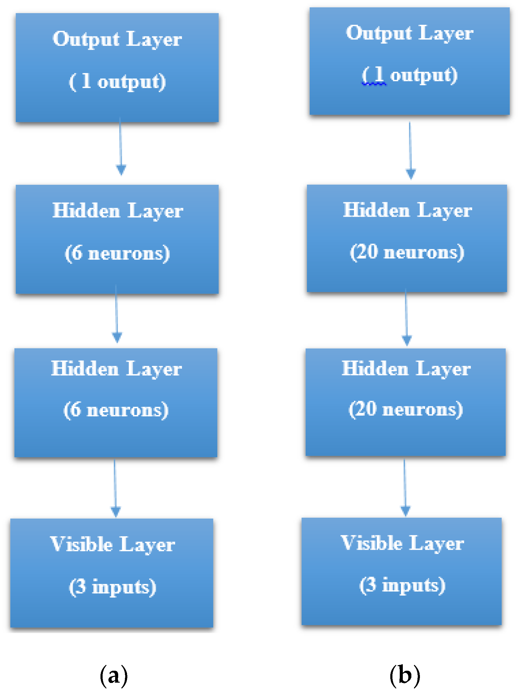
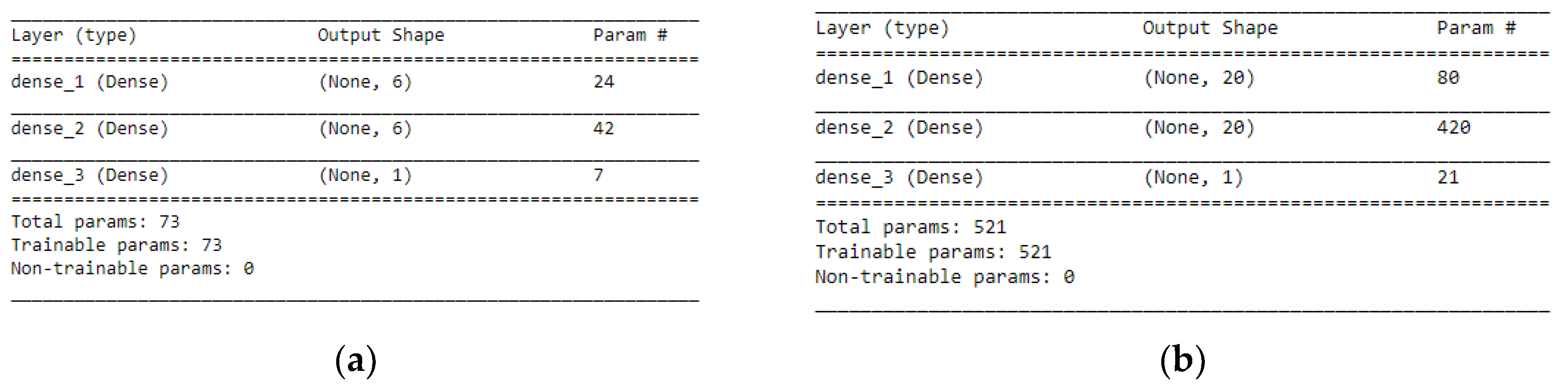
• STEP 1: Defining the network—We defined the model as a sequence of layers by using the sequential class in Keras. The sequential class serves as the container for the subsequent layers. In this current work, we built two architectures, which were, 3-6-6-1 network and 3-20-20-1 network as shown in Figure 7a, b respectively. Both the Hidden Layers were activated using the Rectified Linear Unit function (ReLu). The Output Layer was activated by using the sigmoid function, which is better when dealing with binary classification. The activation functions transform a summed signal from each neuron in a layer by extracting and adding to the sequential as a layer-like object. This was achieved by using the Activation class in Keras. In total, we observed a trainable parameter of 73 for the 3-6-6-1 network as shown in Figure 8a, and in the 3-20-20-1 network, we observed trainable parameters of 521 as shown in Figure 8b.
• STEP 2: Compile the network—After defining the network, we then compiled it. This step is efficient since it transforms the simple sequence of layers that we have defined into highly efficient series of matrix in a format intended to be executed on the CPU. In this work, we achieved the compiling of our network by using the compile class in Keras which has optimization algorithm, loss function, and metrics as parameters. We compared both Adam [29] and RMSprop (Root Mean Square probability) as the optimization algorithms and binary_crossentropy as the loss function.
• STEP 3: Fit the Network—The compiled model is then fit, means adapting the model weights in response to the training dataset. In this step, we specified the training dataset with matrix of input patterns, X, and array of the matching output patterns, y. Here, we compared a batch size of 25 and 32. We also compared epochs of 100 and 500.
• STEP 4: Evaluate the Network—In this current work, the ANN model was evaluated using K-Fold Cross-Validation, by which much detailed is given in Section 2.6.

2.6. Evaluation of the Models

According to k-Fold Cross-Validating Neural Networks [30], it can be useful to benefit from K-Fold cross-validation when dealing with a small sample size, in order to maximize the ability to evaluate the performance of the model. In addition, as stated by Cross-Validation: Evaluating Estimator Performance [31], it would be a methodological mistake to learn the parameters of a prediction function and then test it on the same data. They further stated that the best parameters can be achieved by using grid search method.

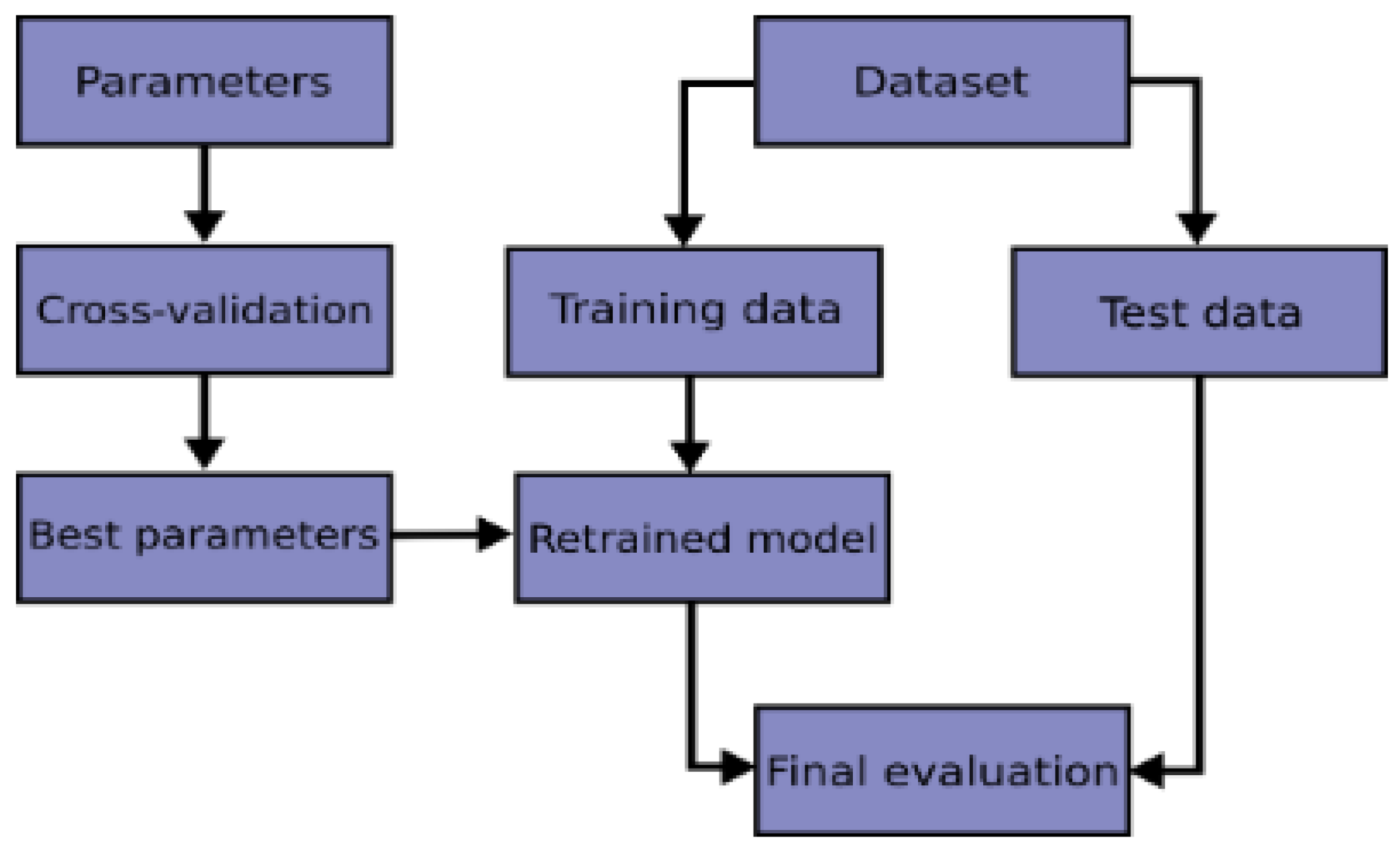
Therefore, in this current work, we performed K-Fold cross-validation to evaluate our models and then used grid search technique to choose the best parameters that helped to produce high performance. The flowchart of a typical cross-validation workflow can be seen from Figure 9.

The process of the K-Fold cross-validation is explained as:

• Divide the data into K folds.
• Out of the K folds, K-1 sets are used for training whereas the remaining set is used for testing.
• The model is then trained and tested K times, each time a new set is used as testing whereas the remaining sets are used for training.
• Lastly, the result of the K-Fold cross-validation is the average of the results obtained on each set.

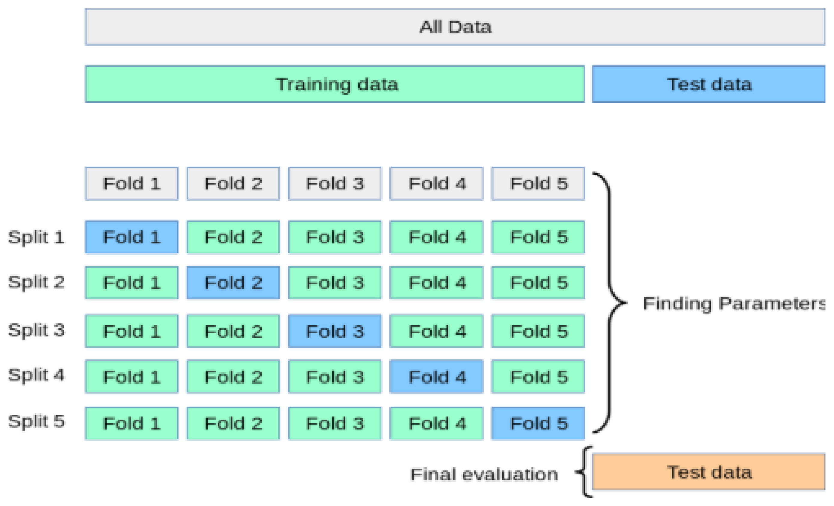
The process of the K-Fold cross-validation can be illustrated as shown in Figure 10.

The only problem was how to use the K-Fold cross-validation from the Sci-Kit Learn library on the ANN models. The problem was that the ANN algorithm is not part of the Sci-Kit Learn learning algorithm, which produced error. We then solved this problem by wrapping the neural networks with the KerasClassifier class [30], which helped us to use the Sci-Kit Learn. This method rendered the neural networks to behave as any other Sci-Kit Learn learning algorithm (Random forest, SVM). In this current work, we performed both 5- and 10-Fold Cross-Validation based on empirical evidence that 5- or 10-Fold Cross Validation should be preferred [31].

3. Results

This section presents the results of the research work after performing an exploratory analysis on the kyphosis dataset, modeling the RF, SVM-linear, SVM-RBF, SVM-Poly and the ANN algorithms using 5- and 10-Fold Cross-Validations. We present the results of the machine learning (ML) models after performing grid search with cross-validation. We have further compared our ML results with Logistic Regression as a baseline model to evaluate the performance of our models.

3.1. Exploratory Analysis of the Kyphosis Data

Exploratory analysis showed that there were 79% of patients reported showing absence of Kyphosis while 21% of patients reported showing presence of the disease based on Figure 11. From Figure 12a, some correlation between kyphosis and the number (the number of vertebrae involved) representing 0.36 could be seen. The patterns of the kyphosis disease being absence or presence can be seen from Figure 12b based on the features of the patients. It can be seen that separating the two classes would be an easy task based on the patterns identified. We further performed outlier detection by using a boxplot as shown in Figure 13 and Figure 14a,b. We detected some outliers in the data as shown in Figure 14a,b. We then rectified this problem by normalizing the dataset.

3.2. The Logistic Regression (LR) Model Outcomes Based on K-Fold Cross-Validation

After training the Logistic Regression (LR) model, by performing 5-Fold Cross-Validation,

Table 1. Accuracies achieved by performing 5-Fold Cross-Validation on the Logistic Regression (LR) model.

K-Fold	Accuracy
1	0.7647
2	0.7059
3	0.9375
4	0.8125
5	0.8667
Mean: 81.75%	Std: 0.0801

shows the accuracies achieved by the various K-Folds. The highest accuracy was detected at Fold 3, which was 0.9375 as visualized in Figure 15. The LR model achieved a mean accuracy of 81.75% and a standard deviation of 0.0801 based on the 5-Fold Cross-Validation. After further training the LR model, by performing 10-Fold Cross-Validation,

Table 2. Accuracies achieved by performing 10-Fold Cross-Validation on the LR model.

K-Fold	Accuracy
1	0.8889
2	0.5556
3	0.5556
4	0.8889
5	0.8750
6	1.0000
7	0.7500
8	0.7143
9	0.8571
10	0.8571
Mean: 79.42%	Std: 0.1403

shows the accuracies by the various K-Folds. The highest accuracy was detected at Fold 6, which was 1.0000, as visualized in Figure 16. The RF model then achieved a mean accuracy of 79.42% and a standard deviation of 0.1403 based on the 10-Fold Cross-Validation.

3.3. The Random Forest Model Outcomes Based on K-Fold Cross-Validation and Grid Search

After training the RF model, by performing 5-Fold Cross-Validation,

Table 3. Accuracies achieved by performing 5-Fold Cross-Validation on the RF model.

K-Fold	Accuracy
1	0.7647
2	0.8750
3	0.8235
4	0.6875
5	0.8000
Mean: 79.01%	Std: 0.0626

shows the accuracies achieved by the various K-Folds. The highest accuracy was detected at Fold 2, which was 0.8750 as visualized in Figure 17. The RF model achieved a mean accuracy of 79.01% and a standard deviation of 0.0626 based on the 5-Fold Cross-Validation. Based on a grid search with 5-Fold CV, the best parameters were selected at {“bootstrap”: True, “criterion”: “entropy”, “n_estimators”: 100}, which achieved an accuracy of 80.25% as seen from Figure 18.

After further training the RF model, by performing 10-Fold Cross-Validation,

Table 4. Accuracies achieved by performing 10-Fold Cross-Validation on the RF model.

K-Fold	Accuracy
1	0.8889
2	0.6667
3	0.8889
4	0.7778
5	0.6250
6	0.7500
7	0.7500
8	0.7143
9	0.8571
10	0.8571
Mean: 77.76%	Std: 0.0886

shows the accuracies by the various K-Folds. The highest accuracy was detected at Fold 1 and Fold 3, by which both Folds achieved 0.8889 as visualized in Figure 19. The RF model then achieved a mean accuracy of 77.76% and a standard deviation of 0.0886 based on the 10-Fold Cross-Validation. Based on a grid search with the 10-Fold CV, the best parameters were selected at {“bootstrap”: True, “criterion”: “gini”, “n_estimators”: 100}, which achieved an accuracy of 80.25% as seen from Figure 20.

3.4. The SVM-Linear Model Outcomes Based on K-Fold Cross-Validation and Grid Search

After training the SVM-Linear model, by performing 5-Fold Cross-Validation,

Table 5. Accuracies achieved by performing 5-Fold Cross-Validation on the SVM-Linear model.

K-Fold	Accuracy
1	0.7647
2	0.7059
3	0.8125
4	0.8125
5	0.8667
Mean: 79.25%	Std: 0.0540

shows the accuracies by the various K-Folds. The highest accuracy was detected at Fold 5, which was 0.8667 as visualized in Figure 21. The SVM-Linear model achieved a mean accuracy of 79.25% and a standard deviation of 0.0540 based on the 5-Fold Cross-Validation. Based on grid search with 5-Fold CV, the best parameters were selected at {“C”: 1, “gamma”: 1, “kernel”: “linear”}, which achieved an accuracy of 79.01% as seen from Figure 22.

After further training the SVM-Linear model, by performing 10-Fold Cross-Validation,

Table 6. Accuracies achieved by performing 10-Fold Cross-Validation on the SVM-Linear model.

K-Fold	Accuracy
1	0.7776
2	0.6667
3	0.5556
4	0.7776
5	0.8750
6	0.7500
7	0.7500
8	0.7143
9	1.0000
10	0.8571
Mean: 77.24%	Std: 0.1150

shows the accuracies by the various K-Folds. The highest accuracy was detected at Fold 9, which achieved 1.0000 as visualized in Figure 23. The SVM-Linear model then achieved a mean accuracy of 77.24% and a standard deviation of 0.1150 based on the 10-Fold Cross-Validation. Based on a grid search with the 10-Fold CV, the best parameters were selected at {“C”: 0.1, “gamma”: 1, “kernel”: “linear”}, which achieved an accuracy of 77.76% as seen from Figure 24.

3.5. The SVM-RBF Model Outcomes Based on K-Fold Cross-Validation and Grid Search

After training the SVM-RBF model, by performing 5-Fold Cross-Validation,

Table 7. Accuracies achieved by performing 5-Fold Cross-Validation on the SVM-RBF model.

K-Fold	Accuracy
1	0.8235
2	0.8826
3	0.8750
4	0.7500
5	0.8000
Mean: 82.62%	Std: 0.0490

shows the accuracies by the various K-Folds. The highest accuracy was detected at Fold 2, which was 0.8826 as visualized in Figure 25. The SVM-RBF model achieved a mean accuracy of 82.62% and a standard deviation of 0.0490 based on the 5-Fold Cross-Validation. Based on a grid search with 5-Fold CV, the best parameters were selected at {“C”: 1, “gamma”: 1, “kernel”: “rbf”}, which achieved an accuracy of 82.72% as seen from Figure 26.

After further training the SVM-RBF model, by performing 10-Fold Cross-Validation,

Table 8. Accuracies achieved by performing 5-Fold Cross-Validation on the SVM-RBF model.

K-Fold	Accuracy
1	0.8889
2	0.7776
3	0.8889
4	0.7776
5	0.6250
6	0.7500
7	0.7500
8	0.7143
9	0.8571
10	0.8571
Mean: 78.87%	Std: 0.0806

shows the accuracies by the various K-Folds. The highest accuracy was detected at Fold 1 and Fold 3, by which both Folds achieved 0.8889 as visualized in Figure 27. The SVM-RBF model then achieved a mean accuracy of 78.87% and a standard deviation of 0.0806 based on the 10-Fold Cross-Validation. Based on a grid search with the 10-Fold CV, the best parameters were selected at {“C”: 10, “gamma”: 0.1, “kernel”: “rbf”}, which achieved an accuracy of 85.19% as seen from Figure 28.

3.6. The SVM-Polynomial Model Outcomes Based on K-Fold Cross-Validation and Grid Search

After training the SVM-Polynomial model, by performing 5-Fold Cross-Validation,

Table 9. Accuracies achieved by performing 5-Fold Cross-Validation on the SVM-Polynomial model.

K-Fold	Accuracy
1	0.7647
2	0.7647
3	0.8125
4	0.8125
5	0.6667
Mean: 76.42%	Std: 0.0533

shows the accuracies by the various K-Folds. The highest accuracy was detected at Fold 1 and Fold 3, by which both Folds achieved 0.8125 as visualized in Figure 29. The SVM-Polynomial model achieved a mean accuracy of 76.42% and a standard deviation of 0.0533 based on the 5-Fold Cross-Validation. Based on grid search with 5-Fold CV, the best parameters were selected at {“C”: 0.1, “gamma”: 0.1, “kernel”: “poly”}, which achieved an accuracy of 79.01% as seen from Figure 30.

After further training the SVM-Poly model, by performing 10-Fold Cross-Validation,

Table 10. Accuracies achieved by performing 5-Fold Cross-Validation on the SVM-Poly model.

K-Fold	Accuracy
1	0.7778
2	0.6667
3	0.7778
4	0.7778
5	0.6250
6	0.7500
7	0.7500
8	0.8571
9	0.8571
10	0.8571
Mean: 76.96%	Std: 0.0745

shows the accuracies by the various K-Folds. The highest accuracy was detected at Fold 8, Fold 9, and Fold 10, by which all the three Folds achieved 0.8571 as visualized in Figure 31. The SVM-Poly model then achieved a mean accuracy of 76.96% and a standard deviation of 0.0745 based on the 10-Fold Cross-Validation. Based on a grid search with the 10-Fold CV, the best parameters were selected at {“C”: 0.1, “gamma”: 0.1, “kernel”: “poly”}, which achieved an accuracy of 79.01% as seen from Figure 32.

3.7. The ANN (3-6-6-1) Model Outcomes Based on K-Fold Cross-Validation and Grid Search

After training the ANN (3-6-6-1) model, by performing 5-Fold Cross-Validation,

Table 11. Accuracies achieved by performing 5-Fold Cross-Validation on the ANN (3-6-6-1) model.

K-Fold	Accuracy
1	0.7059
2	0.8750
3	0.8125
4	0.8125
5	0.7500
Mean: 79.12%	Std: 0.0581

shows the accuracies by the various K-Folds. The highest accuracy was detected at Fold 2, which achieved 0.8750 as visualized in Figure 33. The ANN (3-6-6-1) model achieved a mean accuracy of 79.12% and a standard deviation of 0.0581 based on the 5-Fold Cross-Validation. Based on a grid search with 5-Fold CV, the best parameters were selected at {“batch_size”: 25, “epochs”: 500, “optimizer”: “adam”}, which achieved an accuracy of 85.19% as seen from Figure 34.

After further training the ANN (3-6-6-1) model, by performing 10-Fold Cross-Validation,

Table 12. Accuracies achieved by performing 10-Fold Cross-Validation on the ANN (3-6-6-1) model.

K-Fold	Accuracy
1	0.7778
2	0.6250
3	0.7500
4	1.0000
5	0.8750
6	0.7500
7	0.7500
8	0.8750
9	0.7500
10	0.7500
Mean: 79.03%	Std: 0.0969

shows the accuracies by the various K-Folds. The highest accuracy was detected at Fold 4, which achieved 1.0000 as visualized in Figure 35. The ANN (3-6-6-1) model then achieved a mean accuracy of 79.03% and a standard deviation of 0.0969 based on the 10-Fold Cross-Validation. Based on a grid search with the 10-Fold CV, the best parameters were selected at {“batch_size”: 32, “epochs”: 500, “optimizer”: “rmsprop”}, which achieved an accuracy of 86.42% as seen from Figure 36.

3.8. The ANN (3-20-20-1) Model Outcomes Based on K-Fold Cross-Validation and Grid Search

After training the ANN (3-20-20-1) model, by performing 5-Fold Cross-Validation,

Table 13. Accuracies achieved by performing 5-Fold Cross-Validation on the ANN (3-20-20-1) model.

K-Fold	Accuracy
1	0.7059
2	0.8750
3	0.8125
4	0.8125
5	0.7500
Mean: 79.12%	Std: 0.0581

shows the accuracies by the various K-Folds. The highest accuracy was detected at Fold 2, which achieved 0.8750 as visualized in Figure 37. The ANN (3-20-20-1) model achieved a mean accuracy of 79.12% and a standard deviation of 0.0581 based on the 5-Fold Cross-Validation. Based on a grid search with 5-Fold CV, the best parameters were selected at {“batch_size”: 25, “epochs”: 100, “optimizer”: “adam”}, which achieved an accuracy of 83.95% as seen from Figure 38.

After further training the ANN (3-20-20-1) model, by performing 10-Fold Cross-Validation,

Table 14. Accuracies achieved by performing 10-Fold Cross-Validation on the ANN (3-20-20-1) model.

K-Fold	Accuracy
1	0.7778
2	0.6250
3	0.7500
4	1.0000
5	0.8750
6	0.7500
7	0.7500
8	0.8750
9	0.7500
10	0.7500
Mean: 79.03%	Std: 0.0969

shows the accuracies by the various K-Folds. The highest accuracy was detected at Fold 4, which achieved 1.0000 as visualized in Figure 39. The ANN (3-20-20-1) model then achieved a mean accuracy of 79.03% and a standard deviation of 0.0969 based on the 10-Fold Cross-Validation. Based on a grid search with the 10-Fold CV, the best parameters were selected at {“batch_size”: 25, “epochs”: 500, “optimizer”: “adam”}, which achieved an accuracy of 85.19% as seen from Figure 40.

4. Discussion

In previous works, other practitioners have compared and applied several machine learning algorithms to diagnose and predict diseases [7,9,10,11,12,13,14,15,16,17,32]. When it comes to a literature review on using machine learning algorithms in predicting other diseases, the work of Animesh et al. [12] has done a good job. In the work of Kavitha et al. [13], they modeled an ANN to detect heart disease using 13 inputs, 2 hidden nodes and 1 output. Also, the work of Noura [14] used ANN to predict heart disease, which achieved 88% accuracy. It was further stated that ANN is broadly used in medical diagnosis and healthcare systems as result to the predictive power it possesses as a model as confirmed by Animesh et al. [12]. The work of Mrudula et al. [15] compared SVM and ANN to predict heart disease, they stated that, ANN outperformed the SVM model to predict the disease.

Furthermore, the work of Tahmooresi et al. [2] compared several machine learning algorithms such as SVM, ANN, KNN, DT for breast cancer detection. They have performed an in-depth literature review on various machine learning algorithms for further reading. They concluded that SVM outperformed all the other models, which achieved an accuracy of 99.8% to detect the breast cancer disease. Also, the work of Ayeldeen et al. [16] compared several machine learning algorithms on a case-based retrieval approach of clinical breast cancer patients. They concluded that the RF model showed the maximum accuracy of 99%. The work of Kuo et al. [18] compared the performance of naïve-Bayesian, SVM, logistic regression, C4.5 decision tree, and random forest methods in predicting the medical costs of spinal fusion. They concluded that the random forest algorithm had the best predictive performance in comparison to the other techniques, achieving an accuracy of 84.30%, a sensitivity of 71.4%, a specificity of 92.2%, and an AUC of 0.904. ly. This predictive power of RF model can be noticed in this current research work in terms of accuracy as shown in

Table 15. The accuracies achieved by the machine learning (ML) models after performing grid search with 5-Fold Cross-Validation.

Model	Best Parameters	Accuracy (%)
RF	{‘bootstrap’: True, ‘criterion’: ‘entropy’, ‘n_estimators’: 100}	80.25
SVM-Linear	{‘C’: 1, ‘gamma’: 1,‘kernel’: ‘linear’},	79.01
SVM-RBF	{‘C’: 1, ‘gamma’: 1, ‘kernel’: ‘rbf’}	82.72
SVM-Poly	{‘C’:0.1, ‘gamma’:0.1, ‘kernel’: ‘poly’}	79.01
ANN (3-6-6-1)	{‘batch_size’: 25, ‘epochs’: 500, ‘optimizer’: ‘adam’}	85.19
ANN (3-20-20-1)	{‘batch_size’: 25, ‘epochs’: 100, ‘optimizer’: ‘adam’},	83.95

and

Table 16. The accuracies achieved by the ML models after performing grid search with 10-Fold Cross-Validation.

Model	Best Parameters	Accuracy (%)
RF	{‘bootstrap’: True, ‘criterion’: ‘gini’, ‘n_estimators’: 100	80.25
SVM-Linear	{‘C’:0.1, ‘gamma’:1, ‘kernel’: ‘linear’}	77.76
SVM-RBF	{‘C’: 10, ‘gamma’: 0.1, ‘kernel’: ‘rbf’}	85.19
SVM-Poly	{‘C’: 0.1, ‘gamma’: 0.1, ‘kernel’: ‘polyf’},	79.01
ANN (3-6-6-1)	{‘batch_size’: 32, ‘epochs’: 500, ‘optimizer’: ‘rmsprop’}	86.42
ANN (3-20-20-1)	{‘batch_size’: 25, ‘epochs’: 500, ‘optimizer’: ‘adam’},	85.19

.

And lastly, in the work of Abdullah et al. [8], they used machine learning techniques to predict spinal abnormalities based on KNN and RF models. They concluded that the KNN model which achieved an accuracy of 85.32% outperformed the RF model which had an accuracy of 79.57%.

Therefore, the purpose of this current research was to compare the performances of three most used and famous machine learning algorithms such as the RF, SVM, and ANN in the classification and prediction of kyphosis disease based on a biomedical dataset.

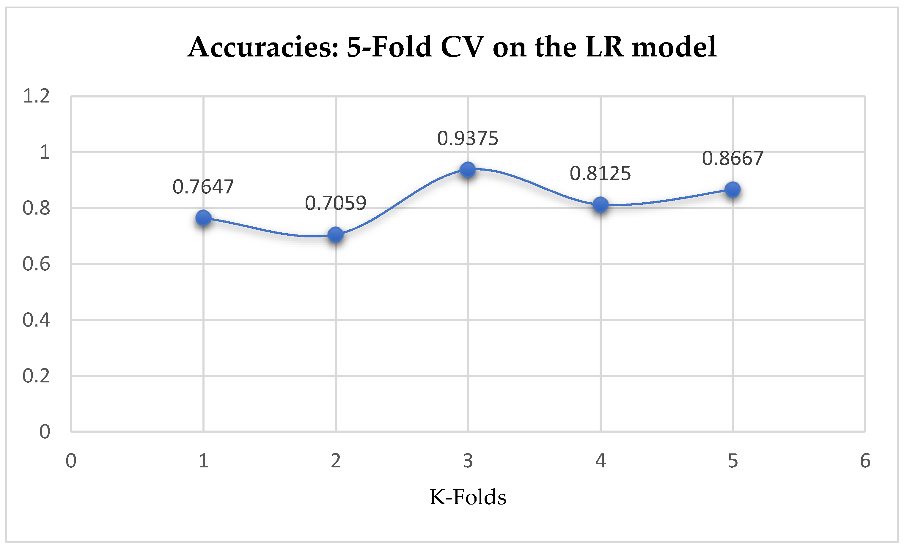
At first, we performed 5-Fold and 10-Fold Cross-Validations using Logistic Regression as a baseline model to compare with our ML models in terms of K-Fold CV without performing grid searching. The idea was based on the assumption concluded in the work of Christodoulou et al. [33] that they found no evidence of superior performance of machine learning over Logistic Regression when performing clinical prediction modeling. 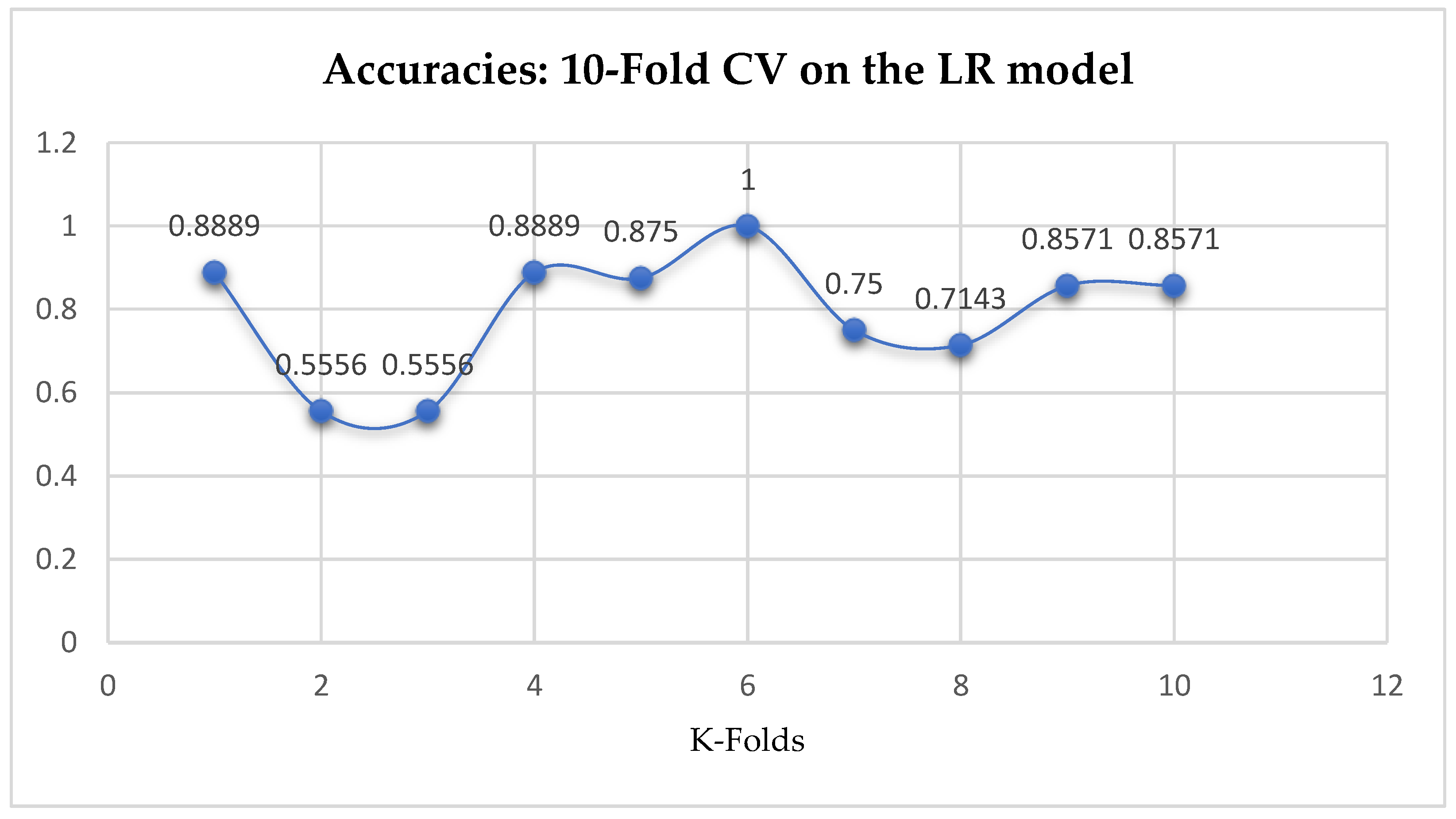We observed a mean accuracy of 81.75% as seen from Figure 15, based on the 5-Fold Cross-Validation after evaluating the LR model. After performing 10-Fold Cross-Validation, the LR model achieved a mean accuracy of 79.42% as seen from Figure 15.

Based on the ML models, we performed two categories of experiments, (1) K-Fold Cross-Validation without Grid Search, and (2) Grid Search with K-Fold Cross-Validation. In each of the experiments, we performed both 5-Fold and 10-Fold Cross-Validation. When dealing with K-Fold Cross-Validation, 5 or 10 Fold is mostly preferred [30].

In terms of the 5-Fold Cross-Validation, without Grid Searching, the RF model achieved a mean accuracy of 79.01%. By evaluating the RF model based on the K-Fold Cross-Validation, without grid searching, the baseline model, LR outperformed the RF model as seen from

Table 17. A Comparison of the accuracies achieved by the ML models and the baseline model (LR) after performing 5- and 10-Fold Cross-Validation without running grid search algorithm.

Model	5-Fold Cross-Validation (ACC%)	10-Fold Cross-Validation (ACC%)
LR	81.75	79.42
RF	79.01	77.76
SVM-Linear	79.25	77.24
SVM-RBF	82.62	78.87
SVM-Poly	76.42	76.96
ANN (3-6-6-1)	79.12	79.03
ANN (3-20-20-1)	79.12	79.03

.

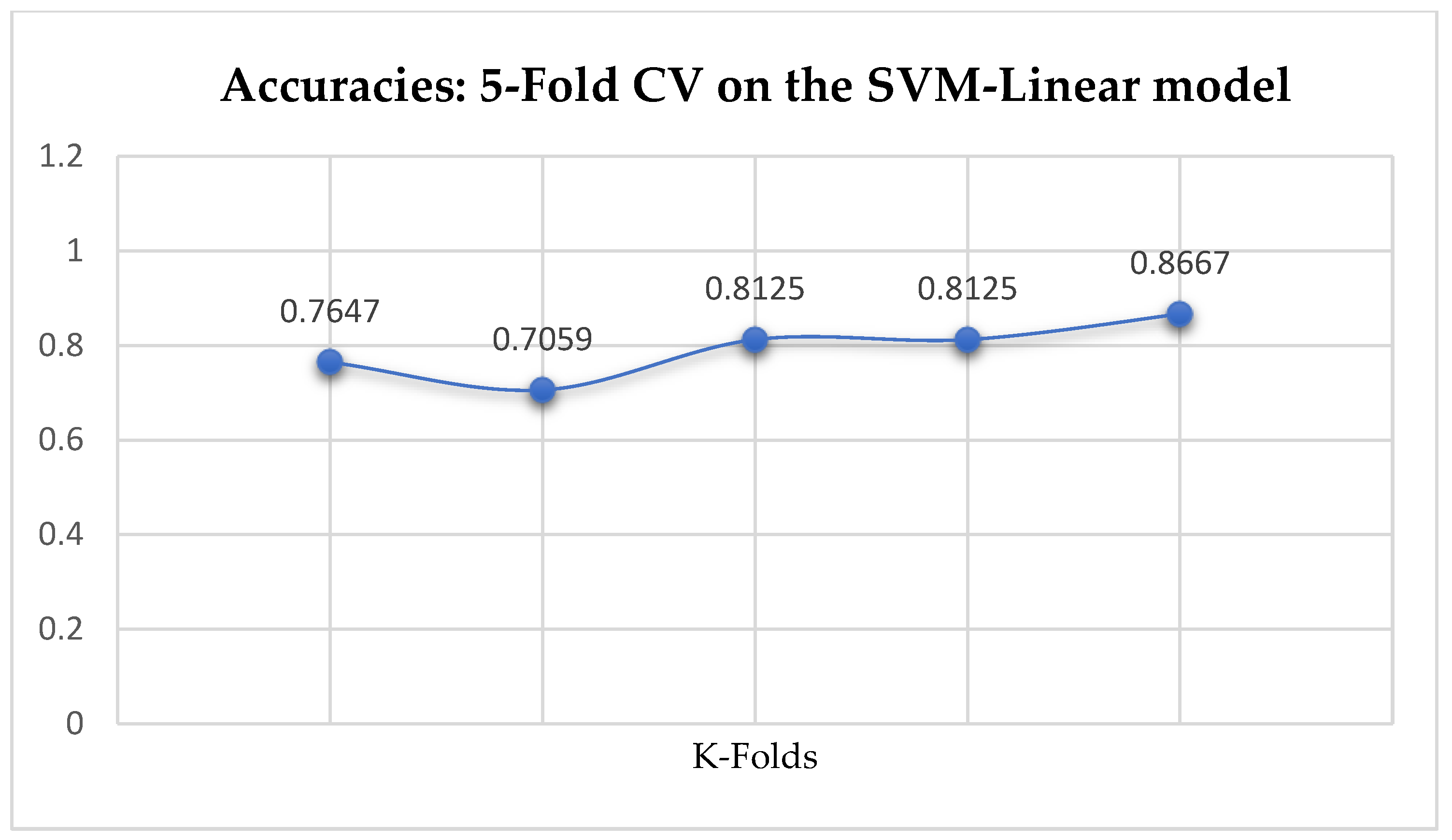
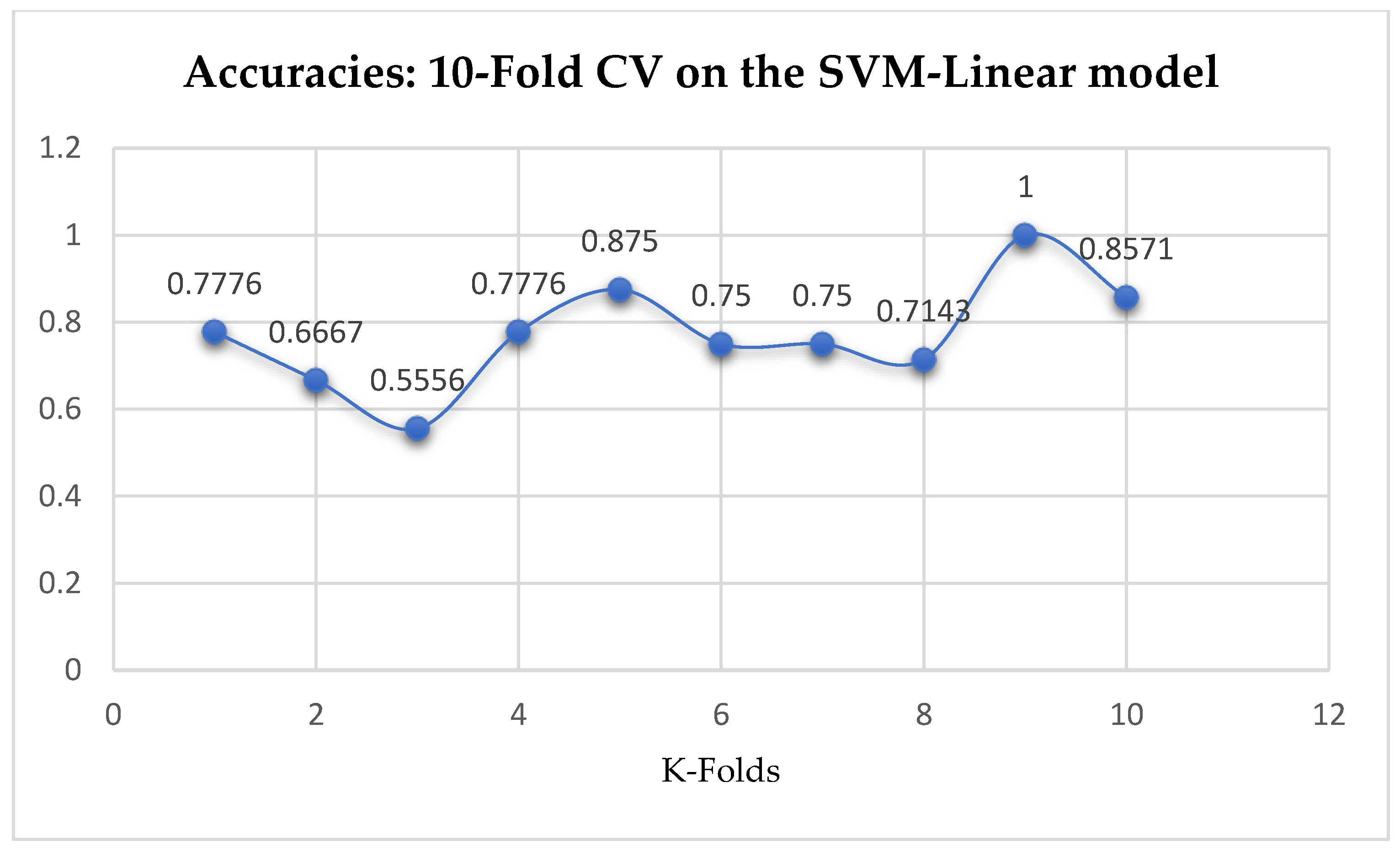
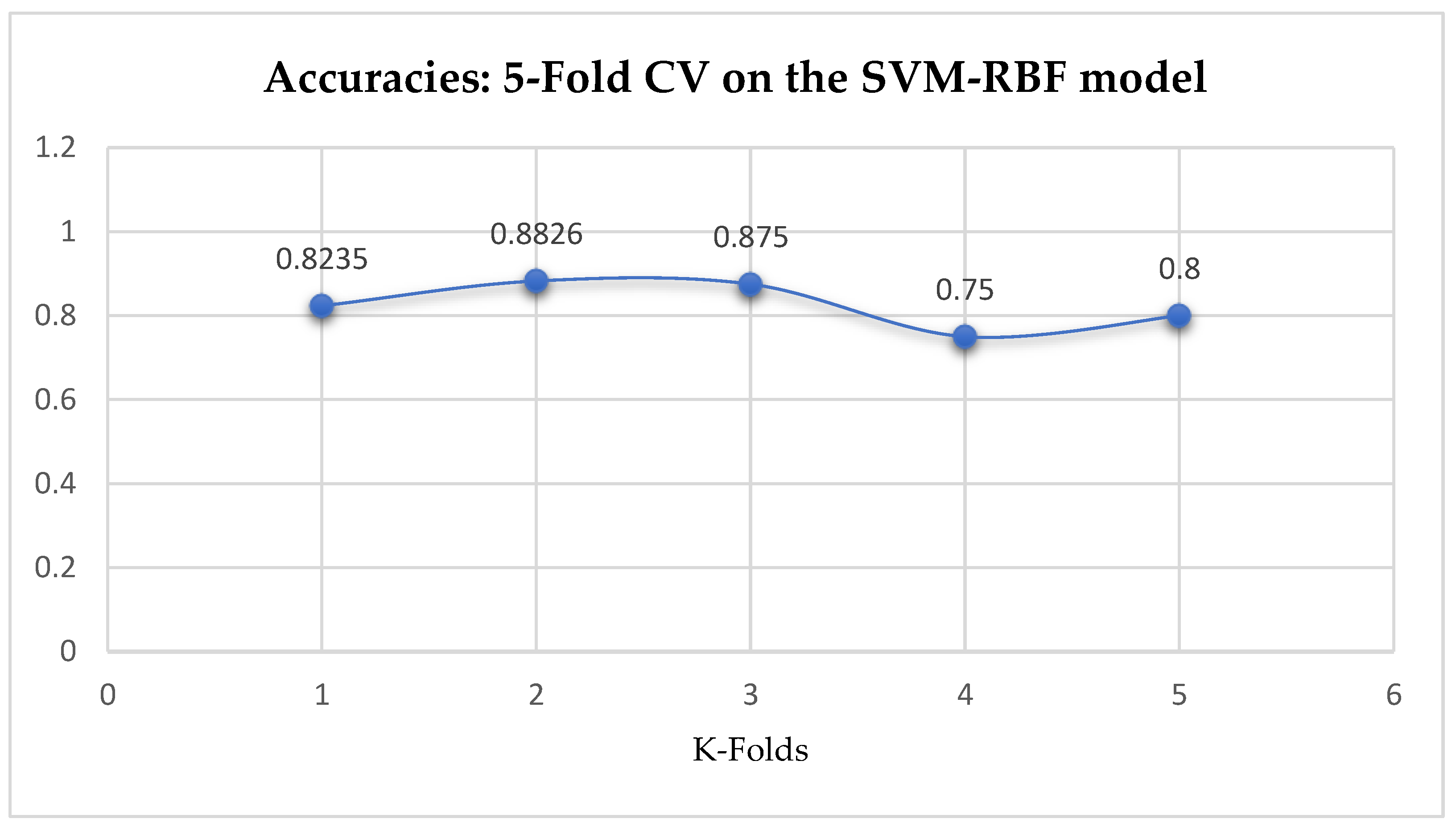
Among the SVM classifiers, The SVM-Linear achieved a mean accuracy of 79.25% based on the 5-Fold Cross-Validation as shown in Table 17. We can observe a decrease in accuracy from 79.25% to 77.24% after the 10-Fold CV as seen from Table 17. Also, based on the K-Fold Cross-Validation, without Grid Searching, the baseline model, LR outperformed the SVM-Linear model as seen from Table 17. 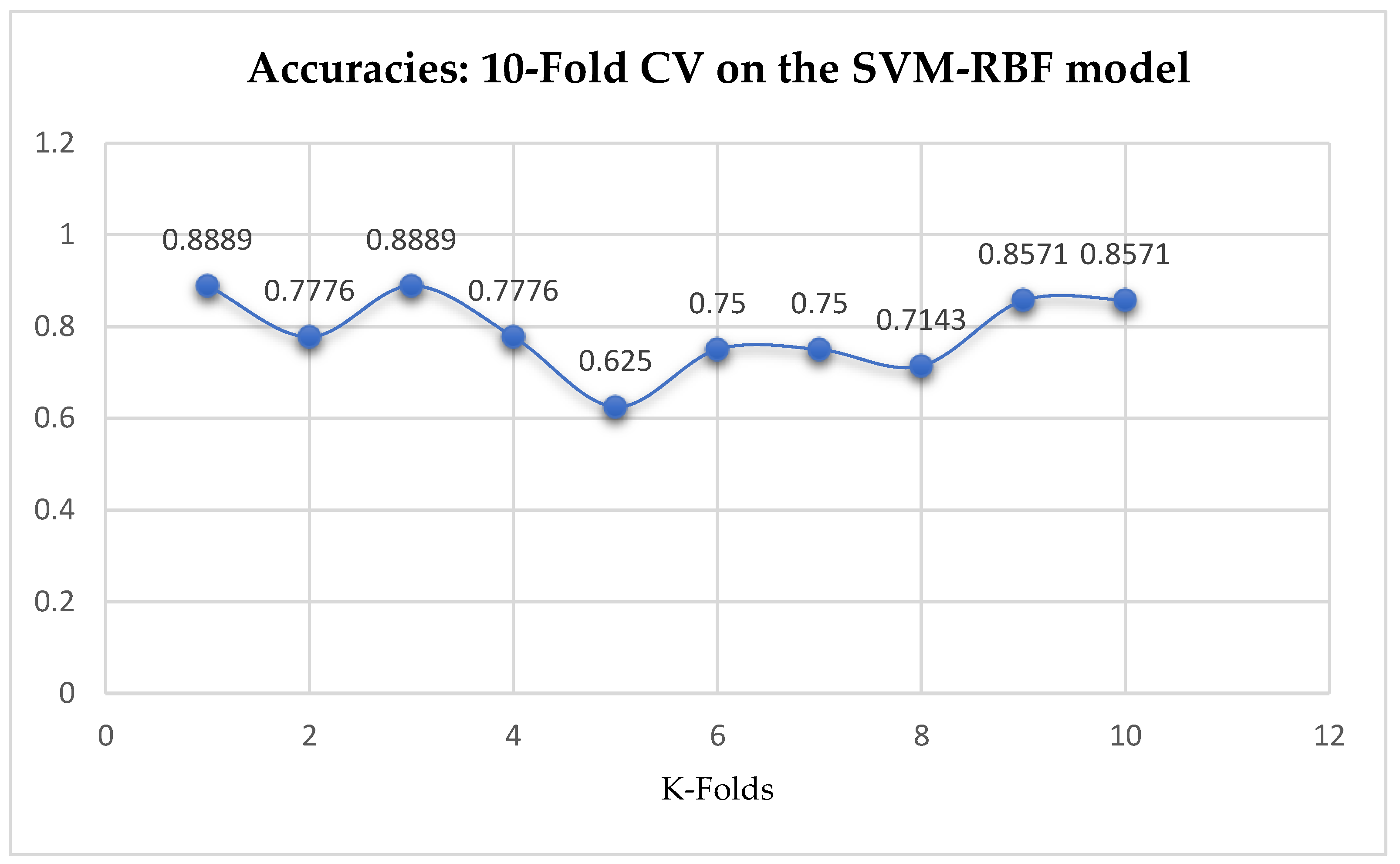The SVM-RBF classifier achieved a mean accuracy of 82.62% based on the 5-Fold Cross-Validation as seen from Table 17. With the 10-Fold Cross-Validation, the SVM-RBF classifier achieved a mean accuracy of 78.87% as seen from Table 17. We can observe a decrease in accuracy from 82.62% to 78.87% after the 10-Fold CV by the SVM-RBF classifier as shown in Table 17. By comparing the SVM-RBF with the LR model, based on the 5-Fold Cross-Validation, the SVM-RBF model outperformed the LR model. 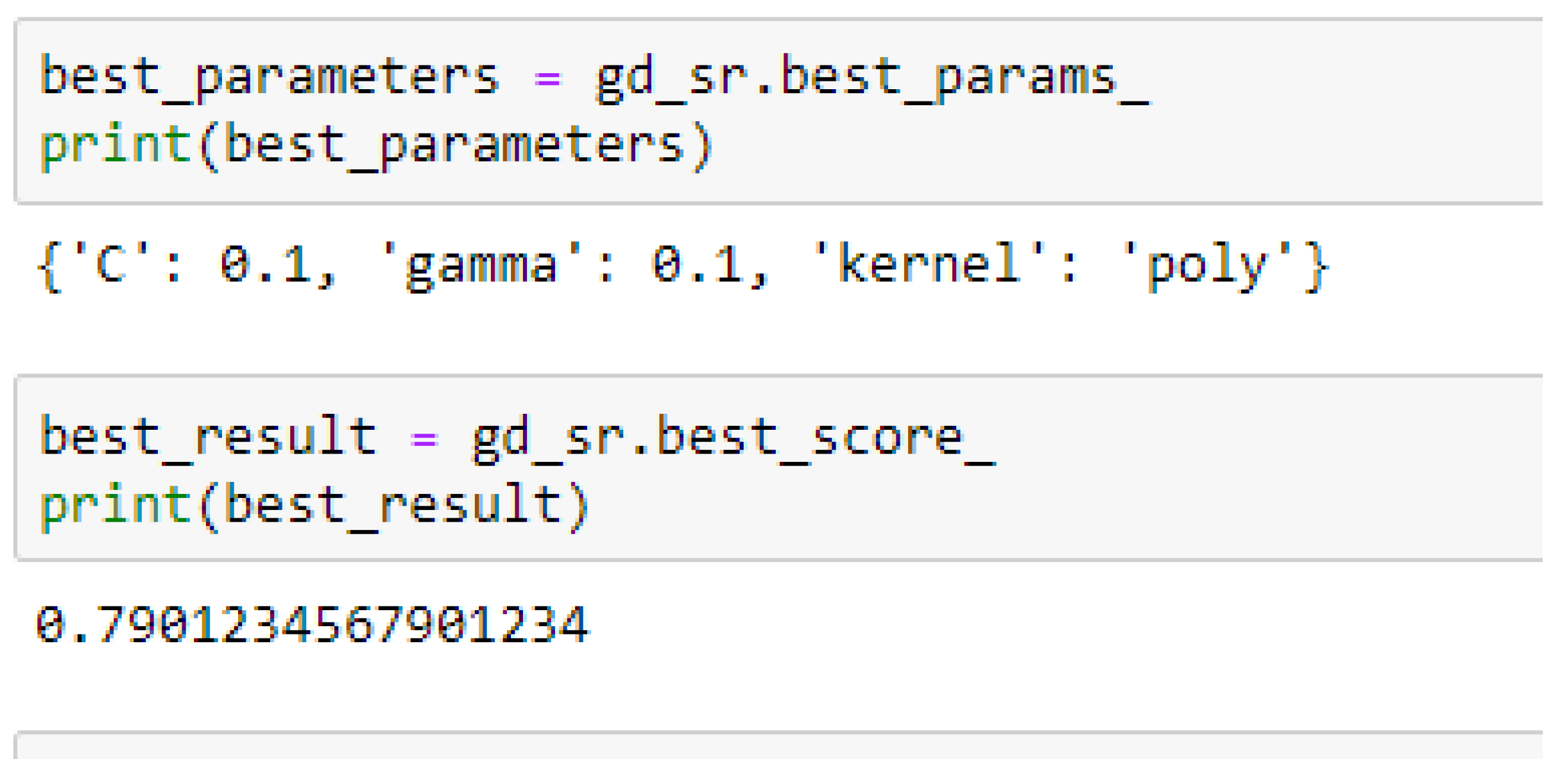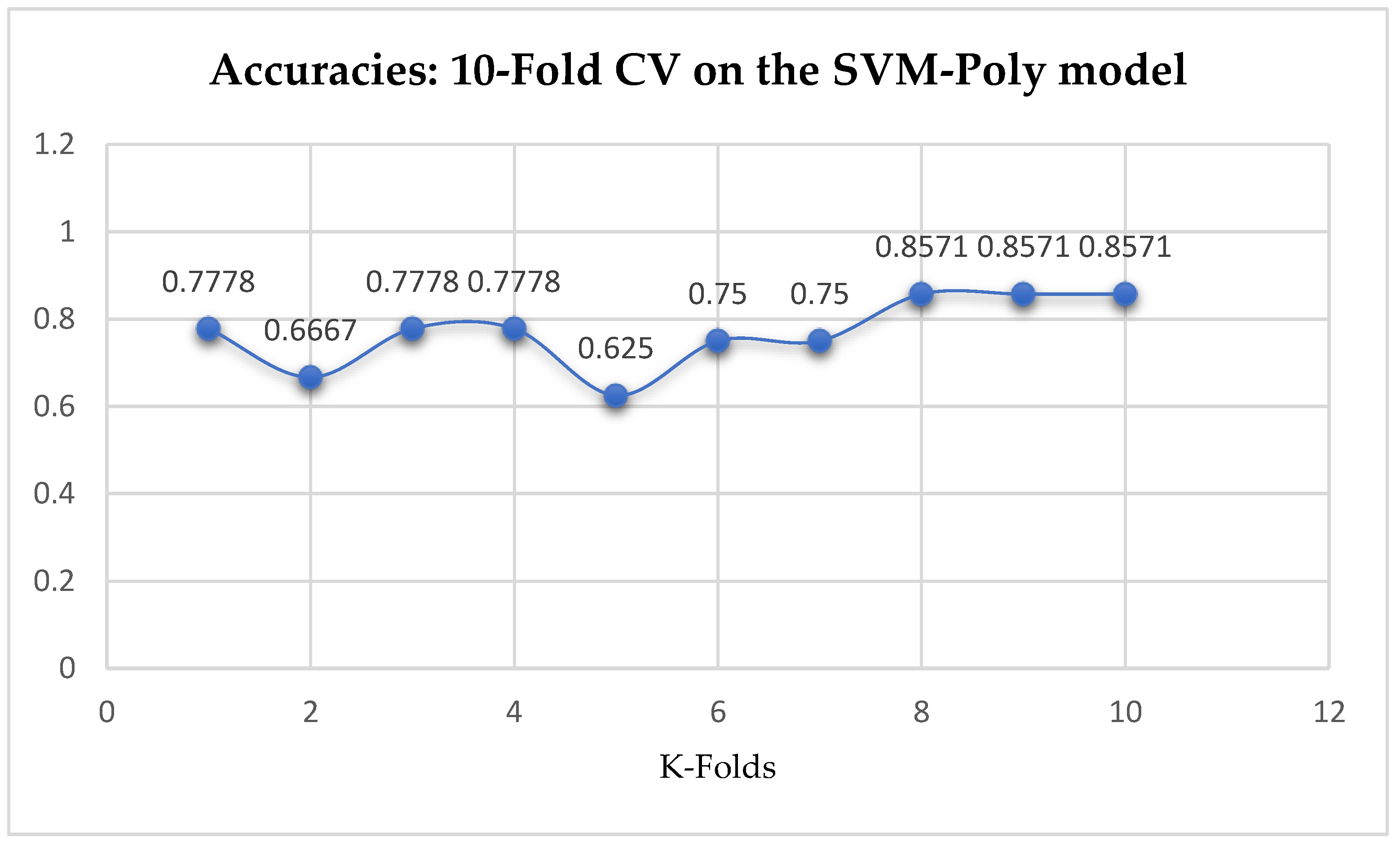Whereas, based on the 10-Fold Cross-Validation, the LR model slightly outperformed the SVM-RBF model as seen from Table 17. Finally, the SVM-Poly classifier achieved a mean accuracy of 76.42% based on the 5-Fold Cross-Validation as seen from Table 17. With the 10-Fold Cross-Validation, the SVM-Poly classifier achieved a mean accuracy of 76.96%. We can observe an increase in accuracy from 76.42% to 76.96% after the 10-Fold CV by the SVM-Poly classifier as seen from Table 17. By comparing the SVM-Poly model with the LR model, based on the K-Fold Cross-Validation, without grid search, the LR model outperformed the SVM-Poly model.

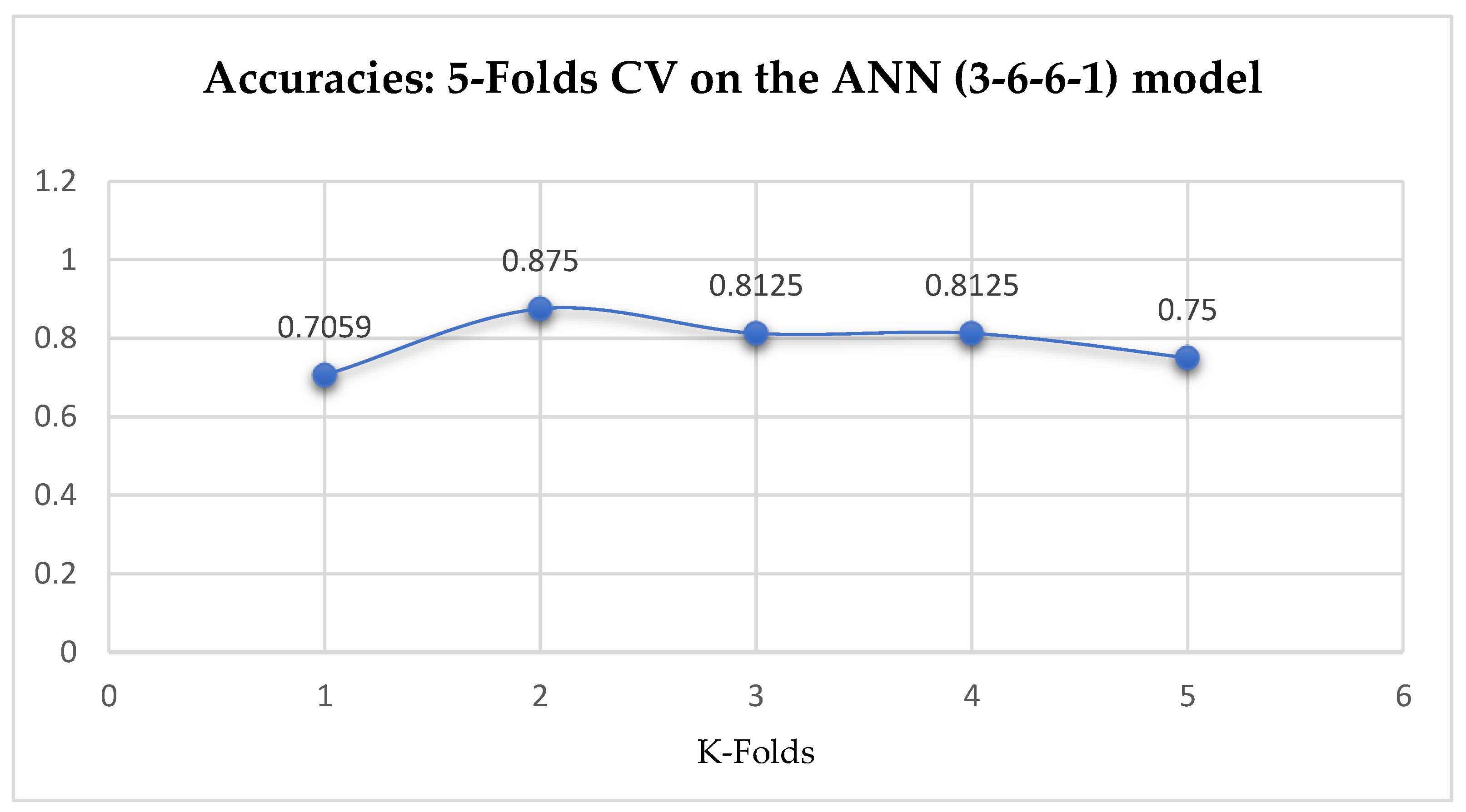
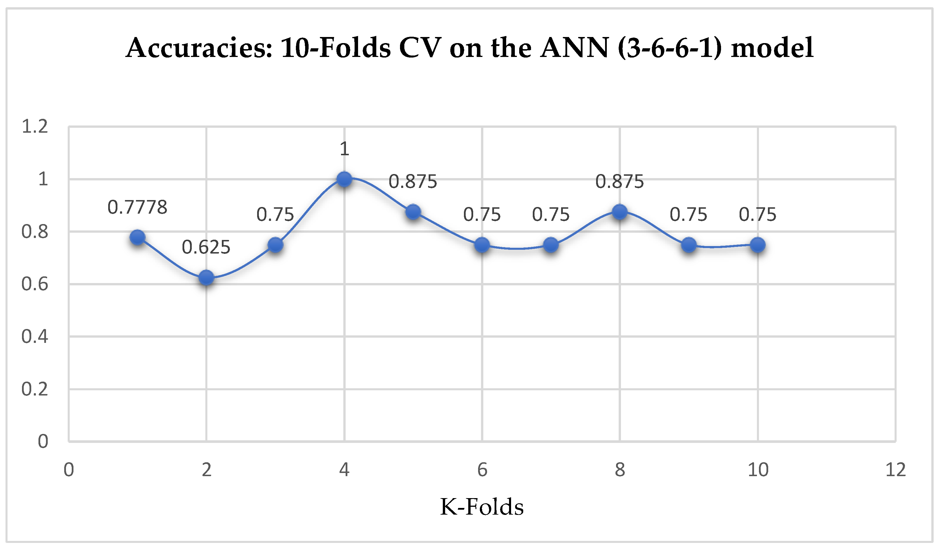
Lastly, based on the K-Fold Cross-Validation, without Grid Searching, the ANN (3-6-6-1) model achieved a mean accuracy of 79.12% based on the 5-Fold Cross-Validation as seen from Table 17. With the 10-Fold Cross-Validation, the ANN (3-6-6-1) model achieved a mean accuracy of 79.03% as seen from Table 17. 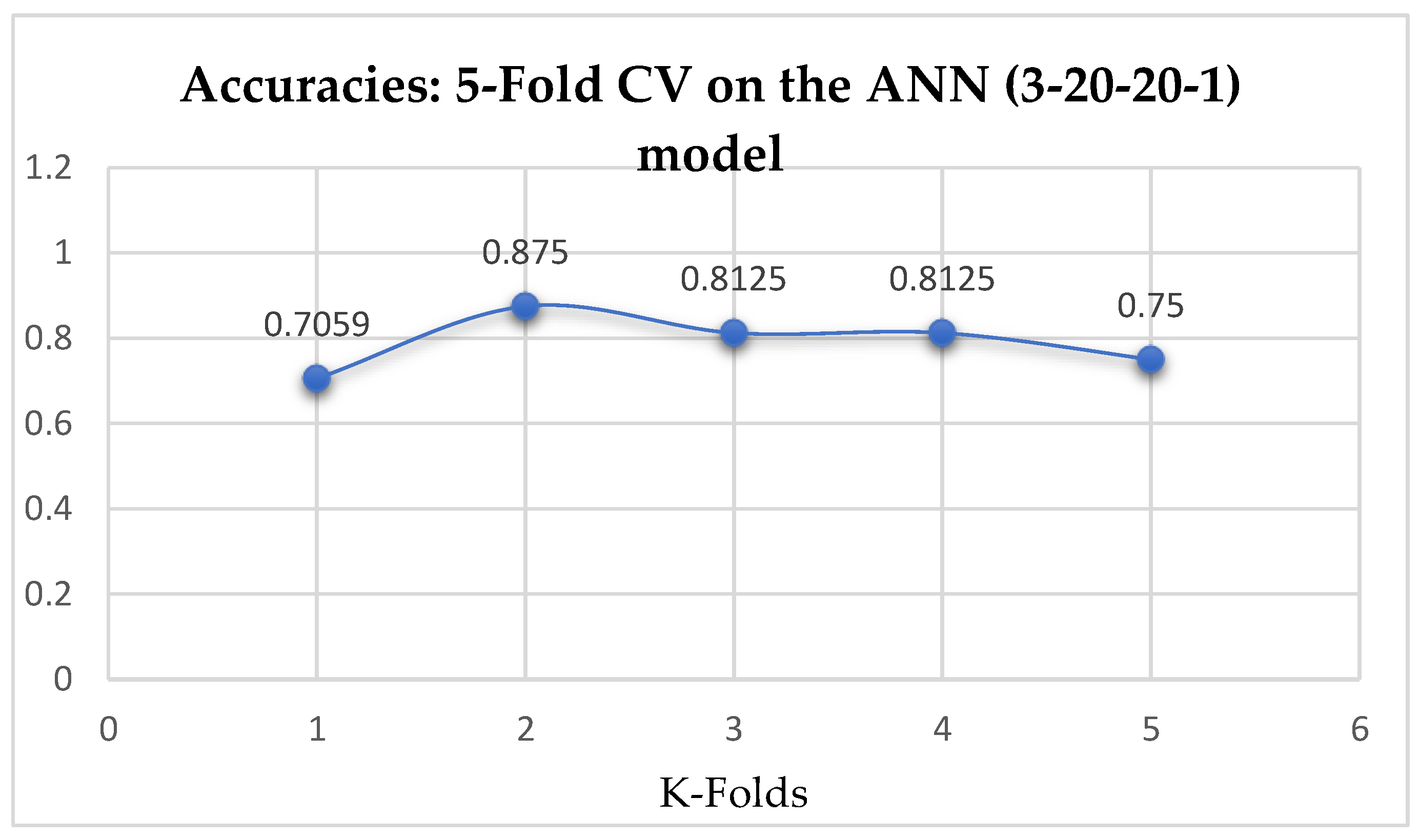We can observe a decrease in accuracy from 79.12% to 79.03% after the 10-Fold CV by the ANN (3-6-6-1) model as shown in Table 17. Also, the ANN (3-20-20-1) model achieved a mean accuracy of 79.12% based on the 5-Fold Cross-Validation as seen from Table 17. With the 10-Fold Cross-Validation, the ANN (3-20-20-1) model achieved a mean accuracy of 79.03%. We can observe a decrease in accuracy from 79.12% to 79.03% after the 10-Fold CV by the ANN (3-6-6-1) model as shown in Table 17. By comparing the ANN models with the LR model, based on the K-Fold Cross-Validation, without grid search, the LR model outperformed both the ANN models as seen from Table 17.

With the analysis in this current work, based on performing 5- and 10-Fold Cross-Validation without grid searching (as summarized in Table 17), we then state that the assumption concluded in the work of Christodoulou et al. [33] that they found no evidence of superior performance of machine learning over Logistic Regression when performing clinical prediction modeling is somehow quite true.

We observed that, among the ML algorithms, the SVM-RBF outperformed all the other ML models, which achieved an accuracy of 82.62% based on the 5-Fold Cross-Validation with grid searching as shown in Table 17. Whereas, based on the 10-Fold Cross-Validation without grid searching, the ANN models outperformed the other ML models, by which both the ANN models achieved an accuracy of 79.03% as shown in Table 17.

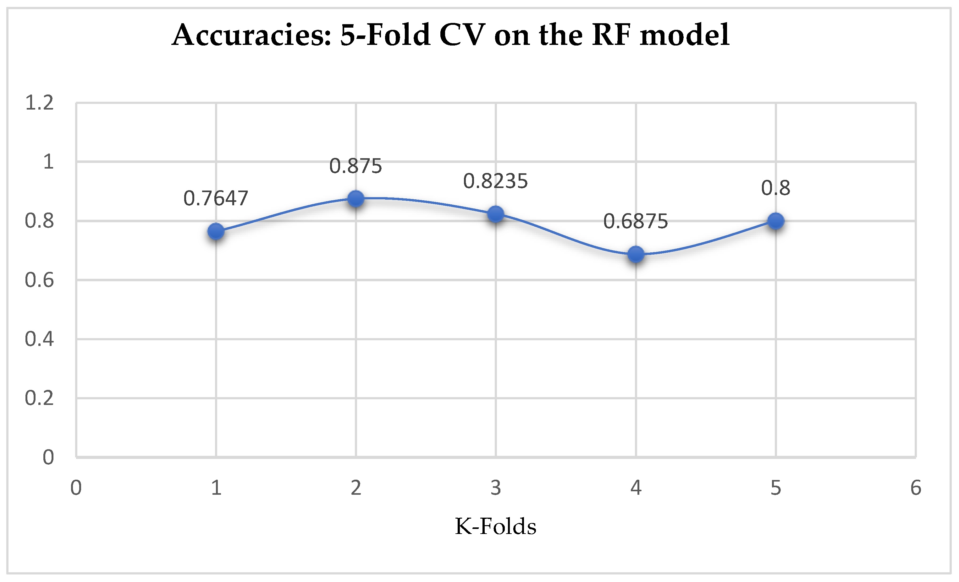
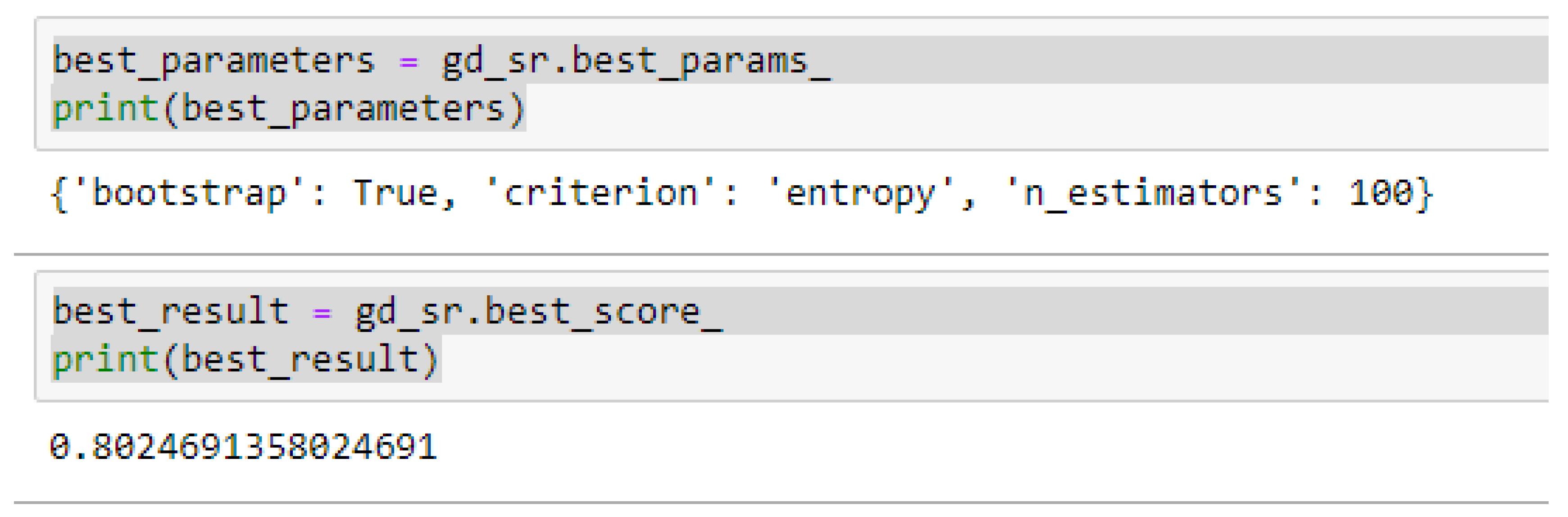
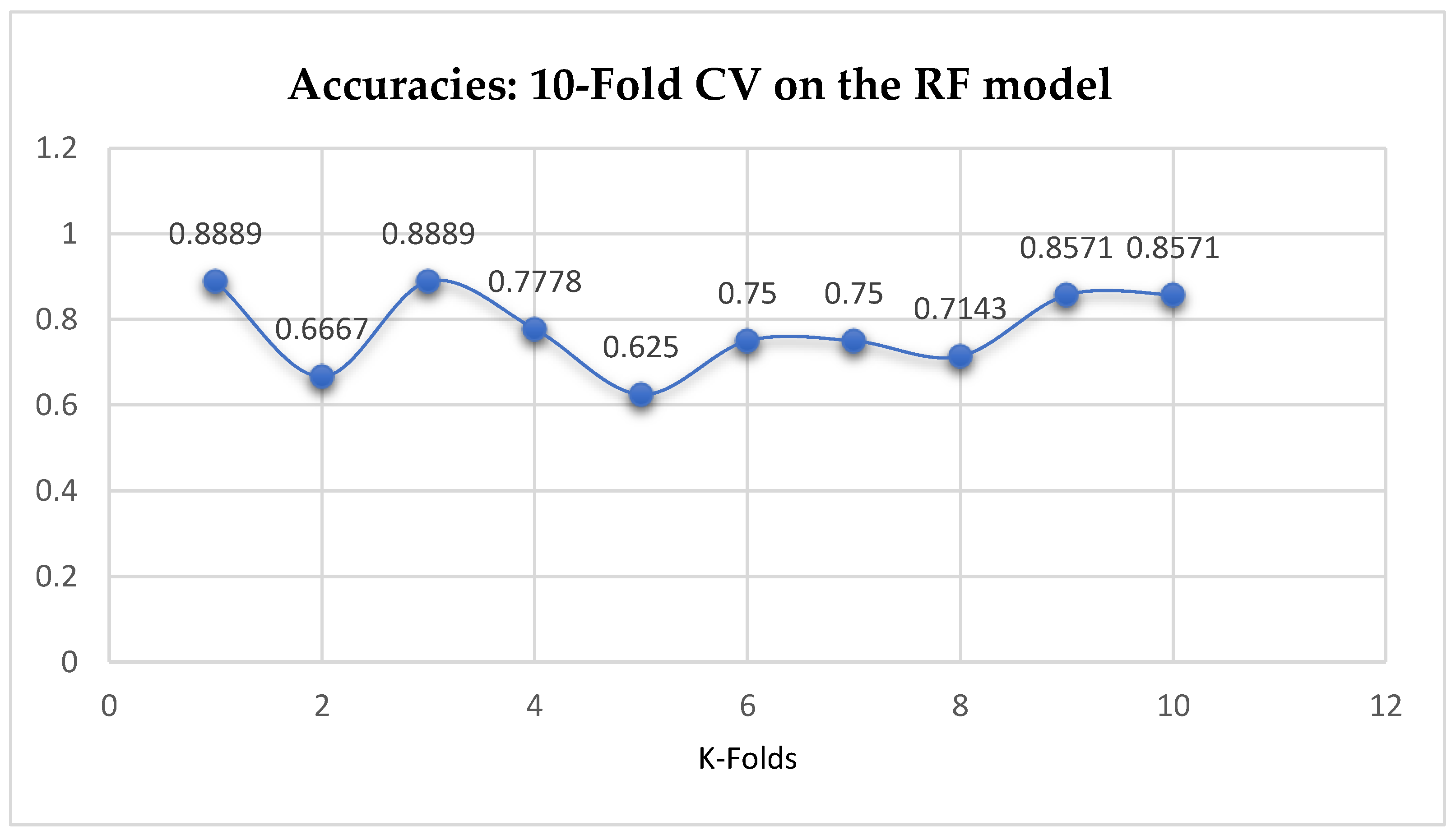
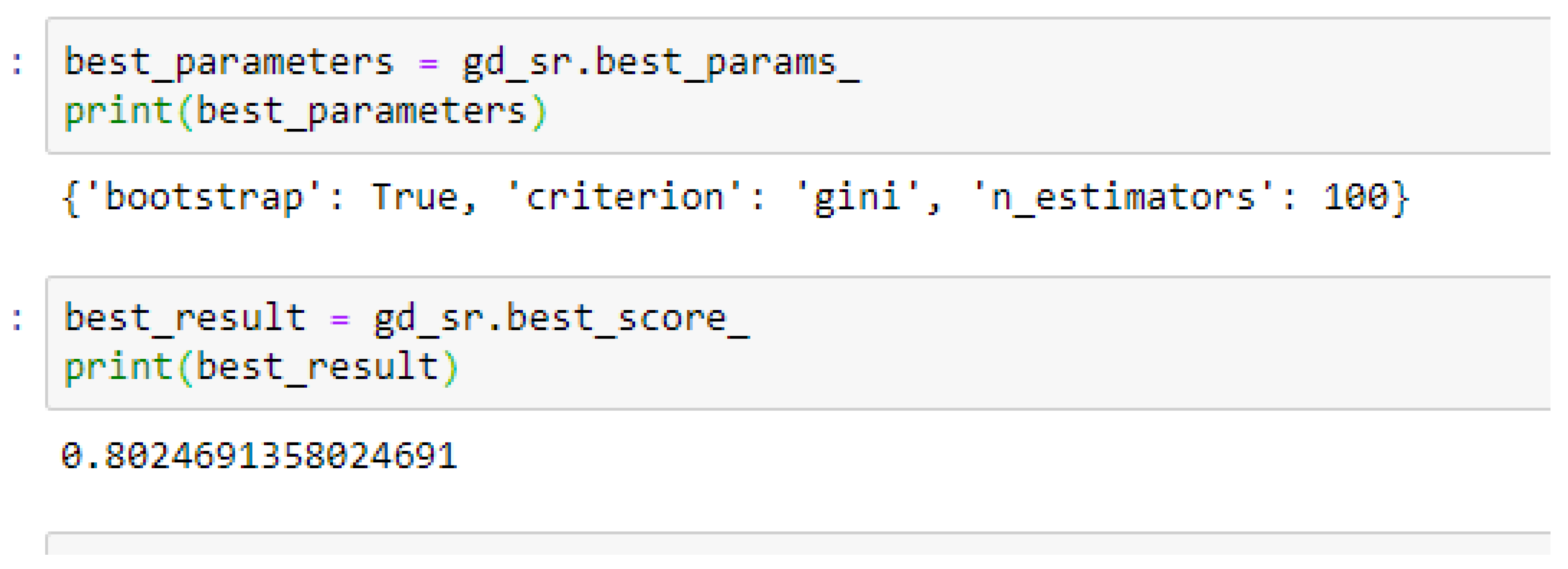
The second category of our experiment was to improve on the performances of the ML models, and then find the best parameters with the highest accuracies. We achieved these by performing grid search with 5- and 10-Fold Cross-Validation. After running the grid search algorithms, the performance of the RF model improved from 79.01%, and 77.76% to 80.25% based on both the 5- and 10-Fold Cross-Validation as seen from Table 15 and Table 16 respectively. We observed that, based on 10-Fold CV with grid search, the RF model outperformed the LR model as seen from Table 15 and Table 16 respectively.

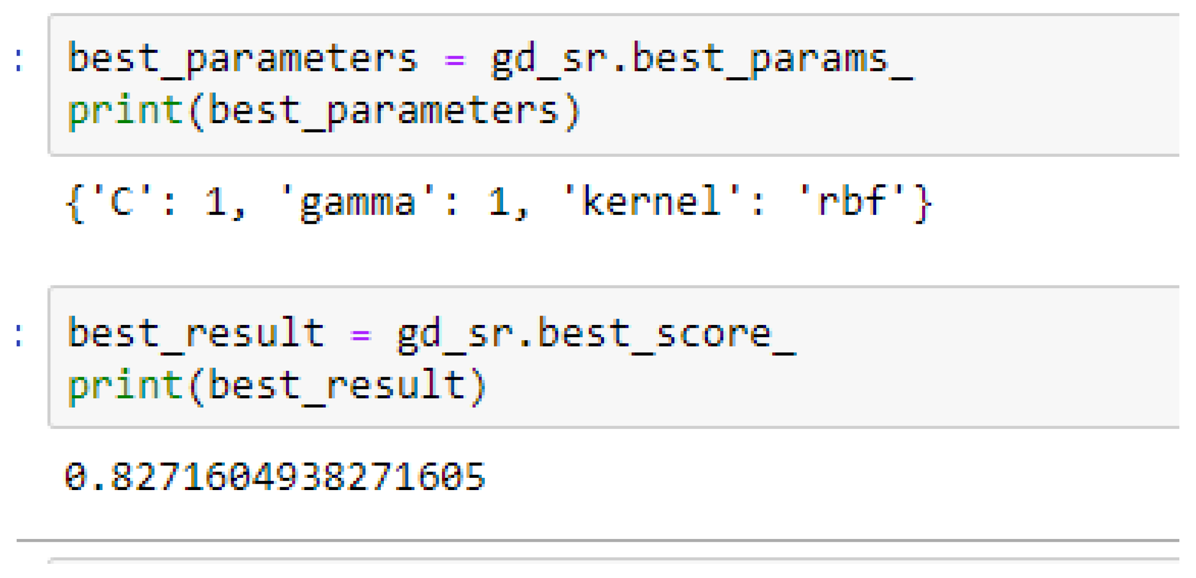
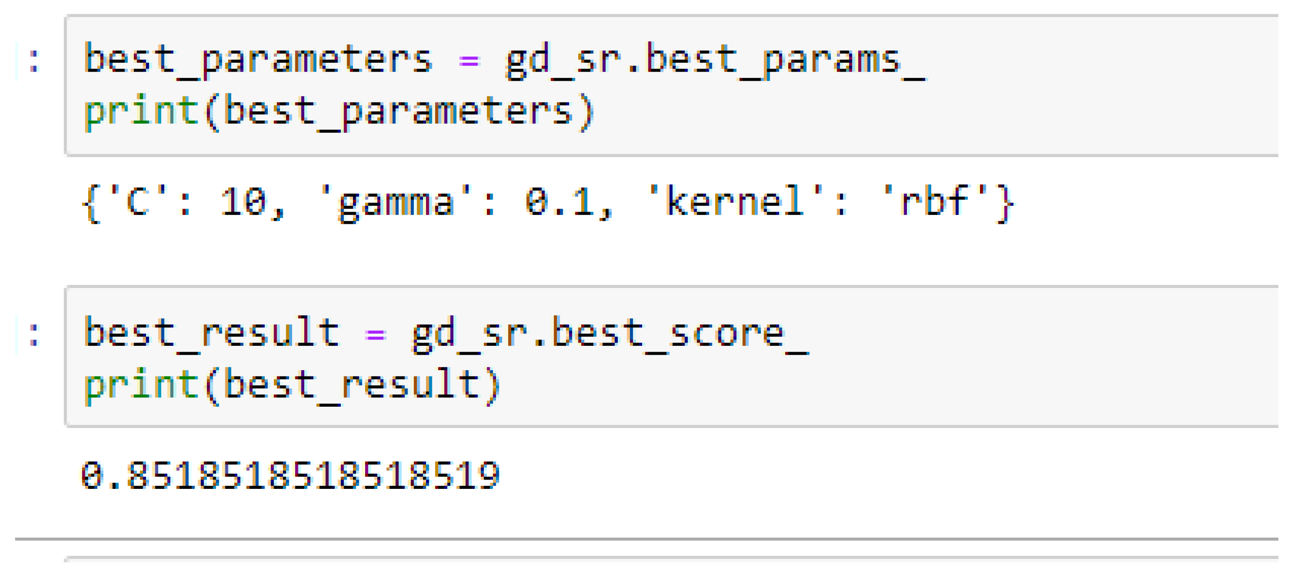
Among the SVM classifiers, we also observed that, the accuracies of the SVM-Linear did not improve significantly after performing the grid search with the K-Fold CV (as shown in Table 15 and Table 16) to that of the K-Fold CV without grid search as shown in Table 17. Again, the LR model outperformed the SVM-Linear model. We observed an improvement of the SVM-RBF model from 82.62%, and 78.87% to 82.72, and 85.19% based on the 5- and 10-Fold Cross-Validation as seen from Table 15 and Table 16 respectively. By comparing the SVM-RBF model with the LR model, after performing grid search with K-Fold CV, the SVM-RBF model then outperformed the LR model as seen from (Table 15 and Table 16) and Table 17 respectively.

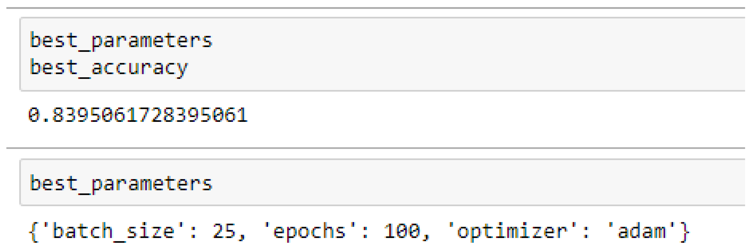
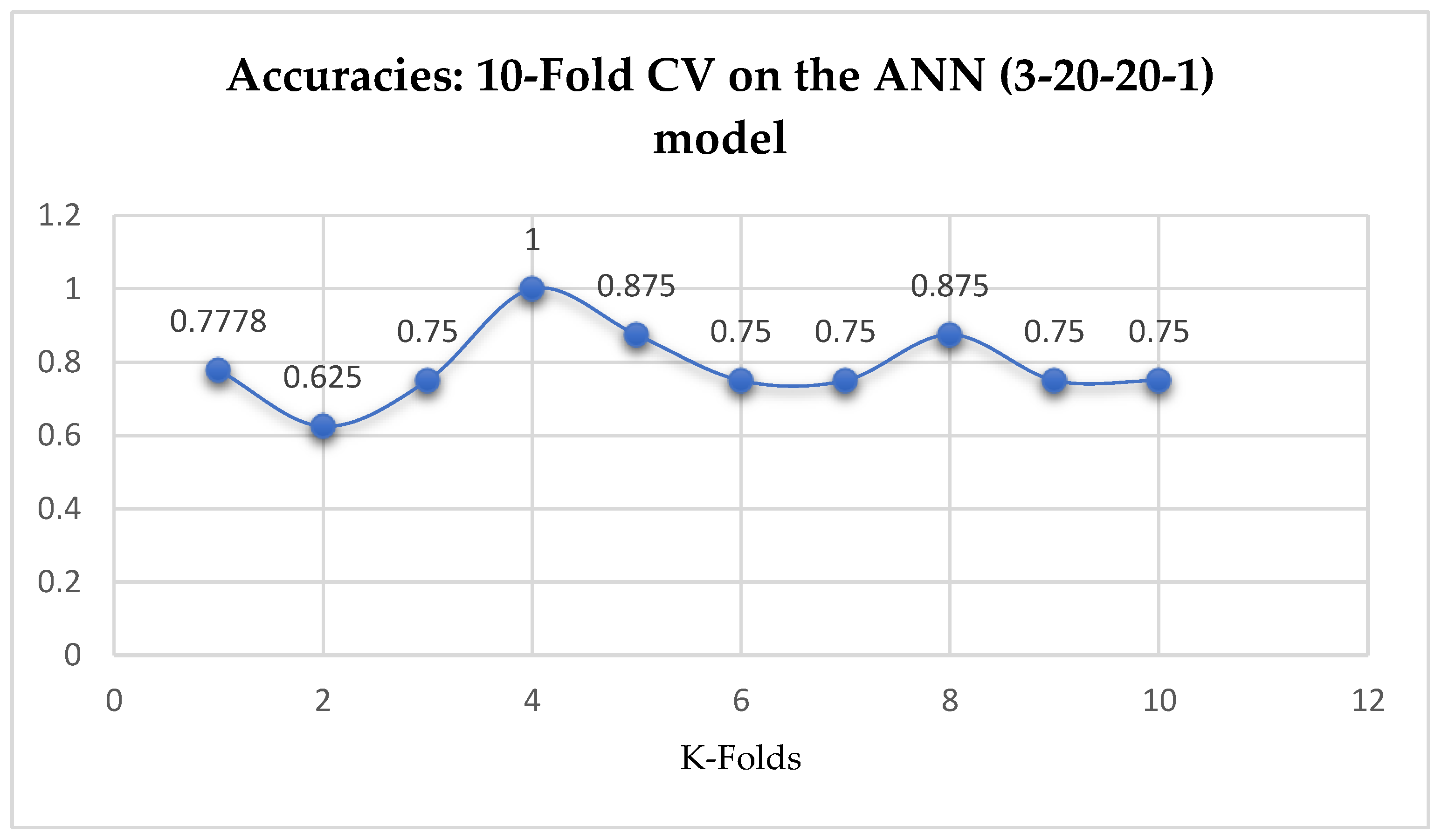
Finally, among the ANN models, the accuracies of the ANN (3-6-6-1) improved from 79.12%, and 79.03% to 85.19%, and 86.42% based on the 5- and 10-Fold Cross-Validation as seen from Table 15 and Table 16 respectively. Also, the accuracies of the ANN (3-20-20-1) improved from 79.12%, and 79.03% to 83.95%, and 85.19% based on the 5- and 10- Fold Cross-Validation as seen from Table 15 and Table 16 respectively.

By comparing the ML models as seen from Table 15 and Table 16, we observed that, by performing 5- or 10-Fold Cross-Validation based on the RF model, the best parameters did not change much, setting bootstrap to true, criterion to either entropy or gini, and the number of trees to 100, really improved the RF model in both cases as seen from Figure 16 and Figure 17 respectively.

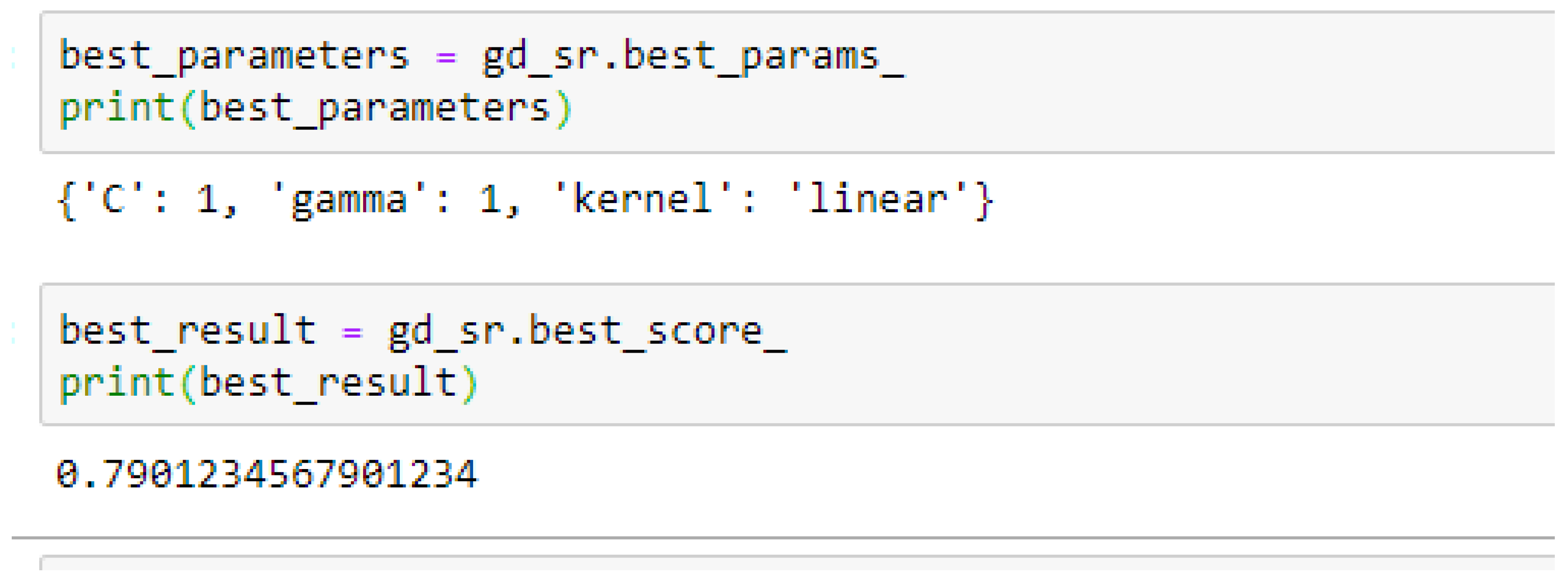
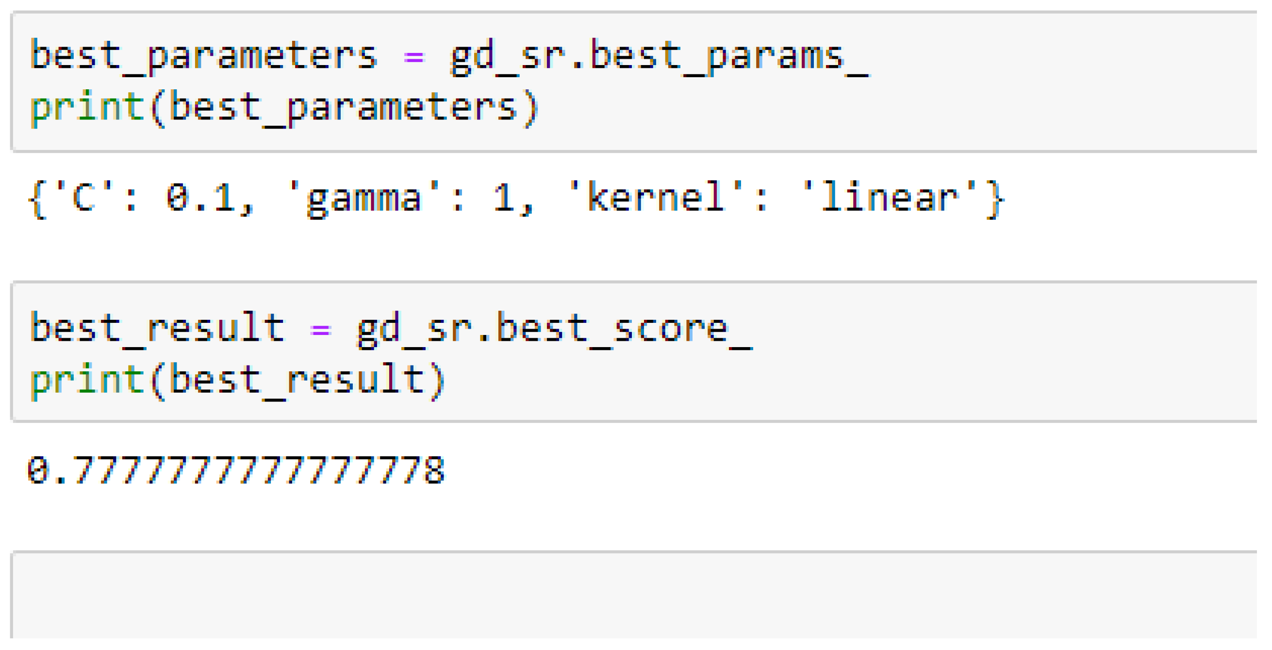
Among the SVM classifiers, the SVM-Linear model performed better when both the cost function and gamma had the same value of 1, based on the 5-Fold Cross-Validation, as compared with the 10-Fold Cross-Validation when the value of the cost function was 0.1 and gamma was 1, as shown in Table 15 and Table 16 respectively. 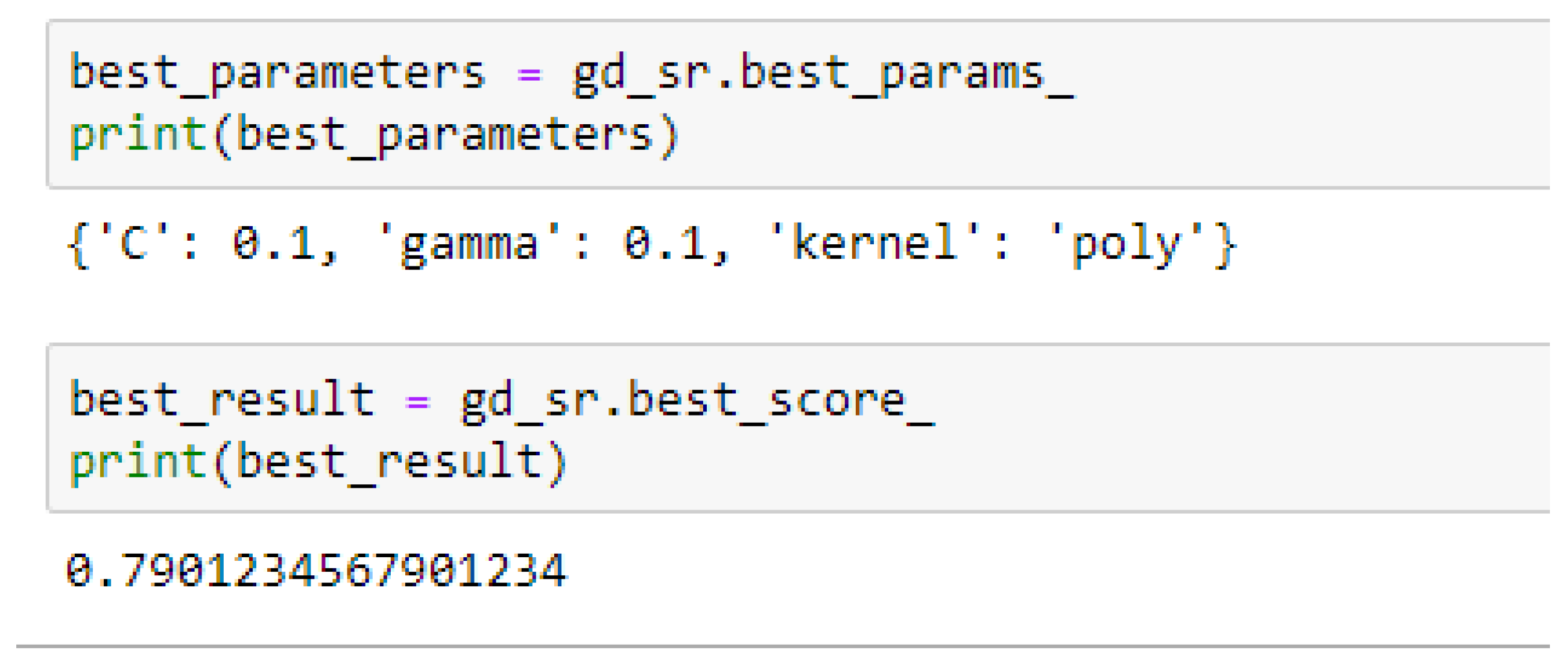The SVM-RBF model performed better based on the 10-Fold Cross-Validation when the values of the cost function and the gamma were 10 and 0.1 respectively, as compared with the 5-Fold Cross-Validation when both the cost function and the gamma had the same value of 1, as seen from Table 15. For the SVM-Poly model, the model gave the same accuracy in both cases, based on the 5- and 10- Fold Cross-validation when the values of the cost function and the gamma were 0.1 and 0.1 respectively.

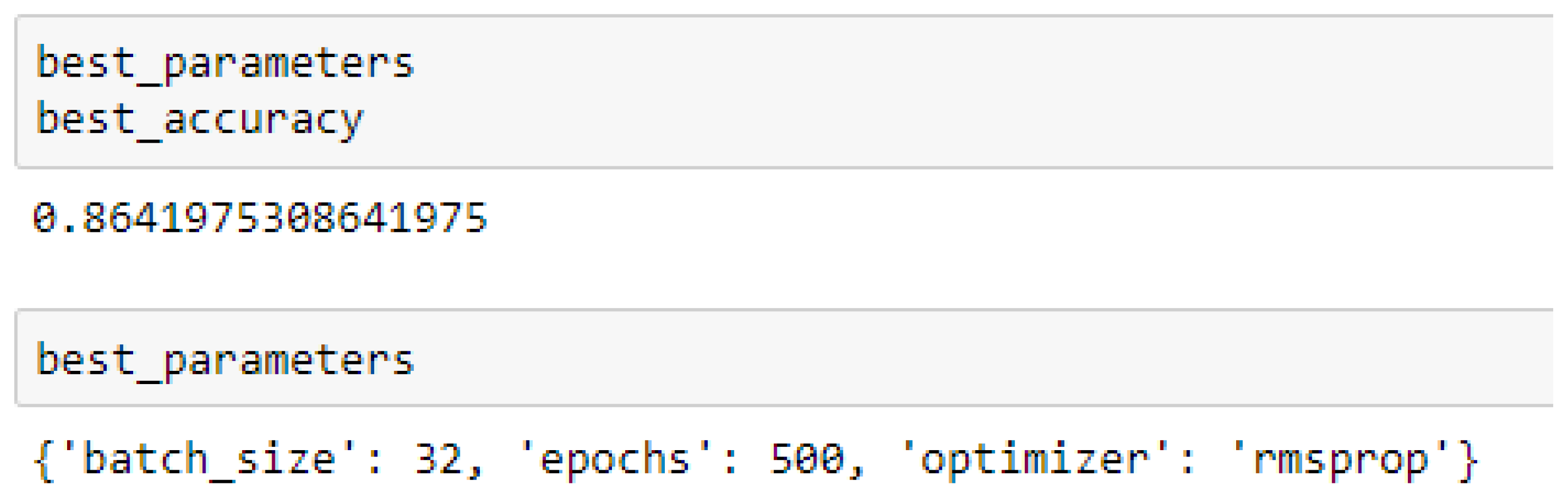
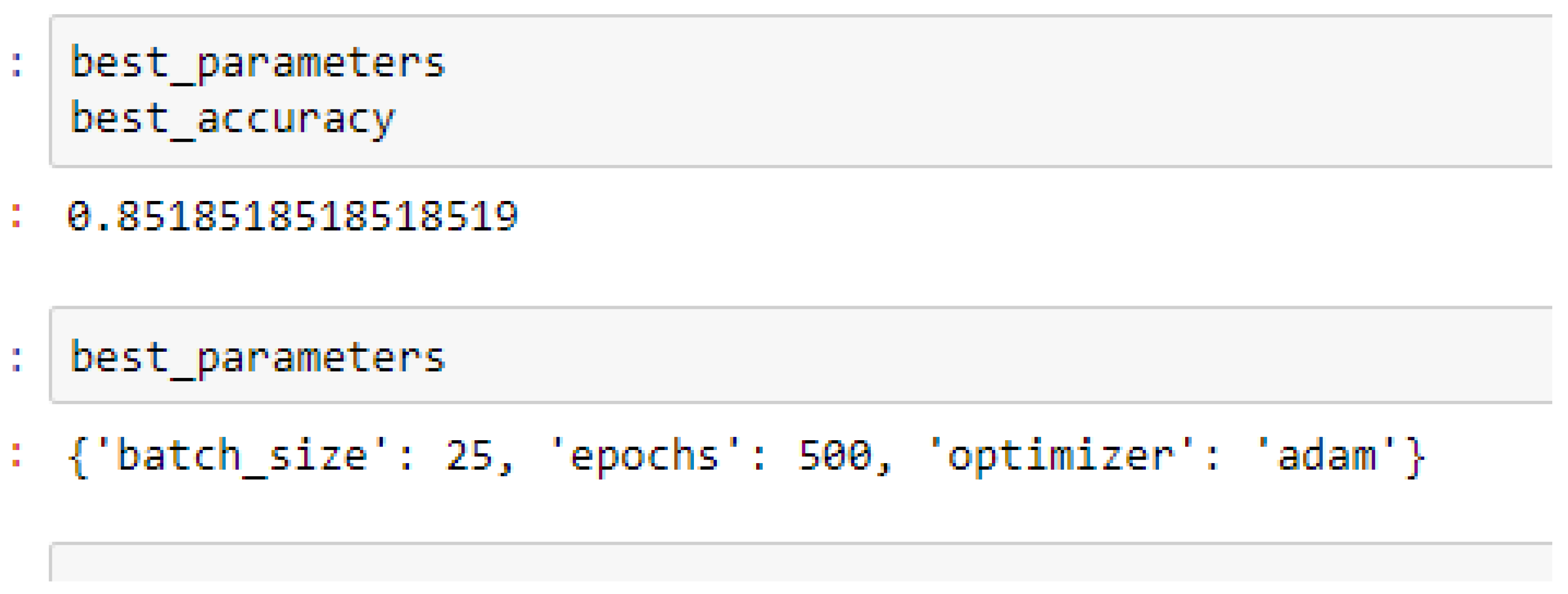
The ANN (3-6-6-1) model performed better based on the 10-Fold Cross-Validation when the values of the batch size, epochs were 32 and 500 respectively, and the optimizer was the rmsprop (root mean square) as compared with the 5-Fold Cross-Validation when the values of the batch size, epochs were 25 and 500 respectively, and the optimizer was Adam, as seen from Table 15 and Table 16 respectively. And also, the ANN (3-20-20-1) model performed better based on the 10-Fold Cross-Validation when the values of the batch size, epochs were 25 and 500 respectively, and the optimizer was Adam, as compared with the 5-Fold Cross-Validation when the values of the batch size, epochs were 25 and 100 respectively, and the optimizer was the Adam, as seen from Table 15 and Table 16 respectively.

Based on the 5- and 10- Fold Cross-Validation after grid searching the RF, SVM-RBF and ANN models achieved more than 80% as seen from Table 15 and Table 16 respectively. The RF, SVM-RBF and ANN models outperformed the baseline model based on the 10-Fold Cross-Validation with grid search. Overall, in terms of accuracies, the ANN (3-6-6-1) model outperformed all the other models, achieving 85.19% and 86.42% based on the 5- and 10-Fold Cross-Validation respectively, after running grid search algorithms.

Based on the findings of the ML algorithms, we have achieved the objective of this work to predict kyphosis disease. We compared the results of our ML models with the LR model, we found out that, LR is also capable in making clinical predictions, and for that matter, must not be overlooked, as can be verified from Table 17. Based on the small sample size used in this work, we took advantage of K-Fold Cross-Validation to evaluate the models, and also took advantage of grid search to obtained the best parameters for the models.

For the ML Algorithms in making clinical predictions (kyphosis), the following are the implications based on our findings:

• In using RF model to making clinical predictions, it is better to set bootstrap to true, both gini or entropy can be tried as the criterion, and the value of 100 can be tried as the starting point for the number of trees.
• In SVM-Linear model, given the value of gamma equals 1, the values of (0.1 or 1) can be tried as the cost function when making clinical predictions.
• In SVM-RBF model, the highest value for the cost function can be 10, while the lowest value can be 1, and the highest value for the gamma can be 1 while the lowest value can be 0.1, when making clinical predictions to obtain high accuracies.
• In using the SVM-Poly to making clinical predictions, the value of 0.1 can be tried for both the cost function and the gamma.
• In making clinical predictions based on ANN model, the values of the batch size and the epochs can be tried with 32 and 500 respectively, and the optimizer can either be rmsprop or Adam. However, most preferably, the rmsprop optimizer can firstly be experimented with.

The highest accuracies achieved by the ANN models, as seen from Table 15 and Table 16, imply that the number of the neurons may have increased the size of the data, since ML algorithms demand big sample size to be trained. Finally, the findings of our results show that, by performing 10-Fold Cross-Validation with grid search, will actually bring out the best model with the highest accuracy, as seen from Figure 17.

Our current work serves as an opportunity for other researchers to improve upon the accuracies, and also research on how to obtain big data on kyphosis disease in order to explore the predictive power of the proposed ML algorithms. The findings of our work would also trigger further research into the comparison between the Logistic regression and ML algorithms in clinical prediction problems.

In future works, the ML models can be extended to make other clinical predictions with big data, so as to further observe and compare the performances of the ML models as confined in this current work.

5. Conclusions

In this current research work, we have applied three different machine learning algorithms, which are, Random Forest, Support Vector Machines, and Artificial Neural Network to predict kyphosis disease. We observed overall accuracies of the models between 79%–85%, and 77%–86% as seen from Table 15 and Table 16, based on the 5- and 10-Fold Cross-Validation after running grid search respectively. The RF, SVM-RBF and ANN models achieved accuracies of more than 80% based on 5- and 10- Fold Cross-Validation (CV). Overall, the ANN (3-6-6-1) model outperformed all the other models, achieving 85.19% and 86.42% based on the 5- and 10-Fold Cross-Validation respectively. We observed that RF, SVM-RBF and ANN models are capable to detect and predict kyphosis disease after a patient had undergone surgery or operation. We suggest that machine learning should be adopted and used as an essential and critical tool across the maximum spectrum of answering biomedical questions. We, therefore, proposed that RF, SVM-RBF, and ANN, as machine learning algorithms, should be used to detect and predict kyphosis disease after a patient had undergone surgery or operation. In future works, more machine learning algorithms can be tested in order to improve on the accuracy in predicting kyphosis disease.

References

1. Vinitha, S.; Sweetlin, S.; Vinusha, H.; Sajini, S. Disease Prediction Using Machine Learning Over Big Data. Comput. Sci. Eng. Int. J. 2018, 8. [Google Scholar] [CrossRef]
2. Tahmooresi, M.; Afshar, A.; Bashari, R.; Babak, B.N.; Bamiah, K.M. Early Detection of Breast Cancer Using Machine Learning Techniques. J. Telecommun. Electron. Comput. Eng. 2018, 10, 21–27. [Google Scholar]
3. Ayon, D. Machine Learning Algorithms: A Review. Int. J. Comput. Sci. Inf. Technol. 2016, 7, 1174–1179. [Google Scholar]
4. Richert, W.; Coelho, L.P. Building Machine Learning Systems with Python; Packt Publishing Ltd.: Birmingham, UK, 2013; ISBN 978-1-78216-140-0. [Google Scholar]
5. Ali, E.; Feng, W. Breast Cancer classification using Support Vector Machine and Neural Network. Int. J. Sci. Res. 2013, 5, 2319–7064. [Google Scholar]
6. Chen, S.T.; Hsiao, Y.H.; Huang, Y.L.; Kuo, S.J.; Tseng, H.S.; Wu, H.K.; Chen, D.R. Comparative analysis of logistic regression, support vector machine and artificial neural network for the differential diagnosis of benign and malignant solid breast tumors by the use of three-dimensional power Doppler imaging. Korean J. Radiol. 2009, 10, 464–471. [Google Scholar] [CrossRef] [PubMed]
7. Simons, A. Using Artificial Intelligence to Improve Early Breast Cancer Detection. Available online: https://www.csail.mit.edu/news/using-artificial-intelligence-improve-early-breast-cancer-detection (accessed on 26 June 2019).
8. Abdullah, A.; Yaakob, A.; Ibrahim, Z. Prediction of Spinal Abnormalities Using Machine Learning Techniques. In Proceedings of the 2018 International Conference on Computational Approach in Smart Systems Design and Applications, Kuching, Serawak, Malaysia, 15–17 August 2018; pp. 1–6. [Google Scholar] [CrossRef]
9. Alaa, B.E.; Sefer, K. Diabetes Diagnosis Using Machine Learning. IJCSMC 2019, 8, 36–41. [Google Scholar]
10. Shao, Y.E.; Hou, C.D.; Chiu, C.C. Hybrid intelligent modelling, schemes for heart disease classification. Appl. Soft Comput. 2014, 14, 47–52. [Google Scholar] [CrossRef]
11. Jaymin, P.; Tejal, U.; Samir, P. Heart Disease Prediction Using Machine learning and Data Mining Technique. IJCSC 2016, 7, 129–137. [Google Scholar] [CrossRef]
12. Animesh, H.; Subrata, K.M.; Amit, G.; Arkomita, M.; Asmita, M. Heart Disease Diagnosis and Prediction Using Machine Learning and Data Mining Techniques: A Review. Adv. Comput. Sci. Technol. 2017, 10, 2137–2159. [Google Scholar]
13. Kavitha, K.S.; Ramakrishnan, K.V.; Manoj, K.S. Modelling and Design of Evolutionary Neural Network for Heart Disease Detection. Int. J. Comput. Sci. Issues 2010, 7, 272–283. [Google Scholar]
14. Noura, A. Heart Diseases Diagnoses Using Artificial Neural Network. Netw. Complex Syst. 2015, 5, 7–11. [Google Scholar]
15. Mrudula, G.; Kapil, W.; Snehlata, D. Decision Support System for Heart Disease Based on Support Vector Machine and Artificial Neural Network. In Proceedings of the 2010 International Conference on Computer and Communication Technology, Bradford, UK, 29 June–1 July 2010; pp. 17–19. [Google Scholar] [CrossRef]
16. Ayeldeen, H.; Elfattah, M.A.; Shaker, O.; Hassanien, A.E.; Kim, T.H. Case-Based Retrieval Approach of Clinical Breast Cancer Patients. In Proceedings of the 2015 3rd International Conference on Computer, Information and Application, Qingdao, China, 28–29 November 2015; pp. 38–41. [Google Scholar]
17. Prachi, D.S.; Ram, N.G. Comparative Analysis of Artificial Neural Network and Support Vector Machine Classification for Breast Cancer Detection. Int. Res. J. Eng. Technol. 2015, 2, 2114–2119. [Google Scholar]
18. Kuo, C.Y.; Yu, L.C.; Chen, H.C.; Chan, C.L. Comparison of Models for the Prediction of Medical Costs of Spinal Fusion in Taiwan Diagnosis-Related Groups by Machine Learning Algorithms. Healthc. Inform. Res. 2018, 24, 29–37. [Google Scholar] [CrossRef] [PubMed]
19. John, M.C.; Trevor, J.H. Statistical Models in S; Wadsworth and Brooks/Cole: Pacific Grove, CA, USA, 1992. [Google Scholar]
20. Sperandei, S. Understanding logistic regression analysis. Biochem. Med. 2014, 24, 12–18. [Google Scholar] [CrossRef] [PubMed]
21. Understanding Logistic Regression. Available online: https://towardsdatascience.com/understanding-logistic-regression-9b02c2aec102 (accessed on 6 August 2019).
22. Breiman, L. Random Forests. Mach. Learn. 2001, 45, 5–32. [Google Scholar] [CrossRef] [Green Version]
23. Neural Designer. Available online: https://www.neuraldesigner.com/blog/what_is_advanced_analytics (accessed on 7 June 2019).
24. Vapnik, V.N. Statistical Learning Theory; Wiley: New York, NY, USA, 1998. [Google Scholar]
25. Van, G.T.; Suykens, J.A.; Baesens, B. Benchmarking Least Squares Support Vector Machine Classifiers. Mach. Learn. 2004, 54, 5. [Google Scholar] [CrossRef]
26. Hasan, M.; Nasser, M.; Pal, B.; Ahmad, S. Support Vector Machine and Random Forest Modeling for Intrusion Detection System (IDS). J. Intell. Learn. Syst. Appl. 2014, 6, 45–52. [Google Scholar] [CrossRef] [Green Version]
27. Prajapati, G.L.; Patle, A. On Performing Classification Using SVM with Radial Basis and Polynomial Kernel Functions. In Proceedings of the 3rd International Conference on Emerging Trends in Engineering and Technology, Goa, India, 19–21 November 2010; pp. 512–515. [Google Scholar] [CrossRef]
28. Mathematics of Neural Networks. Available online: https://juxt.pro/blog/posts/neural-maths.html (accessed on 26 July 2019).
29. Kingma, D.; Ba, J. Adam: A method for stochastic optimization. arXiv 2014, arXiv:1412.6980. [Google Scholar]
30. k-Fold Cross-Validating Neural Networks. Available online: https://chrisalbon.com/deep_learning/keras/k-fold_cross-validating_neural_networks/ (accessed on 26 July 2019).
31. Cross-Validation: Evaluating Estimator Performance. Available online: https://scikit-learn.org/stable/modules/cross_validation.html (accessed on 26 July 2019).
32. Min, C.; Yixue, H.; Kai, H.; Lu, W.; Lin, W. Disease Prediction by Machine Learning Over Big Data from Healthcare Communities. Special Section on Healthcare Big Data. IEEE Acess 2017. [Google Scholar] [CrossRef]
33. Christodoulou, E.; Jie, M.; Gary, S.C.; Ewout, W.S.; Jan, Y.V.; Ben, V.C. A systematic review shows no performance benefit of machine learning over logistic regression for clinical prediction models. J. Clin. Epidemiol. 2019, 110, 12–22. [Google Scholar] [CrossRef] [PubMed]
Figure 1. (a) Representation of Artificial Intelligence and its subfields; (b) Components of machine learning.
Applsci 09 03322 g001
Figure 2. (a) A normal spine (without kyphosis); (b) Patient with abnormal spine (kyphosis).
Applsci 09 03322 g002
Figure 3. A screenshot of the kyphosis data (first top 10 records) after the kyphosis class column has been transformed in to 0′s and 1′s.
Applsci 09 03322 g003
Figure 4. Structure of a Random Forest [21].
Applsci 09 03322 g004
Figure 5. (a) Structure of a Neural Network; (b) A Three-layered Artificial Neural Network.
Applsci 09 03322 g005
Figure 6. The flowchart of the Artificial Neural Network (ANN) model implementation.
Applsci 09 03322 g006
Figure 7. (a) The Architectural Structure of the ANN model (3-6-6-1); (b) The Architectural Structure of the ANN model (3-20-20-1).
Applsci 09 03322 g007
Figure 8. (a) The Architectural Structure of the ANN model (3-6-6-1) with 73 trainable parameters; (b) The Architectural Structure of the ANN model (3-20-20-1) with 521 trainable parameters.
Applsci 09 03322 g008
Figure 9. A flowchart of typical cross-validation workflow in model training [31].
Applsci 09 03322 g009
Figure 10. The illustration of a K-Fold cross-validation process [31].
Applsci 09 03322 g010
Figure 11. The distribution of the kyphosis disease representing absent or present.
Applsci 09 03322 g011
Figure 12. (a) The correlations between the features in the data; (b) The patterns of the kyphosis identified among the three input features (Age, Start, Number).
Applsci 09 03322 g012
Figure 13. The boxplot of kyphosis against Age feature to detect outliers.
Applsci 09 03322 g013
Figure 14. (a) The boxplot of kyphosis against Number feature to detect outliers; (b) The boxplot of kyphosis against Start feature to detect outliers.
Applsci 09 03322 g014
Figure 15. The accuracies achieved by the Folds after performing 5-Fold Cross-Validation on the LR model.
Applsci 09 03322 g015
Figure 16. The accuracies achieved by the Folds after performing 10-Fold Cross-Validation on the LR model.
Applsci 09 03322 g016
Figure 17. The accuracies achieved by the Folds after performing 5-Fold Cross-Validation on the RF model.
Applsci 09 03322 g017
Figure 18. The best parameters with obtained after performing Grid Search with 5-Fold Cross-Validation on the RF model.
Applsci 09 03322 g018
Figure 19. The accuracies achieved by the Folds after performing 10-Fold Cross-Validation on the RF model.
Applsci 09 03322 g019
Figure 20. The best parameters with obtained after performing Grid Search with 10-Fold Cross-Validation based on the RF model.
Applsci 09 03322 g020
Figure 21. The accuracies achieved by the Folds after performing 5-Fold Cross-Validation on the Support Vector Machines (SVM)-Linear model.
Applsci 09 03322 g021
Figure 22. The best parameters with obtained after performing Grid Search with 5-Fold Cross-Validation on the SVM-Linear model.
Applsci 09 03322 g022
Figure 23. The accuracies achieved by the Folds after performing 10-Fold Cross-Validation on the SVM-Linear model.
Applsci 09 03322 g023
Figure 24. The best parameters with obtained after performing Grid Search with 10-Fold Cross-Validation on the SVM-Linear model.
Applsci 09 03322 g024
Figure 25. The accuracies achieved by the Folds after performing 5-Fold Cross-Validation on the SVM-Radial Basis Function (RBF) model.
Applsci 09 03322 g025
Figure 26. The best parameters with obtained after performing a grid search with 5-Fold Cross-Validation on the SVM-RBF model.
Applsci 09 03322 g026
Figure 27. The accuracies achieved by the Folds after performing 10-Fold Cross-Validation on the SVM-RBF model.
Applsci 09 03322 g027
Figure 28. The best parameters with obtained after performing grid search with 10-Fold Cross-Validation on the SVM-RBF model.
Applsci 09 03322 g028
Figure 29. The accuracies achieved by the Folds after performing 5-Fold Cross-Validation on the SVM-Poly model.
Applsci 09 03322 g029
Figure 30. The best parameters with obtained after performing grid search with 5-Fold Cross-Validation on the SVM-poly model.
Applsci 09 03322 g030
Figure 31. The accuracies achieved by the Folds after performing 10-Fold Cross-Validation on the SVM-Poly model.
Applsci 09 03322 g031
Figure 32. The best parameters with obtained after performing grid search with 10-Fold Cross-Validation on the SVM-Poly model.
Applsci 09 03322 g032
Figure 33. The accuracies achieved by the Folds after performing 5-Fold Cross-Validation on the ANN (3-6-6-1) model.
Applsci 09 03322 g033
Figure 34. The best parameters with obtained after performing grid search with 5-Fold Cross-Validation on the ANN (3-6-6-1) model.
Applsci 09 03322 g034
Figure 35. The accuracies achieved by the Folds after performing 10-Fold Cross-Validation on the ANN (3-6-6-1) model.
Applsci 09 03322 g035
Figure 36. The best parameters with obtained after performing grid search with 10-Fold Cross-Validation on the ANN (3-6-6-1) model.
Applsci 09 03322 g036
Figure 37. The accuracies achieved by the Folds after performing 5-Fold Cross-Validation on the ANN (3-20-20-1) model.
Applsci 09 03322 g037
Figure 38. The best parameters with obtained after performing grid search with 5-Fold Cross-Validation on the ANN (3-20-20-1) model.
Applsci 09 03322 g038
Figure 39. The accuracies achieved by the Folds after performing 10-Fold Cross-Validation on the ANN (3-20-20-1) model.
Applsci 09 03322 g039
Figure 40. The best parameters with obtained after performing grid search with 10-Fold Cross-Validation on the ANN (3-20-20-1) model.
Applsci 09 03322 g040