Medinoid: Computer-Aided Diagnosis and Localization of Glaucoma Using Deep Learning ^†

Abstract

Glaucoma is a leading eye disease, causing vision loss by gradually affecting peripheral vision if left untreated. Current diagnosis of glaucoma is performed by ophthalmologists, human experts who typically need to analyze different types of medical images generated by different types of medical equipment: fundus, Retinal Nerve Fiber Layer (RNFL), Optical Coherence Tomography (OCT) disc, OCT macula, perimetry, and/or perimetry deviation. Capturing and analyzing these medical images is labor intensive and time consuming. In this paper, we present a novel approach for glaucoma diagnosis and localization, only relying on fundus images that are analyzed by making use of state-of-the-art deep learning techniques. Specifically, our approach towards glaucoma diagnosis and localization leverages Convolutional Neural Networks (CNNs) and Gradient-weighted Class Activation Mapping (Grad-CAM), respectively. We built and evaluated different predictive models using a large set of fundus images, collected and labeled by ophthalmologists at Samsung Medical Center (SMC). Our experimental results demonstrate that our most effective predictive model is able to achieve a high diagnosis accuracy of 96%, as well as a high sensitivity of 96% and a high specificity of 100% for Dataset-Optic Disc (OD), a set of center-cropped fundus images highlighting the optic disc. Furthermore, we present Medinoid, a publicly-available prototype web application for computer-aided diagnosis and localization of glaucoma, integrating our most effective predictive model in its back-end.

1. Introduction

Glaucoma is a progressive optic neuropathy [1], mostly manifesting itself in the area between the optic disc and the macula. The progress of glaucoma usually remains undetected until the optic nerve gets irreversibly damaged. This damage may result in varying degrees of permanent vision loss [2], as illustrated in Figure 1. The earlier glaucoma is diagnosed and treated, the less patients suffer from irreversible disease progress leading to blindness.

The global prevalence of glaucoma is approximately 3–5% for people aged 40–80 years. Specifically, the number of people aged 40–80 years and affected by glaucoma worldwide was estimated to be 64 million in 2013, and this number is expected to increase to 76 million in 2020 and to 112 million in 2040 [3].

As glaucoma progresses, glaucomatous optic disc changes (e.g., Optic Nerve Head (ONH) rim thinning or notching) and parapapillary retinal nerve fiber defects become representative morphological patterns [4,5,6]. As those patterns can be captured by fundus images, an ophthalmologist is able to diagnose glaucoma by manual screening of these images. However, due to individual diversity in optic disc and retina morphology [7,8,9], a human diagnosis usually does not only require fundus images, but also other types of medical images (Retinal Nerve Fiber Layer (RNFL), Optical Coherence Tomography (OCT) disc/macula, perimetry) in order to achieve high accuracy, sensitivity, and specificity values. Furthermore, the whole process of image capturing and manual screening is typically labor intensive and time consuming. Therefore, various Computer-Aided Diagnosis (CAD) techniques have been developed for identifying glaucoma, with the aim of improving the visual interpretation of fundus images by ophthalmologists. The latter type of images is commonly available in hospitals world-wide, given that their acquisition is relatively inexpensive compared to the acquisition of other types of medical images.

In the area of computer-aided glaucoma diagnosis, we can identify two major research directions: (1) glaucoma detection and (2) Optic Disc (OD) segmentation. When scanning the literature on glaucoma detection, we can observe that the accuracy of classification may vary significantly. In particular, as shown in

Table 1. Overview of computer-aided diagnosis for glaucoma. The dataset described covers both training and validation sets. Effectiveness results have been rounded to one decimal place, if applicable. CDR, Cup-to-Disc Ratio; SMO, Sequential Minimal Optimization; ISNT, Inferior, Superior, Nasal, Temporal.

Reference	Approach	Dataset	Classifier	Effectiveness
				Accuracy	Sensitivity	Specificity	AUROC
[17]	Entropy sampling, ensemble learning, and CNNs	DRISHTI-GS,50 images	Softmax logistic classifier	94.1%	92.3%	95.6%	N/A
[10]	Higher order spectra, trace transform, and discrete wavelet transform	Private, 60 images	SVM	92%	90%	93%	N/A
[11]	Pixel intensity values, texture, spectral features, and histogram parameters	Private, 200 images	Naive Bayes, k-NN, and SVM	80%	N/A	N/A	N/A
[13]	Wavelet feature extraction and classification	Private, 63 images	SVM and k-NN	94.7%	97.0%	93.3%	N/A
[18]	Circular Hough transform, edge detection, and optimum channel selection	ORIGAlight, 650 images	NA	CDR error: 0.10	N/A	N/A	N/A
[23]	Morphological operations, geodesic reconstruction by dilation	Private, 50 images	NA	96%	N/A	N/A	N/A
[24]	Region-based active contour model, Hough transform, vessel bend detection, and r-bends information	Private, 138 images	NA	Vertical CDR error: 0.09/0.08 (mean/std.); CDR area ratio: 0.12/0.10	N/A	N/A	N/A
[14]	Extraction of energy features using a wavelet transform and classification	Private, 60 images	SVM, SMO, RF, and naive Bayes	93%	N/A	N/A	N/A
[15]	Adaptive thresholding and ISNT quadrants of neuro-retinal rim area and blood vessels	Private, 67 images	SVM and ANN	94.4%	100%	90%	N/A
[16]	Morphological operations, thresholding, and classification	Private, 61 images	ANN	90%	100%	80%	N/A
[12]	Combination of texture and higher order spectra and classification	Private, 60 images	RF	91%	N/A	N/A	N/A
[25]	Fractal analysis and classification	N/A	SVM	88%	93%	67%	82%
[26]	Pixel intensity values, Fast Fourier Transform (FFT) coefficients, and B-spline coefficients	Private, not specified	SVM	81%	N/A	N/A	N/A

, the classification accuracy may range from 80%–96%, depending on the feature extraction method and the type of classifier used.

Features are often generated by higher order spectral transforms [10,11,12], wavelet transforms [13,14], and/or thresholding [15,16]. It is also common to apply one or more feature extraction methods to OD images in order to compute the Cup-to-Disc Ratio (CDR) and/or the ISNT (Inferior, Superior, Nasal, Temporal) rule. The extracted features can then be fed into classifiers like k-Nearest Neighbors (k-NN), naive Bayes, Artificial Neural Networks (ANNs), Support Vector Machines (SVMs), Sequential Minimal Optimizations (SMOs), and Random Forests (RFs). The use of Convolutional Neural Networks (CNNs) has recently also become popular [17].

Based on Table 1, we can point out two additional concerns. First, many studies only make use of a limited number of images, with the number of images often varying between 50 and 200. This makes the classifiers used prone to fitting only to the given image distributions. As a result, it is highly likely that the proposed approaches do not generalize well to other sets of fundus images. Second, many studies do not provide a comprehensive quantitative analysis in terms of accuracy, sensitivity, and specificity.

When scanning the literature on OD segmentation, we can observe efforts on ONH localization using local contrast enhancement, brightest image pixel selection, and the circular Hough transform [18]. However, the use of brightness does not always allow finding the ONH, thus sometimes leading to the wrong diagnosis result. Another popular method makes use of Principal Component Analysis (PCA) [19] as a feature extractor. Moreover, algorithms such as the normalized correlation coefficient [20] and pyramidal decomposition [21] have been introduced for ONH localization. These approaches are relatively more accurate than their predecessors, while gradually reducing the time complexity. Nevertheless, when the ONH is not clearly visible in an input image, then the accuracy drops significantly [22].

A recent effort on ONH localization leveraged CNNs [27], using U-Net and polar transformations. However, this approach only segments the optic disc and the optic cup for measuring the CDR, given that the latter is considered to be an important factor for glaucoma diagnosis. We can therefore identify two drawbacks. First, from a clinical point of view, there is the possibility of having the wrong diagnosis outcome, given that a deviating CDR does not necessarily point to the presence of glaucoma. Second, the aforementioned approach only works in a supervised learning context. In other words, if segmentation annotations are not available for a particular dataset, then the approach at hand cannot be applied.

In this paper, we propose a novel approach towards computer-aided identification of glaucoma, making it possible to both diagnose and localize this eye disease in fundus images with a high effectiveness. More precisely, we can summarize our contributions as follows:

• High diagnosis effectiveness: Our predictive model comes with a high diagnosis accuracy of 96%, as well as a high sensitivity of 96% and a high specificity of 100% for Dataset-OD, a set of center-cropped fundus images highlighting the optic disc. Current state-of-the-art techniques for computer-aided diagnosis using deep learning [17] have an accuracy of 94%, a sensitivity of 92%, and a specificity of 96%. Furthermore, our predictive model is able to achieve an AUC score of 99%.
• Glaucomatous area localization: Our predictive model does not only come with a high diagnosis accuracy; it is also able to localize the glaucomatous area, thus helping ophthalmologists obtain a diagnosis that is more trustworthy.
• Probability of glaucoma diagnosis: Upon diagnosis of glaucoma, we provide a probability that represents the diagnostic confidence.
• Use of 1903 and 220 fundus images for training and testing, respectively: The dataset used was curated by ophthalmologists working at Samsung Medical Center in Seoul, Korea. More details about this dataset, which can be made available upon request, can be found in Section 3. Furthermore, we also validated the effectiveness of our predictive model using an external dataset [28].
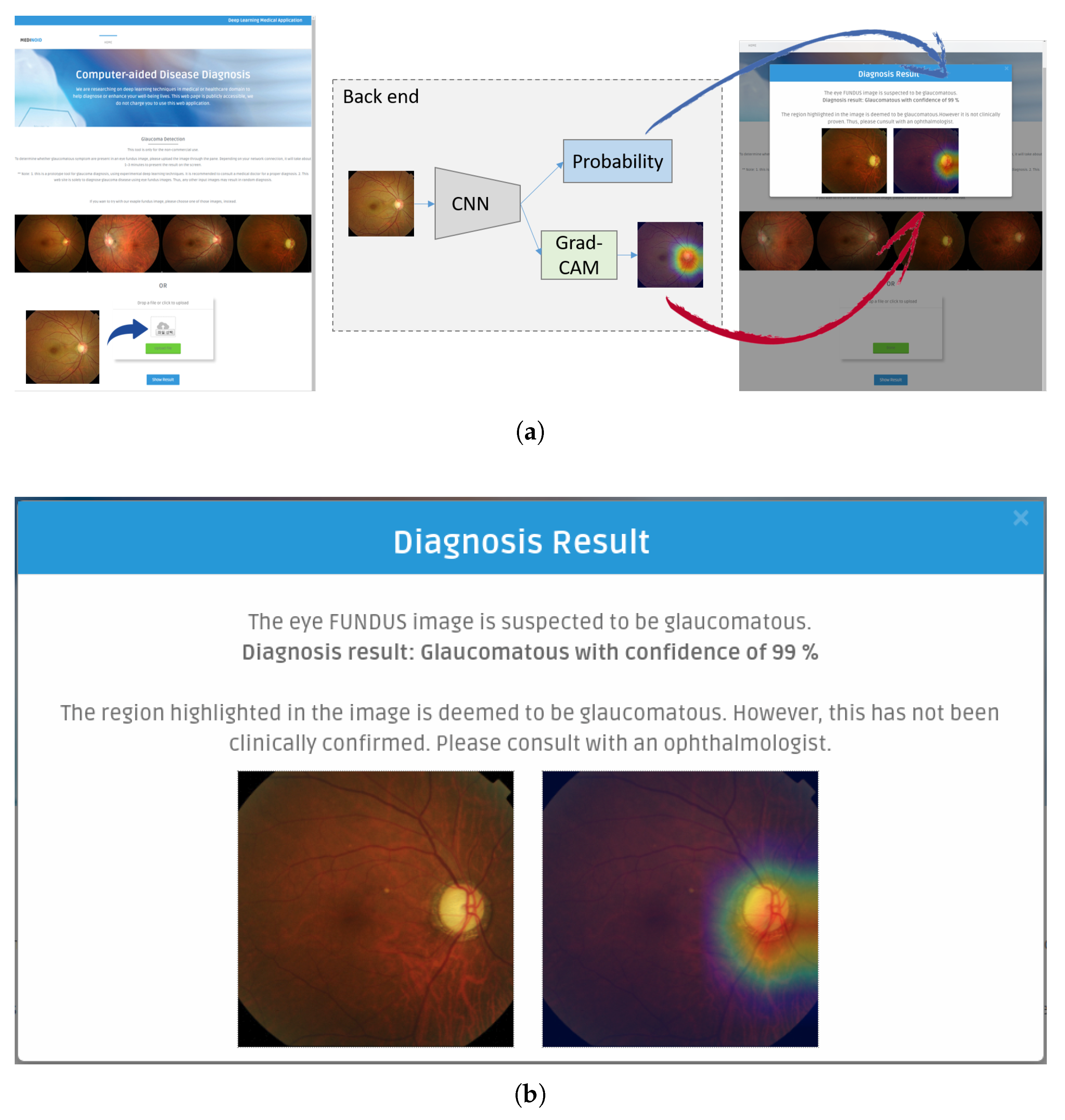
• Medinoid: We have developed Medinoid (http://www.medinoid.org), a publicly-available prototype web application for computer-aided diagnosis and localization of glaucoma in fundus images, integrating our predictive model. This web application is intuitive to use for medical doctors, as well as for people who have difficulties in accessing human experts and/or specialized medical imaging equipment.

Note that this paper is an extension of work previously presented at a conference [29], leveraging deeper models so as to be able to increase the effectiveness of diagnosis and additional datasets so as to be able to better evaluate generalization power. Furthermore, we present more in-depth experimental results and introduce Medinoid, a web application for both glaucoma diagnosis and localization.

The remainder of this paper is organized as follows. In Section 2, we provide an in-depth overview of our approach towards glaucoma diagnosis and localization. In Section 3, we outline our experimental setup, and in Section 4, we subsequently discuss the results obtained. Finally, we provide conclusions and directions for future research in Section 5.

2. Methodology

Our proposed approach encompasses two major computer vision tasks, namely image classification and localization. The first task outputs the diagnosis result (normal or glaucomatous) and the diagnostic confidence. Upon diagnosis of glaucoma, the second task outputs the most suspicious area in the given fundus image.

At the core of the classification task is a CNN architecture that acts as a feature extractor, returning a predicted output $y_i$ for the class i. The softmax function $\sigma =e^{y_i}/{\sum }_k{e}^{y_k}$ is then applied to calculate the probability of each class $k\in K$. We used the resulting probability of the predicted output as a measure of the diagnosis confidence, given that the softmax function normalizes the output into a distribution of K probabilities.

In our research, through a thorough comparison of various CNN architectures and datasets, we focused on obtaining a high diagnosis accuracy and a localization technique that is clinically meaningful. More details about the different CNN architectures used and the localization technique employed can be found below.

2.1. Convolutional Neural Networks

Given their high effectiveness, CNNs are currently the most widely-used technique in image classification [30,31,32]. Their strength stems from the use of convolutional filters that are composed of neurons, also known as receptive fields. Inspired by biological processes, the neurons convolve over local regions in the input layer and respond to certain patterns, as the visual cortex does to stimuli in a local space. This is an important characteristic because, unlike the full connectivity of ordinary neural networks, this local connectivity enables CNNs to handle high-dimensional inputs such as natural images by substantially reducing the number of parameters to compute. In addition, CNNs are able to learn and classify hierarchical features directly from raw input images (end-to-end learning), thus not needing extraction of hand-crafted features. As CNNs have been demonstrated to be highly effective across various general image classification tasks, including the ImageNet Large-Scale Visual Recognition Challenge (ILSVRC), which comes with more than 1.2 millions images distributed over 1000 classes [33], medical image analysis using CNNs followed quickly [34], targeting use cases such as diabetic retinopathy diagnosis [35] and chest pathology analysis [36,37].

To achieve our goal of effective glaucoma diagnosis, we explored three representative CNNs: (1) VGG Networks (VGGNets) [38], (2) Inception Networks (InceptionNets) [31], and (3) Residual Networks (ResNets) [39]. Compared with their predecessors such as LeNetand AlexNet, these networks are all based on deeper architectures, all achieving higher accuracies while maintaining lower error rates. A comparison of the accuracies achieved by the different types of networks can be found in

Table 2. Accuracies of different deep neural network models trained on the ImageNet Large-Scale Visual Recognition Challenge (ILSVRC)-2012-CLS. Top 1 accuracy: the class having the highest probability is the same as the true label. Top 5 accuracy: one class among the top 5 ranked classes (ranked according to decreasing probability) is the same as the true label [40].

Model	Top 1 Accuracy	Top 5 Accuracy
VGG-16	71.5	89.8
VGG-19	71.1	89.8
Inception-v4	80.2	95.2
Inception-ResNet-v2	80.4	95.3
ResNet-152	77.8	94.1

.

The aforementioned CNNs were able to obtain high levels of accuracy thanks to the availability of ImageNet. This implies that, to achieve similar levels of effectiveness for our use case of glaucoma diagnosis, we need a dataset of similar size to ImageNet or we need to modify the CNNs in question so that they are able to mitigate overfitting issues caused by the usage of a limited amount of data [34]. As such, starting from the CNNs in question, we incorporated several regularization techniques, including early stopping, data augmentation, dropout layers, and transfer learning [41], with the aim of achieving better model generalization.

In what follows, we explain the main characteristics of each model, with

Table 3. Overview of the different model configurations for VGG-16 [38], ResNet-152 [39], and Inception-v4 [31]. When the name of a model contains the label “B”, this means that the model adopted the settings from the paper that introduced the model in question. When the label “M” has been added to the name of a model, this means that our research context has been taken into account, resulting in the modification of settings, the addition of regularizers such as data augmentation and dropout, and/or a change of the optimizers used. RMSProp, Root Mean Squared Propagation.

Model	Input Size	Optimizer	Data Augmentation	# of Layers or Blocks
VGG-16-B	$224\times 224\times 3$	SGD	crop, horizontal flip	16 layers
VGG-16-M	$224\times 224\times 3$	ADAM	crop, horizontal flip, contrast adjustment	16 layers
ResNet-152-B	$224\times 224\times 3$	SGD	crop, horizontal flip	152 layers
ResNet-152-M	$299\times 299\times 3$	ADAM	crop, horizontal flip, contrast adjustment	152 layers
Inception-v4-B	$299\times 299\times 3$	RMSProp	crop, horizontal flip, brightness adjustment, contrast adjustment, hue adjustment, saturation adjustment	14 inception blocks
Inception-v4-M	$299\times 299\times 3$	RMSProp	crop, horizontal flip, contrast adjustment	14 inception blocks

summarizing the modifications we made.

VGGNets: Developed at and named after Oxford’s Visual Geometry Group (VGG), VGGNets [38] were the first models to combine small receptive fields with a size of $3\times 3$ with multiple CNN layers. VGGNets are constructed using several convolutional blocks that contain two to three convolutional layers, followed by a max pooling layer. VGG-16 is currently the most representative network, having a relatively low number of parameters, but a higher top 1 classification accuracy compared to VGG-19. Like ResNets, VGGNets require input images to be normalized, resulting in zero mean and unit variance. Furthermore, VGGNets and ResNets make use of the same input size.

VGG-16 in its original form uses Stochastic Gradient Descent (SGD) as an optimizer, also employing learning rate decay. In our research, however, we made use of the Adaptive Moment estimation (ADAM) optimizer [42], so as to be able to overcome a number of drawbacks of SGD, including a slow convergence and a high error fluctuation.

ResNets: Microsoft Research introduced ResNets in 2016 [39]. These models obtained the first place in the ImageNet and the COCO2015 competitions, covering the tasks of image classification, semantic segmentation, and object detection. The core idea behind ResNets is the use of a residual network, which leverages skip connections to jump over some layers, reducing the impact of vanishing gradients, as there are fewer layers through which to propagate. As such, the use of residual networks makes it possible to train networks that are deeper, obtaining lower training errors and higher levels of accuracy. Depending on the number of residual networks, ResNets come with certain variations. In our research, we used a ResNet with 152 layers (i.e., ResNet-152), given that this network, among the different ResNets available, is able to obtain some of the highest accuracy levels.

InceptionNets: Unlike VGGNets and ResNets, InceptionNets [31] make it possible to better focus on the location of features that are important for the purpose of classification. Since salient parts can have different sizes per image, choosing the right receptive field size is difficult. In addition, in deep networks, there is the issue of overfitting and the issue of vanishing gradients. Therefore, Google Research introduced a new module, called “inception”, having several receptive fields with a different size [43]. Specifically, filter sizes of $1\times 1$, $3\times 3$, and $5\times 5$ were used, making the network wider. After max pooling, each output is concatenated and then sent to the next inception module. Over the course of time, inception modules have been modified and improved, leading to more powerful InceptionNets. Inception-ResNet-v2 and Inception-v4 are currently the most effective networks. By default, InceptionNets take as input images with a size of $299\times 299\times 3$, with pixel values belonging to [−1, 1]. The optimizer used is also different from the previous networks: InceptionNets typically make use of the Root Mean Squared Propagation (RMSProp) optimizer [44].

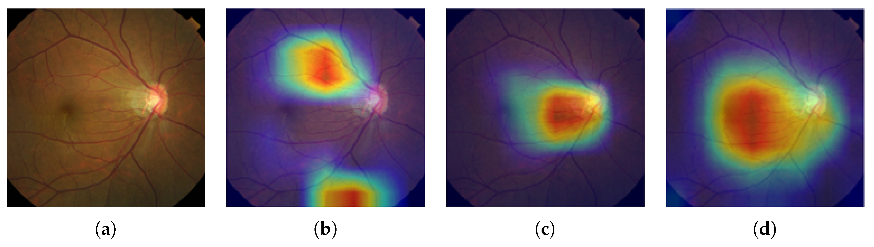
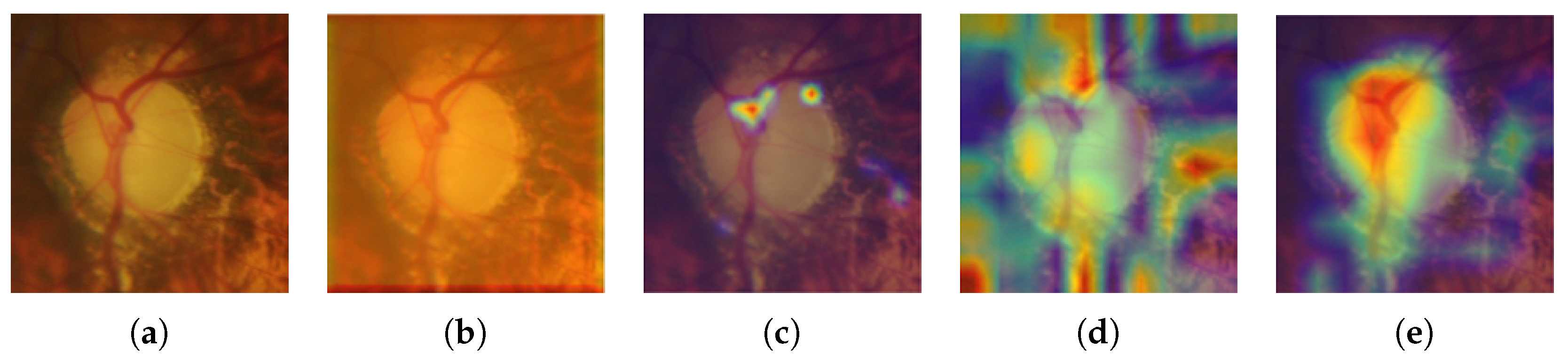
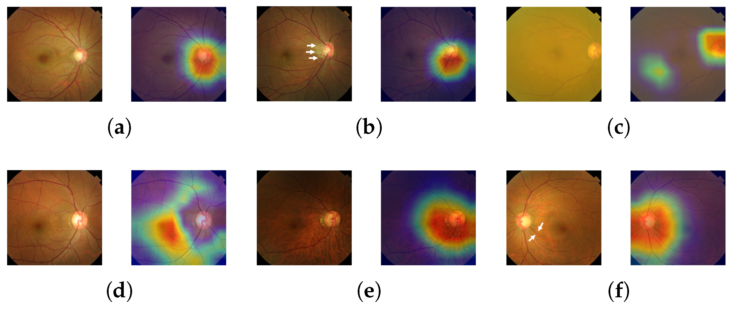
2.2. Grad-CAM

In practice, most medical images do not have any localization information, making it impossible to apply a state-of-the-art image segmentation approach like U-Net [30]. Therefore, we adopted Gradient-weighted Class Activation Mapping (Grad-CAM) [45] to localize glaucoma, a weakly-supervised learning approach, forgoing the need to give explicit segmentation information to a network. Grad-CAM generalizes the Class Activation Mapping (CAM) method originally proposed in [46], integrating gradient weights. CAM visualizes what CNNs look at when they classify the input, highlighting activations in the feature maps of the last convolutional layer, using the predicted output and backpropagation.

To produce the final localization map $L_{Grad-CAM}^g$ of the glaucomatous area, we first calculate the gradients of the predicted output $y^g$ for the class glaucoma with respect to the feature maps $A^k$ of the last convolutional layer, having width u and height v, where $k\in \{1,2,\cdots ,K\}$, and with K denoting the total number of feature maps. The result ${\displaystyle \frac{\partial y^g}{\partial A^k}}$ then goes through a global-average pooling process, calculating the weights ${\alpha }_k^g$ of the glaucoma class as follows:

$${\alpha }_k^g={\displaystyle \frac{1}{u\times v}}\sum _i\sum _j{\displaystyle \frac{\partial y^g}{\partial A^k}}.$$

(1)

Equation (1) can be interpreted as the importance of each feature map for the glaucomatous class. The weights and the corresponding feature maps are linearly combined and subsequently given as an input to a Rectified Linear Unit (ReLU) [47], with the latter only selecting the positive activations. The overall process can be formally summarized as follows:

$$L_{Grad-CAM}^g=\mathrm{ReLU}\left(\sum _k{\alpha }_k^g{A}^k\right).$$

(2)

3. Experimental Setup

3.1. Dataset: Fundus Images

Digital color fundus images (this study followed all guidelines for experimental investigation on human subjects, was approved by the Samsung Medical Center Institutional Review Board, and adhered to the tenets of the Declaration of Helsinki) were used from a database created by the glaucoma clinic of Samsung Medical Center in Seoul, Korea. All patients gave their informed consent to have their data used in our experiments. When the fundus images were taken, the camera had a magnification setting of 30${}^{\circ }$ or 35${}^{\circ }$. Moreover, the macula was center-positioned near the intersection of the crosshairs in the ocular. A fixation target was used to direct the gaze of the subject in the primary (straight ahead) position, so that the optic disc did not appear directly behind the lens. The color images were evaluated for quality by an experienced investigator. If the quality was not deemed adequate for assessment of the key features of the studied eye (such as optic disc morphology) and if no irremediable cause of inadequate quality was present (such as lens opacities or a pupil that did not dilate adequately), then the images were retaken.

The fundus dataset used for training contained 540 normal eye images and 1363 glaucomatous eye images, thus resulting in the use of a total of 1903 eye images. This dataset was randomly split into two sets, namely a training and a validation set, using a split ratio of approximately 4:1 (that is, the training dataset contained 1503 images and the validation dataset 400 images). The training set was used to fine-tune our models, whereas the validation set was employed to assess the generalization power of the models created during training. Apart from these two datasets, for testing purposes, 220 unseen fundus images were used: 55 normal eye images and 165 glaucomatous eye images. The images used came with different spatial resolutions, ranging from 1172–2500 pixels horizontally and from 1500–3200 pixels vertically.

Starting from the set of original fundus images, we created two derived datasets, as shown in Figure 2. For the first derived dataset, we center-cropped all images using a 1:1 ratio by cutting off unnecessary image areas (e.g., a black background sometimes containing image numbers and text). For the second derived dataset, we cropped the optical disc part from each image. The former set of images was named Dataset-C, and the latter set of images was named Dataset-OD. We created the two different datasets in order to be able to investigate the importance of the optic disc, given that most related work only made use of this part of the fundus images.

3.2. Implementation

Our approach towards glaucoma diagnosis and localization was implemented in Python 2.7, using Tensorflow 1.7, with all pre-trained models taken from Tensorflow Slim (https://github.com/tensorflow/models/tree/master/research/slim). Furthermore, our approach was run using two Intel(R) Xeon(R) E5-2620 2.4-GHz CPUs and an NVIDIA GeForce GTX TITAN X GPU.

We focused on regularizing and generalizing the different predictive models created by making use of different techniques, for instance mitigating overfitting and bias by adding a dropout layer as a regularizer at the end of each convolutional block, residual block, or inception block, depending on the type of model used. Our overall experimental setup can be found in Table 3.

Data pre-processing: In this phase, all the input images were re-sized and normalized before training, taking into account the pre-trained model settings [31,38,39]. For VGG-16-* and ResNet-152-B, we re-sized the input to $224\times 224\times 3$ and normalized the input using the following RGB means: R:105.51, G:54.52, and B:16.19 (as derived from the images in the training set). For ResNet-152-Mand Inception-v4-*, after re-sizing the input to $299\times 299\times 3$, we scaled the input values to the range [−1, 1] instead of [0, 255].

Data augmentation: Overfitting occurs frequently when combining a small-sized dataset with a deep neural network, as was the case for the given set of fundus images and the architectures used, with the latter coming with a large number of parameters that needed to be computed. In order to alleviate overfitting, we incorporated data augmentation, artificially amplifying the volume of data during training through image processing techniques (e.g., horizontal flipping, contrast adjustment, and brightness adjustment), and where these techniques are often used in the context of computer vision tasks. Based on a comparison of the accuracy of different data augmentation techniques in [48], we applied several random data augmentation methods, also taking into account the different models used (that is, for each model, we used different types of data augmentation).

Fine-tuning: When training from scratch, a model often initializes all parameters using random Gaussian distributions. This approach towards initialization is usually less accurate, with the model at hand needing more time to converge [34,49]. To avoid initialization issues, we employed models pre-trained on ImageNet, transferring their weights to our models, hereby also allowing for better generalization. Starting from these pre-trained weights, we fine-tuned all layers using the hyperparameter values shown in

Table 4. Hyperparameter values. We used early stopping to alleviate overfitting.

Model	Learning Rate	Number of Steps
VGG-16-B	0.00005	15,000
VGG-16-M	0.00005	15,000
ResNet-152-B	0.00001	8500
ResNet-152-M	0.00001	8400
Inception-v4-B	0.0005	15,000
Inception-v4-M	0.0005	15,000

, over Dataset-C and Dataset-OD. Note that the batch size used was 32.

3.3. Evaluation

Other than validation during the training phase, we implemented two more approaches to evaluate our model generalization. First, as explained in Section 3.1, we created a new dataset for testing purposes only. Second, we made use of RIM-ONEr3 [28], a publicly-available dataset of fundus images, to evaluate our model generalizability. Evaluation results obtained for both datasets are reported in the following section using several metrics: accuracy, recall (sensitivity), precision, F1 score, specificity, and Receiver Operating Characteristic-Area Under the Curve (ROC-AUC). These metrics were calculated as follows:

• Accuracy = ${\displaystyle \frac{\mathrm{tp}+\mathrm{tn}}{\mathrm{tp}+\mathrm{fp}+\mathrm{tn}+\mathrm{fn}}}$
• Recall (sensitivity) = ${\displaystyle \frac{\mathrm{tp}}{\mathrm{tp}+\mathrm{fn}}}$
• Precision = ${\displaystyle \frac{\mathrm{tp}}{\mathrm{tp}+\mathrm{fp}}}$
• F1 score = $2·{\displaystyle \frac{\mathrm{recall}·\mathrm{precision}}{\mathrm{recall}+\mathrm{precision}}}$
• Specificity = ${\displaystyle \frac{\mathrm{tn}}{\mathrm{tn}+\mathrm{fp}}}$

In the above, true positive (tp) denotes the number of glaucomatous images that have been classified as glaucomatous and true negative (tn) denotes the number of normal images that have been classified as normal. Similarly, false positive (fp) denotes the number of normal images that have been classified as glaucomatous, and false negative (fn) denotes the number of glaucomatous images that have been classified as normal. The first four metrics were used to evaluate the robustness of the deep learning models. The recall, specificity, and ROC-AUC were used to evaluate the models from a clinical point of view.

4. Experimental Results

Our experiments focused on evaluating both the model generalizability and the importance of the OD area in the fundus images. In this context, we first performed a quantitative analysis of the diagnosis accuracy, followed by a qualitative analysis of the effectiveness of localization.

4.1. Diagnosis Accuracy

To investigate the importance of the OD image area, the original dataset was used to create two new datasets, namely Dataset-C and Dataset-OD. The results, as obtained for the testing set and presented in

Table 5. Evaluation of model performance for glaucoma diagnosis over the testing dataset.

Data	Classifier	Accuracy	Recall	Precision	F1 Score	AUC Score
C	VGG-16-B	88%	88%	95%	91%	93%
	VGG-16-M	90%	88%	97%	92%	94%
	ResNet-152-B	88%	85%	99%	91%	94%
	ResNet-152-M	95%	95%	98%	96%	99%
	Inception-v4-B	90%	90%	96%	93%	97%
	Inception-v4-M	93%	92%	99%	95%	99%
OD	VGG-16-B	86%	95%	88%	91%	93%
	VGG-16-M	91%	90%	98%	94%	96%
	ResNet-152-B	87%	83%	100%	91%	95%
	ResNet-152-M	96%	95%	100%	97%	99%
	Inception-v4-B	91%	88%	99%	93%	97%
	Inception-v4-M	94%	92%	99%	95%	99%

and

Table 6. Clinical evaluation of model performance for glaucoma diagnosis over the testing dataset.

Dataset	Classifier	tn	fp	tp	fn	Sensitivity	Specificity
C	VGG-16-B	47	8	146	19	88%	85%
	VGG-16-M	51	4	146	19	88%	93%
	ResNet-152-B	53	2	141	24	85%	96%
	ResNet-152-M	52	3	157	8	95%	95%
	Inception-v4-B	49	6	148	17	90%	89%
	Inception-v4-M	54	1	151	14	92%	98%
OD	VGG-16-B	33	22	157	8	95%	60%
	VGG-16-M	52	3	148	17	90%	95%
	ResNet-152-B	55	0	137	28	83%	100%
	ResNet-152-M	55	0	157	8	95%	100%
	Inception-v4-B	53	2	146	19	88%	96%
	Inception-v4-M	54	1	152	13	92%	98%

, demonstrated that the models trained on Dataset-OD were more effective than the models trained on Dataset-C, in terms of all evaluation metrics used, thus confirming that the OD image area is a clinically-important region.

As shown by Table 5, and unlike the accuracy results obtained for the ImageNet classification task (see Table 2), the ResNet-152-M model was able to achieve the highest accuracy of 95% for Dataset-C and the highest accuracy of 96% for Dataset-OD. Compared to the images in ImageNet, the images in Dataset-C and Dataset-OD came with salient areas that had a relatively similar size and location. This homogeneity can for instance not be exploited well by InceptionNets, given the use of different convolutional filter sizes in each inception block, so as to be able to deal with salient areas that may differ from image to image in terms of size and location. Furthermore, when only considering the results presented for Dataset-OD in both Table 5 and Table 6, the ResNet-152-M model was able to outperform all other models, in terms of all metrics presented.

Table 6 additionally presents the sensitivity and the specificity of each model. For both metrics, the ResNet-152-M model, as trained on Dataset-OD, was able to obtain the highest values. This implies that the ResNet-152-M model was able to correctly screen both normal and glaucomatous eyes. This can also be qualitatively interpreted as follows: the ResNet-152-M model was able to provide more benefits at lower costs to patients. Furthermore, for both Dataset-C and Dataset-OD, the ResNet-152-M model obtained an AUC score of 99%, outperforming the other models (see Table 5 for the AUC score of each model).

To evaluate our model generalizability, we investigated two types of learning curves during training, making use of two representative models. Figure 3 illustrates the difference between the worst- and the best-performing models. In particular, Figure 3a,c illustrates the effectiveness of training and validation in terms of accuracy, showing that the accuracy increased for both VGG-16-B and ResNet-152-M as the number of steps increased. Contrarily, in terms of loss, Figure 3b,d shows that the VGG-16-B model did not optimize well at later steps, resulting in overfitting, while the ResNet-152-M model was able to converge well, resulting in good fitting.

Finally, we made use of RIM-ONE r3 [28], an external dataset, to provide a more in-depth evaluation of the generalization power of ResNet-152-M, our most effective model. The total number of fundus images in the RIM-ONE r3 dataset is 159, of which 85 eye images are normal and 74 eye images are glaucomatous. Although the characteristics (angle, eye range, camera model) of the fundus images are different from the fundus images collected at Samsung Medical Center, in general affecting the diagnosis accuracy of deep learning models, we applied our ResNet-152-M model, as trained on Dataset-C, to the RIM-ONE r3 dataset, given the visual resemblance between the two different datasets.

The authors of [17] performed experiments using five-fold cross-validation, with each validation set containing 17 normal and 14 glaucomatous eye images. For our external testing purposes, we split the RIM-ONE r3 dataset into five subsets, randomly selecting 31 images for each subset. The authors of [17] then evaluated the overall accuracy, sensitivity, and specificity. We implemented the same experiment, and the results obtained are summarized in

Table 7. Effectiveness of glaucoma diagnosis for RIM-ONEr3 [28]. Ours refers to the ResNet-152-M model. The ES model of [17] model used Entropy Sampling for feature extraction, whereas the CNN of [17] used a CNN. Both ES [17] and CNN [17] used a softmax classifier. The results were adopted from [17].

	Ours	ES [17]	CNN [17]	[50]	[51]	[24]
Accuracy	93.5	94.1	92.4	90.2	89.4	92.1
Sensitivity	92.9	92.3	90.1	87.4	86.4	89.8
Specificity	92.9	95.6	94.3	92.5	92.0	94.0

. Note that the models proposed in [17] may be biased towards the RIM-ONE r3 dataset (the authors of [17] did not provide testing results for a dataset different from the RIM-ONE r3 dataset). Moreover, as also mentioned in [17], the small size of the RIM-ONE r3 dataset made it challenging to apply CNNs, or even most other machine learning techniques.

4.2. Localization of Glaucomatous Areas

Unlike the evaluation of diagnosis accuracy, it is difficult to perform a quantitative evaluation of the effectiveness of localization, given that boundaries of optic disc notching or retinal nerve fiber layer defects cannot be clearly segmented in eye fundus images. In other words, there is no absolute gold standard available for a quantitative analysis of glaucomatous defect localization. Indeed, clinicians typically only confirm the presence of glaucoma by observing structural features [2,52,53]. Therefore, we made use of a qualitative approach towards evaluating the effectiveness of localization, asking clinicians for their informed opinion.

Figure 4 shows the localization results obtained by the *-M models for a fundus image taken from Dataset-C that was diagnosed as glaucomatous. For each model, the layer extracted for the purpose of localization was the last convolutional layer before the global max-pooling layer. Even though all classifiers correctly identified the given fundus image as glaucomatous, the location each network looked at was different, with the VGG-16-M model not succeeding in localizing the correct glaucomatous area in the given input image (as shown in Figure 4b). On the contrary, ResNet-152-M and Inception-v4-M were able to localize the glaucomatous area correctly. Given both Figure 4c and Figure 4d, the ResNet-152-M model produced a more precise localization than the Inception-v4-M model, with the produced localization also being more correct from a clinical point of view.

Figure 5 and Figure 6 visualize how models find the glaucomatous area per ResNet block in ResNet-152-M. Given both figures, we can again confirm that our model looked at the OD area to diagnose glaucoma. Having a look at the internals of ResNet-152-M, as illustrated in Figure 5, the leftmost image was the input image, and from the left to the right, we present the last convolutional layer of each residual block. As the input went from the lower layers to the higher layers, Figure 5 shows where the model looked at in order to make a classification decision, localizing where the glaucomatous region can be found in the heat map.

Both Figure 7 and Figure 8 show localization results obtained for our most effective model, namely ResNet-152-M, for fundus images taken from Dataset-C. In our test results, 209 images were correctly diagnosed and 11 images were wrongly diagnosed, given the human labels. Among the correctly-diagnosed images, the optic nerves in the true positives were all correctly localized, as shown in Figure 7a. For the true negatives, most of them were clinically well localized, as shown in Figure 7b. However, there were some atypical localizations, as indicated by the white arrows in Figure 7c.

Among the wrongly-classified images, there were three false positives and three false negatives. Regarding the false positives, each one of them was diagnosed wrongly for different reasons. In Figure 8a, we can observe the distribution of the normal retinal nerve fibers around each optic disc. In addition, we can observe a normal cup-to-disc ratio and a healthy RNFL in each fundus image. However, the model still showed glaucomatous features around the optic disc. Furthermore, the fundus image in Figure 8b shows a myopic tilted optic disc with large Parapapillary Atrophy (PPA) (white arrows). Though no RNFL defects were shown in the fundus image, the localized result clinically showed a positive diagnosis around the ONH and, in particular, in the inferior optic disc area. When investigating the last image in Figure 8c, we can observe that the image was not clear due to media opacity (as for instance caused by cataract). Therefore, even though the image looked normal, which meant that glaucoma was absent, the model diagnosed the image as glaucomatous.

The remaining erroneous results of the model stemmed from three false negatives. Given Figure 8, we can further analyze why the model was producing the aforementioned false negatives. The first example in Figure 8d was an interesting case because the human labeling was wrong and the model correctly diagnosed the disease. In other words, the image did not have any glaucomatous symptoms, which implied that it was a true negative. The second example in Figure 8e shows a myopic fundus image with a tigroid pattern in the overall retina. Clinically, it was difficult to detect whether RNFL defects were present in this type of retina. Only the cup-to-disc ratio can give information about the presence or absence of glaucoma. In this experiment, the model might have missed the glaucomatous cup-to-ratio morphology. The third image in Figure 8f seemed to point to early-stage glaucoma producing RNFL defects. Given that the RNFL defect width was relatively narrow, as indicated by the white arrows in the figure, it might not be detectable.

4.3. Medinoid

We integrated ResNet-152-M, our most effective model, into the back-end of Medinoid, a publicly-available web application for glaucoma diagnosis and localization. Medinoid takes as input a fundus image (JPG, PNG, or BMP), showing the diagnosis outcome to the user as soon as the given fundus image has been analyzed by the model in the back-end. If the input image has been diagnosed as normal, then the result window will show the decision made, as well as the diagnostic confidence. If the input image has been diagnosed as glaucomatous, then the result window will additionally show the localization of the glaucomatous area. An illustrative screenshot can be found in Figure 9.

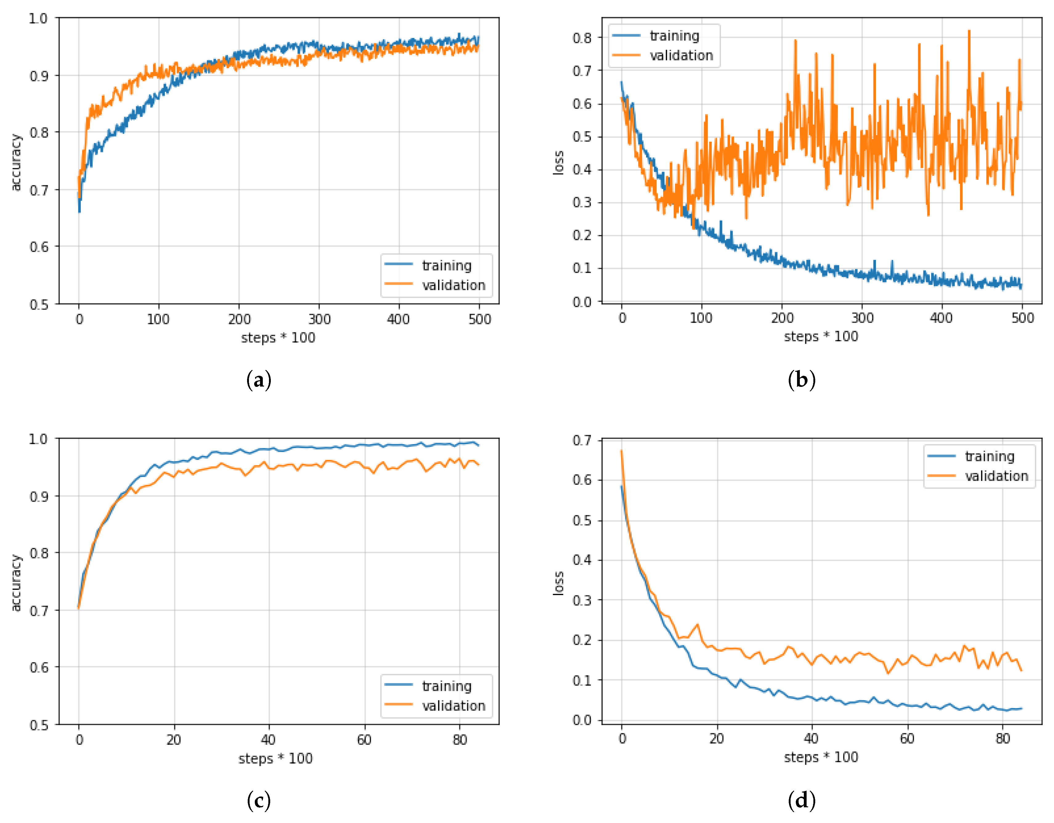
5. Conclusions and Future Research

In this paper, we introduced a new computer-aided approach towards glaucoma diagnosis and localization. The predictive CNN-based model we developed, namely ResNet-152-M, obtained the best diagnosis scores among all metrics used. Moreover, using Grad-CAM, a weakly-supervised localization method, our predictive model was able to highlight where a glaucomatous area can be found in a given input image. This demonstrates that the application of deep learning tools to medical images, even though the number of images available for training is typically small, can help doctors in diagnosing glaucoma in a more effective and efficient way. Lastly, we presented Medinoid, a web application that integrates our predictive model into its backend, making it for instance possible to diagnose glaucoma in a constrained medical environment.

If a set of training images is too small or if a set of training images is not representing well the general nature of the classes, then it is easy for a deep learning model to be biased towards the training set. In this context, we were for instance able to make the following observation: the experiments that made use of an external dataset produced lower accuracy scores than the experiments that made use of our own dataset. As a result, to mitigate model bias, future research will focus on incorporating various types of fundus images, for instance taken by other medical equipment using different angles, so as to be able to include more diversity. Furthermore, in future research, we plan to leverage our experience with deep learning-based diagnosis and localization of glaucoma in the context of other diseases, particularly paying attention to disease diagnosis and localization using 3D medical imagery.